Anomalous upper mantle beneath the Central Andes : isostasy and Andean uplift
12
0
0
Texto completo
(2) 2. INTROCASO - Anomalous upper mantle (Andes). INTRODUCTION It has been pointed out that beneath the Central Andes, there could be: (1) cooling produced by the Nazca Plate subduction beneath the continental lithosphere (Grow and Bowin 1975; Introcaso and Pacino 1988) and (2) significant heating on the lithospheric mantle (Froideveaux and Isacks 1984; Introcaso and Pacino 1988; Isacks 1988). Here, we have analyzed the (1) and (2) density anomaly effects either on the gravity or on the Andean uplift. From (1), there would be high gravity and subsidence eci, whereas from (2) there would be gravity diminution and elevation eei. Let us consider mechanism (1). The subducted plate may produce subsidence due to the following two facts: (a) the oceanic plate mean temperature is about 350°C (0°C on the top and 700°C on the bottom). When subduction takes place, the plate is located at the hot mantle, lower than 70 or 80 km deep. Temperatures there reach 1 200°C at depths of 140 km. Thus, a relative cooling is produced; (b) moreover, petrologic phase changes are probable, at adequate pressure and temperature. So, oceanic crust may become eclogite (density of about 3.5-3.6 g×cm-3) or gardnet-peridotite (» 3.38 g×cm-3). Both circumstances produce contraction, subsiding the column that contains the subducted plate masses anomalies. According to Grow and Bowin (1975) and Dorman and Lewis (1972), the anomalous effects have been considered for isostatic evaluation until 300 km and 400 km respectively. For better understanding, let us think that the relative cooling mentioned in (a) results in a density increase of +0.03 g×cm-3 for the mantle normal density (estimated to be 3.3 g×cm-3). If the length of a vertical column that intersects the subducted oceanic lithosphere were 80 km, the contraction ec would be 80×(1 - 3.30/3.33) = 0.72 km. Under such conditions, if a phase change on the oceanic crust 7 km thick took place, basalt with a density of 2.9 g×cm-3 would become, for example, eclogite with a density of 3.5 g×cm-3, producing a subsidence of 7×(0.6/3.50) = 1.2 km by contraction. Let us return to point (2). It is well known that the large magmatic activity consistent with the highest elevation below the Central Andes strongly supports the existence of a thermal root (Froideveaux and Isacks 1984) although a thermal anomaly can justify only part of a great mountain's elevation (Froideveaux and Ricard 1987). So we need at least one additional method. In order to explain part of the Central Andean uplift, we assume lithospherical heating from the large recognized Quaternary volcanism, associated with subduction (Froideveaux and Isacks 1984; Introcaso and Pacino 1988; Introcaso 1991). Moreover, Isacks' data (1988) obtained from 22 transversal Andean sections, topography was assumed by the mentioned author as the result of a combination of crustal shortening and lithospherical heating due to a thermal anomaly, agreeing with the Quaternary volcanic arc located over 27°S latitude. For better understanding, let us consider a thermal anomaly with DT = 300°C located on the lower half of the thermal lithosphere, 140 km thick. To keep the isostatic equilibrium of the column, the expansion will produce an. elevation V = (0.03/3.27)×70 km = 0.64 km. In this expression we assume lithospherical density as 3.3 g×cm-3, diminishing to 3.27 g×cm-3 = (3.30 - 0.03) g×cm-3 when heating is present. In order to analyze the heating below the Central Andes, Introcaso and Pacino (1992) prepared an isostatic correction chart, under the thermal hypothesis, or Pratt's hypothesis. The chart, with maximum corrections of +60 mGals, was prepared assuming a thermal expansion coefficient a = 3×10⁻⁵/°C. Using this chart, the corrections can be carried out in a few minutes. In this paper we analyze four theoretical models inspired on the Central Andes. They are all isostatically compensated and their main features are the following: (a) Classical crustal model (or Airy model); (b) model with crustal heterogeneities (Andean masses and crustal root) and subcrustal heterogeneities (lithospherical thermal root); (c) model that combines crustal thickening with thermal contraction effect due to the subducted plate; (d) model which combines all the anomalous effects mentioned before. From them, we demonstrate that:. "belowThethemodel adopted for evaluating isostatic equilibrium Central Andes is not critical. "crustalBouguer anomalies are principally controlled by roots beneath the Andes. If we admit a less. significant incidence of the magmatic addition mechanism, the chief mechanism for explaining the Andean uplift is the crustal shortening.. "mantle, If there exist anomalous thermal effects on the upper they could produce variations of less than 10% (5 to 6 km) on the crustal roots; changes of 16% (thermal expansion) and +18% (thermal contraction) on the crustal shortenings respect to the classic Airy model.. "24.5°SFinally, two Andean gravity models located at 22°S and latitude with peak Bouguer anomalies of 400 mGals, can be explained better by a model like model 2 (for example, it is consistent with seismic data at 24.5°S latitude). Yet inadequate changes in the initial conditions: normal crustal thickness, difference of density between lower crust and upper mantle, etc. allow us to show that other alternative models can also work, for example model 1. HETEROGENEITIES ON THE UPPER MANTLE THEORETICAL MODELS As we have just pointed out, there would exist anomalous effects below the Central Andes, produced by heating on the lower part of the crustal lithosphere, and by cooling due to the cold subduction of the Nazca Plate. For better analyzing these effects, we have prepared four theoretical models accurately isostatically compensated at different levels. These models are preliminary models, in the sense that they only admit density variations with temperature changes. Relationships between temperature and mantle viscosity, changes in lithosphere-astenosphere density and changes in the pressure gradient, have not been taken into account. All models assume isostatic compensation, and since the Andean excedent cannot be modified, the.
(3) 3. Boletín del Instituto de Fisiografía y Geología 71(1-2), 2001.. redistribution of the masses which tend to keep the equilibrium demands the crustal root to be thickened respect to the Airy model, in -20% to +20%. Our models show the following characteristics (Fig. 1): - Model 1 (for Airy model) (Fig. 1A): Andean masses, ma (ABCDA), width: 350 km; density st = 2.67 g×cm-3; maximum altitude ht = 4 km; topographic section area: 1270 km2, normal crustal density (below the sea level) sc = 2.90 g×cm-3; normal crustal thickness Tn = 35 km; upper mantle normal density sm = 3.30 g×cm-3; root that compensates the topographic excess DR1 = 26.7 km, where st x ht = 6.675 x ht (1) DR1 = sm - sc with differential density sm - sc = 0.4 g×cm-3 = (2.90 - 3.30). Isostatic compensation takes place at a depth of 300 km, and crustal thickness would be defined from R2i and R3i by: æH st H ö Ds DR4i = hti + ç ''C - 'T ÷ ´ ´s m (4) sm -sc è sm sm ø sm -sc if: Ds = sm - s'm = s''m - sm . Shortening in model (4) is 288 km. Fig. 2 shows the differences among the root thicknesses of the different models. The maximum root thickness in model 1 (Fig. 2A) is 26.7 km. In model 2 (Fig. 2B), it is reduced to 21.4 km at great part of the root. In model 3 (Fig. 2C), on the contrary, it increases reaching 32.7 km. As we can see in Fig. 2D, differences of about 11 km between models 2 and 3 show that the probable upper mantle heterogeneities may produce significant changes in crustal thickness, since the isostatic equilibrium must be kept without modifying the exposed distribution of the Andean masses.. g×cm-3. The shortening in this model is 278 km, as we will see when addressing the subject more specifically.. BOUGUER ANOMALIES AND ISOSTATIC ANOMALIES ORIGINATED BY THE MODELS. - Model 2 (Fig. 1B): The Andean masses ma are now perfectly balanced by a combination of a crustal root (26.7 5.3) km = 21.4 km thick at the central zone, and a thermal root EFGHE located at the lower half of the thermal lithosphere 140 km thick, where pressures are equal. Differential density s'm - sm = -0.03 g×cm-3, i.e., with s'm =. Fig. 3A shows the Bouguer anomalies (effects from all the anomalous masses located below the sea level) produced by the four described models. They present approximately the same wavelengths and maximum differences (model 3 model 2) of 42 mGal, i.e., 11% respect to the mean Bouguer anomaly. These results anticipate the idea that the model chosen to evaluate the isostatic equilibrium is not critical. In fact, Fig. 3B shows the isostatic anomalies corresponding to models 2, 3 and 4 obtained after performing the isostatic corrections obtained from the Airy model's crustal root gravimetric effects with opposite sign. The isostatic anomalies present a clear decreasing respect to the great Bouguer anomalies (about 10%). This decreasing points out:. 3.27 g×cm-3, assuming a thermal expansion coefficient a = 3×10⁻⁵/°C. The isostatic compensation in this model takes place at the bottom of the thermal lithosphere, that is at a depth of 140 km. Shortening in this model is 230 km. The equation for defining the crustal root is: st s m - s m' s m D R = ´ h H ´ 2i ti T (2) sm -sc s m - s c s m' where HT is the lithospherical column piece thickness before heating. After heating, the thickness will be HTi = HT ×s m/s'm . Partial melt may take place from an abnormally heated zone. Since that, magmatic addition in the crust is probable. We will see this when focusing on shortenings. - Model 3 (Fig. 1C): Isostatic balance of the Andean masses ma takes place at a depth of 300 km, where pressures balance. It involves a crustal root with maximum thickness R3i = (26.7 + 6.0) km = 32.7 km combined with an effect produced by the cold subduction (IJKLI) of the plate dipping a = 30° between 100 km and 300 km; we have assumed a density contrast of +0.03 g×cm-3 = s''m - sm, where s''m is the anomalous density = 3.33 g×cm-3. Crustal root R3i is here defined by st s '' - s m s m DR3i = hti + H C m ´ (3) sm -sc s m - s c s m'' where HC is the subducted Nazca Plate vertical column thickness before contraction. After contraction, thickness will be HCi = HC×sm/s''m. Shortening in this model is 338 km. - Model 4 (Fig. 1D): It involves crustal thickening, thermal expansion and contraction produced by the Nazca Plate.. " ". an isostatic equilibrium tendency in all the models, and that the model chosen to evaluate isostatic equilibrium is not critical. SHORTENING BACKGROUNDS. Shortening is no doubt present in the Andean elevation, as it is confirmed by the following values: 115 km in Central Perú (Megard 1978); 190 km in the Peruvian Andes (Suarez et al. 1983); 150 km to 225 km at 18°S latitude (Sheffels et al. 1986); 185 km for the Andean latitudes 21°S-22°S (Giesse and Reutter 1987); 250 km at 22°S combined with heating (Isacks 1988). In Andean sections located at 30°S, 32°S (and 33°S) and 35°S, Introcaso et al. (1992) report shortenings of 150 km, 130 km and 90 km respectively. Based on the areas of 22 sections of the Andean excedents (in km2), Isacks (1988) found a gap on the seismic attenuation (Q) transversal section between 27°S and 15°S latitudes, respect to the values located between 35°S and 27°S latitudes that in his graph (fig. 6 in his paper) follow a regular sequence. He attributed this excess to heating at the lower half of the thermal lithosphere 140 km thick. Discounting this effect, the maximum shortening diminishes from about 320 km to 250 km in the South American elbow. His model does not involve magmatic.
(4) 4. INTROCASO - Anomalous upper mantle (Andes). 0. 100. 200. 0. B A. 300. 400. 500. C. 600. 700. D. 800. km. km. 2.9g/cm3 -0.4g/cm3. DRt. 3.3g/cm3. -100. MODEL 1. -200. A. Sh= 278 km. -300. 0. 100. 200. 0. B A. 300. 400. 500. C. 600. 700. D. 800. km. 3. km. 2.9g/cm 3. DRt. -0.4g/cm. 3.3g/cm3 F. E -100. -0.03g/cm3. Eh + L/2. H. G. MODEL 2. -200. B Sh= 230 km. -300. 0. 100. 200. 0. B A. 300. 400. 500. C. 600. 700. D. 800. km. 3. km. 2.9g/cm -0.4g/cm3 I. -100. DRt. J. +0.03. -0.03g/cm3 H. MODEL 3. -200. 3.3g/cm3. 80.83 - Ec. Sh= 338 km. -300. 0. 100. 200. 0. B A. L. 300. 400. 500. C. K. C. 600. 700. D. 800. km. 3. km. 2.9g/cm -0.4g/cm3. DRt. 3.3g/cm3 F. E -100. I. J. +0.03. -200. -300. MODEL 4. -0.03g/cm3. Eh + L/2. H. G. 80.83 - Ec. Sh= 288 km. L. K. D. Figure 1. Theoretical models that explain the Central Andean uplift (ABCD). A: Model 1 or Airy Model; B: Model 2 that compensates the Andean masses by means of a combination of a crustal root (DRt) and a lithospherical thermal root (EFGH); C: Model 3 that compensates the Andean masses by means of a combination of a crustal root and the Nazca Plate cold subduction effect (IJKL); D: Model 4 that compensates the Andean masses by means of a combination of a crustal root and the upper mantle heterogenities effects (Models 2 and 3). Figura 1. Modelos teóricos que explican el levantamiento andino (ABCD). A: Modelo 1 o Modelo de Airy; B: Modelo 2 que compensa las masas andinas por medio de la combinación de una raíz cortical (DRt) y una raíz térmica litosférica (EFGH); C: Modelo 3 que compensa las masas andinas por medio de la combinación de una raíz cortical y el efecto frío de la subducción de la Placa de Nazca (IJKL); D: Modelo 4 que compensa las masas andinas por medio de la combinación de una raíz cortical y los efectos de las heterogeneidades del manto superior (Modelos 2 y 3)..
(5) 5. Boletín del Instituto de Fisiografía y Geología 71(1-2), 2001.. km. km. A. km. km. B. km. km. C. km. km. D. Figure 2. Crustal thicknesses of models 1, 2, 3 and 4 (see Fig. 1) to keep the Andean masses isostatic equilibrium. A: crustal thickness (61.7 km) corresponding to model 1 (Fig.1A); B: diminished crustal thickness (maximun values: 60.9 km and 56.4 km) corresponding to model 2 (Fig. 1B); C: increased crustal thickness (maximun values 67.7 km and 66.2 km) corresponding to model 3 (Fig. 1C); D: difference between the crustal thickness corresponding to models 3 and 2 (maximun: 11 km). Figura 2. Modelos 1, 2, 3 y 4 de espesores corticales andinos (véase Fig. 1) manteniendo el equilibrio isostático de las masas andinas. A: espesor cortical (61.7 km) correspondiente al modelo 1 (Fig.1A); B: espesor cortical disminuído (valores máximos: 60.9 km y 56.4 km) correspondiente al modelo 2 (Fig. 1B); C: espesor cortical incrementado (valores máximos: 67.7 km y 66.2 km) correspondiente al modelo 3 (Fig. 1C); D: diferencia entre el espesor correspondiente a los modelos 3 y 2 (máximo: 11 km)..
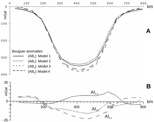
(6) 6. INTROCASO - Anomalous upper mantle (Andes). 0. 100. 200. 300. 400. 500. 600. 700. 800. km. mGal. 0. -100. A -200. -300. -400. Bouguer anomalies (AB1): Model 1 (AB2): Model 2 (AB3): Model 3 (AB4): Model 4. 35 mGal. B AI2,1. 0. km 200. 400. -35. AI3,1. 600. 800. AI4,1. Figure 3. A: Bouguer anomalies of Models 1, 2, 3 and 4 (see Fig. 1). They present the same wavelengths but little differences in amplitude: maximun 11% between Models 3 and 2 (Fig. 1C and 1B); B: Isostatic anomalies AI2,1, AI3,1 and AI4,1 of Models 2, 3 and 4 (Fig. 1 B-D) calculated from the classic Airy Model (Fig. 1A). They differ very little between them (maximun difference of less than 10%) pointing out the existence of isostatic equilibrium. Figura 3. A: Anomalías de Bouguer de los Modelos 1, 2, 3 y 4 (véase Fig. 1). Estos presentan las mismas longitudes de onda pero ligeras diferencias en amplitud: máximo 11% entre los Modelos 3 y 2 (Fig. 1C y 1B); B: Anomalías isostáticas AI2,1, AI3,1 y AI4,1 de los Modelos 2, 3 y 4 (Fig. 1 B-D) calculadas a partir del Modelo de Airy clásico (Fig. 1A). Estas difieren muy poco entre sí (máxima diferencia por debajo del 10%) resaltando la existencia de equilibrio isostático.. addition. We have considered Isacks' proposal (1988) in the analysis of our models on 22°S and 24.5°S, finding that Isacks' lithospheric and gravimetrical results will be consistent if the crustal model presents a crustal density excess of 1.3% at 22°S, respect to the averaged density of all the crust, and of 2.7% at the lower crust (root) respect to the model located at 24.5°S. Let us now return to our theoretical models. Model 1 gives a shortening of Sh = (At+AR)/Tn = 278 km; where At is the transversal area of the topographic excedent (in km2); AR is the compensating root (= 6.675×At, Introcaso et al. 1992) and Tn is the initial crustal thickness (= 35 km). Since At = 1270 km2, At+AR = 7.675×At. If we admit that the crustal thickening can be due, in part, to magmatic addition, there will be less necessary shortenings. In fact, Kono et al. (1989) considered that the material incorporated to the crust in the Peruvian Andes would be 15% of the anomalous heated zone of about 30 000 km2. So, for our model 2, the crust would incorporate approximately 4 500 km2 of materials of the upper mantle (since the anomalous heated zone is 23 450 km2), and it would suffer a thickening of (3 518 / 335) km » 10.5 km for our theoretical models. For this shortening, and assuming a constant crustal density, the isostatic equilibrium requires an elevation of (10.5 / 7.675) km = 1.368 km. So, the whole crustal thickening (10.5 km) is distributed between 1.368 km (topographic uplift) and 9.132 km (root). Rigorously, Isacks (1988) considered that. magmatic addition is not significant, and Ramos (pers. comm. 1992) estimates that it could be only 5%, so that the average thickening added would be only 3.5 km, contributing to the Andean elevation in only (3.5 / 7.675) km = 0.456 km. Considering the four theoretical models, with and without magmatic addition, we will have the shortening values of Table 1. Both the root area variations AR (column 3) and the coefficients AR/At (column 4) anticipate the shortening Sh changes (columns 5 and 6). Finally, magmatic addition justifies part of the crustal thickening and diminishes the shortenings (column7). In what we have seen we have assumed simplifying the problem- that the intrusion used to keep the same density as the medium crustal density . If we consider intrusions whose densities are different to (for example acid or basic intrusions) medium crustal density will change, since as we have seen, the intruded volume is not considered as very significant. Assuming changes in the density, it is easy to demonstrate that the relationship sc DR i = hi s m - sc. changes, although only a little. MODEL BACKGROUNDS Schmitz et al. (1993) presented a seismic model on 24.5°S latitude, with a maximum Moho depth of 60 km. High and.
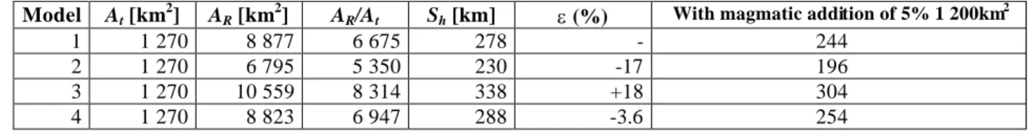
(7) 7. Boletín del Instituto de Fisiografía y Geología 71(1-2), 2001.. Table 1. Column 1: Models 1, 2, 3 and 4 (Fig. 1); column 2: Area At of the Andean excedent; column 3: areas AR of the roots; column 4: relationship AR/At; column 5: shortenings Sh; column 6: Model 1 shortening porcentual variations respect to Sh. Tabla 1. Columna 1: Modelos 1, 2, 3 y 4 (Fig. 1); columna 2: Area At del excedente andino; columna 3: áreas A R de las raíces; columna 4: relación AR/At; columna 5: acortamientos Sh; columna 6: variaciones de acortamiento porcentual del Modelo 1 respecto a Sh.. Model 1 2 3 4. At [km2] AR [km2] 1 270 8 877 1 270 6 795 1 270 10 559 1 270 8 823. AR/At 6 675 5 350 8 314 6 947. Sh [km] 278 230 338 288. low velocity changes in lower crust are significant in this model. Northward this section, on 21°S, Schmitz (1993) and Wigger et al. (1993) found a maximum Moho depth of about 65 km. On 22°10'S between 67.7°W and 71.5°W longitudes (Porth et al. 1990) they have also found low and high velocities, whose average in the lower crust is 6.2 km/s. This zone continues downwards until at least 65 km. They have found the following sequence of velocities and densities in the continental area: 22°10'S (only from Chile to the occidental Cordillera) -Crust 6 to 6.2 km×s-1 (upper crust) 2.78 g×cm-3 6.2 km×s-1 (lower crust) 2.90 g×cm-3 -1 6.7 to 7.4 km×s (intermediate crust) 2.90 to 3.10 g×cm-3 -Upper mantle 8.2 km×s-1 3.25 g×cm-3 24.5°S -Crust 6 to 6.2 km×s-1 (upper crust) 2.66 to 2.75 g×cm-3 6 to 6.6 km×s-1 (lower crust) 2.90 g×cm-3 -1 6.7 to 7.2 km×s (intermediate crust) 2.94 g×cm-3 -Upper mantle 8.1 km×s-1 3.26 to 3.28 g×cm-3 Density contrasts between lower crust and upper mantle are from 0.35 g×cm-3 to 0.38 g×cm-3. 22°S and 24.5°S latitudes sections, compiled by Porth et al. (1990) present as a capital fact, low velocities of 6 km×s-1, 6.2 km×s-1 and 6.6 km×s-1 in lower crust. According to the expression of Birch (1961): s=. VP + 2.55 3.31. and with Woollard (1959) relationships, a velocity decreasing of 0.1 km×s-1 would produce a density decreasing of 0.03 g×cm-3. At this point, we must take into account that these direct relationships not always hold. In fact, Woollard (1970) pointed out that the amount of Fe/Mg will play a decisive role, since a decreasing in the amount of Fe would produce a decreasing in density, while velocity VP would increase. Moreover, it is useful to point out that Araneda et. With magmatic addition of 5% 1 200km2. e (%) -17 +18 -3.6. 244 196 304 254. al. (1985) have found high conductivity with high gravity in the zone that we are analyzing, between 68°W and 69°W. Speculatively, they explain this by basic material intrusion (high density with high gravity) and high conductivity by strong mineralization near the intrusive margin. Another alternative proposed by the mentioned authors is that there would exist two consecutive intrusions. A first one, more basic, that would affect gravity, and a second one younger and acid, over the basic complex that would have affected conductivity. As we have seen, the value adopted by the German workers for the lower crust density is 2.90 g×cm-3. This value agrees with the one adopted by Introcaso and Pacino (1988) and Introcaso et al. (1990). These authors have considered a value of 3.30 g×cm-3 for the upper mantle density. Fortunately, the gravity models mainly depend on the difference of density between crust and upper mantle. So, Haak and Giesse (1986) pointed out that the Bouguer anomaly maximum amplitude of 400 mGal below the central Andes, may be wholly justified by means of the lower crust-upper mantle differential density without the necessity of other contributions, as for instance the intermediate or upper crust contributions. At the same time, these models allow us to explore different alternatives. The choice of one or another depends -as we will see- on the crustal thickness obtained from the seismic method. Our gravimetric models correspond to 22°S and 24.5°S sections (see location in Fig. 4). The gravimetric values of both sections were obtained from Abriata and Introcaso (1990) and Introcaso and Pacino (1988). Let us see the main characteristics of these profiles. Gravity Section on 22° South Latitude (Fig. 4a) The section is located near 22°S latitude (see Fig. 4a). It extends westwards from 62°W meridian, crossing Tarija city (Ta), Tupiza city (Tu) and San Pablo city (SP) until the International boundary with Chile, where it continues passing Chuquicamata and reaching the Coast at Tocopilla city (To), penetrating into the Pacific Ocean until 73°W longitude. The whole extension of the itinerary is approximately 1 200 km, involving: a) Pacific ocean sector 300 km b) Chilean continental sector 200 km c) Bolivian oceanic sector 700 km The profile crosses: (1) Coast Cordillera; (2) Central Valley (Chilean Precordillera); (3) Andes Cordillera or Principal Cordillera; (4) Altiplano-Puna; (5) Oriental Cordillera; (6) Subandean Ranges; (7) Chaco-.
(8) 8. INTROCASO - Anomalous upper mantle (Andes). shows the isostatic anomalies in the continental sector and the free air anomalies -as usually- in the sea. We must note that the gravimetric section in Fig. 5A presents two significant exceptions: (1) under the Chile trench zone, where they are strongly negative (» -100mGal) as it was previously recognized by Introcaso and Pacino (1988) and (2) in the Oriental Cordillera zone, where it is significantly positive (+80mGal). A similar case was found by Kono et al. (1989) for the Peruvian Andes section (Nazca-Punta Maldonado). They have pointed out decompensation in the Eastern Cordillera, and compensation in the Western Cordillera. Here, it would exist a lack of crustal root, estimated in 5 to 10 km (Abriata and Introcaso, 1990). Giesse and Reuter (1987) have admitted crustal delamination originated by an ascending heating counterflow caused by the oceanic plate subduction.. Figure 4. Andean gravimetric sections itinerary, located at 22°S (a) and 24.5°S (b) latitudes. Figura 4. Secciones gravimétricas andinas localizadas en latitudes 22°S (a) y 24.5°S (b).. Pampean flatness. Free air and Bouguer anomalies in Bolivia were taken from the Bolivian gravity charts presented by Tellería (1992). Bouguer anomalies are simple, without topographic corrections. Because of this, models are preliminary. Altitudes arise from satellite-measured computer files, given by Argentine Antarctic Institute. At the Chilean continental sector, Götze et al. (1987) and Draguicevic (1970) values were taken. In the Pacific Ocean sector, bathimetry and Free Air anomalies values were taken from Bowin et al. (1981), Hayes (1966), and Fisher and Raitt (1962). In these sections we detach the following values: Oceanic Sector: maximum depth of the Chile trench, 7 430 m; maximum free air anomaly under the trench, -228 mGal. Free Air anomalies were changed into Bouguer anomalies, replacing the sea water by continental masses, as we have just done on other sections (Introcaso et al. 1992). Continental (Andean) Sector: maximum altitude of measure, 4 669 m; maximum Bouguer anomaly, -414 mGal; maximum free air anomalies, +100 mGal at the Central Andes and +150 mGal near the Oriental Cordillera. Isostatic compensation was analyzed using an Airy model as model 1 (Figs. 1A and 2A). From the compensating masses or crustal roots obtained with DR = 6675×ht where ht is the topographic altitude. As it was demonstrated by Introcaso (1993) and here (Fig. 3B) the selected model is not critical to evaluate the isostatic equilibrium. Once Bouguer anomalies are corrected by gravimetric effects that compensating masses originate the resulting isostatic anomalies are small enough. Fig. 5A. Gravity Section on 24.5°S (Fig. 4b) This section also extends in EW direction, about 300 km inside the sea, from the Chilean coast passing Socompa and going on with a small dip towards S-SE through the same geological provinces from W to E, until reaching after crossing Santa Bárbara range (Fig. 4b) the foreland sector. Gravity, altitudes and marine depths values were obtained from the following sources: for the oceanic sector Hayes (1966), Fisher and Raitt (1962); for the continental sector in Chile Wuenschell (1955), Götze et al. (1990). The satellite-measured elevation computer files given by the Argentine Antarctic Institute were also used. The most significant results are: In the oceanic sector: maximum trench depth 8 200 m; maximum free air anomaly under the trench -252 mGal. As in the former cases, Bouguer anomalies were also calculated in the sea. In the continental sector: maximum Bouguer anomaly below the Andean axis -400 mGal; maximum altitude of measuring 3 889 m (Cerrato 1975). The isostatic equilibrium evaluation in the oceanic zone also shows a remarkable negative free air anomaly, as in the 22°S. As it is well known, in both cases the trench region is decompensated in isostasy usual terms. In the continental zone, the isostatic anomalies are small, pointing out that -in general terms- the equilibrium predominates (Fig. 5B). For both models, we have begun inverting the regionalized Bouguer anomalies with the following initial conditions:. ". "Normal" crust thickness Tn = 35 km, agreeing with the values adopted by Kono et al. (1989) and Giesse and Reuter (1987).. ". Differential density lower crust-upper mantle -0.40 g×cm-3, according to Introcaso et al. (1992), and less than 5% with the values adopted by Grow and Bowin (1975), Woollard (1969) and Draguicevic (1970). In order to separate the regional values, the observed Bouguer anomalies were processed by the filter method proposed by Pacino and Introcaso (1987). The method is based on upward continuation and inversion. Inversions were performed using Talwani et al. (1959) method, optimized by Marquardt (1963) algorithm. An analogous procedure was followed and commented when.
(9) 9. 150 100. mGal. Boletín del Instituto de Fisiografía y Geología 71(1-2), 2001.. Coast. 50. km. 0 200. 400. 600. 800. 1000. A. 1200. -50 -100. 150 100. mGal. Isostatic Anomaly Free Air Anomaly. Coast. 50. km. 0 200. 400. 600. 800. 1000. B. 1200. -50 -100. Isostatic Anomaly Free Air Anomaly. Figure 5. Isostatic and Free Air anomalies on the oceanic sector, corresponding to gravimetric sections located at 22° (A) and 24.5° (B) South latitudes (see Fig. 4). Figura 5. Anomalías isostáticas y de aire libre en el sector oceánico, correspondientes a secciones gravimétricas localizadas a 22° (A) and 24.5° (B) latitud Sur (véase Fig. 4).. analyzing the sections located at 30°S, 32°S, 33°S and 35°S (Introcaso et al. 1992). Our first models, exclusively gravimetric models, that do not involve anomalous upper mantle, present as maximum Moho depths (Figs. 6 and 7): 65 km in 24.5°S and 68 km in 22°S. In 24.5°S section, where we fortunately have achieved recent seismic data (Schmitz et al. 1993), maximum Moho depths are 60 km (Fig. 6). On this EW section, Introcaso et al. (1997) found that 5 km of material located on the crustal bottom (Fig. 7) have been delaminated. Nevertheless, controversial results over heating in lithosphere mantle below Andean belt yet exists. If we now consider a model like model 2 (Fig. 1B) with anomalous upper mantle also assumed by Isacks (1988), we will obtain a crustal model with maximum Moho depth 60 km, well agreeing with the seismic data. Similarly, from a model like model 2 (Fig. 1B) the maximum crustal thickness on 22°S is 63 km. Although the results seem to be consistent with a model that compensates the Andean excedent mt by means of a combination of crustal root and lithospherical thermal root, we cannot be conclusive due to the uncertainties of the gravimetric models just pointed out. In fact, for the Andean gravimetric models located at 30°S, 32°S, 33°S and 35°S, Introcaso et al. (1992) pointed out uncertainties in the thicknesses determination of not less than 10%. Also Pardo and Fuenzalida (1988) have found. seismic thicknesses between 32°S and 34°S, with ±10%, and velocities VP w ith 5% of uncertainty. In order to complete what we have said, we must add that the uncertainties in the density choice, for instance significant dispersion in the relationship VP - s (Nafe and Drake, 1965) or inversions of these relationships with the just mentioned by Woollard (1959), would produce significant changes in crustal thicknesses. So, both alternative models: one exclusively crustal model (like model 1); the other with two roots: crustal root and lithospherical thermal root (like model 2), satisfy seismic data in 24.5°S and open perspectives for 22°S model, where unfortunately we do not have complete seismic data available yet. Models like model 3, that combines the positive effect of the subducted plate with a crustal root 6 km exceeded, do not agree with seismic data. Models like model 4 cannot be discarded, although we need to make sure about the existence of gravimetric effects, originated by subduction (Introcaso and Pacino, 1988 and Introcaso et al., 1992). Definitely, upper mantle heterogeneities would play a role in the Andean elevation. For example, heating at the lower half of the thermal lithosphere would contribute with a 16% of the Central Andes elevation. Nevertheless, it is clear that the Andean elevation is originated principally by crustal thickening leaded by.
(10) 10. INTROCASO - Anomalous upper mantle (Andes). Observed Bouguer anomaly (AB)a Observed Bouguer anomaly corrected by thermal root effect (AB)b. 400 300 200 100 0 -100 -200 -300 -400. mGal. isostasy. The main factor responsible for this thickening is the strong crustal compressive shortening, since magmatic addition is not considered as too much significant. If upper mantle heterogeneities exist, these shortenings will change. Taking the topographic excedents and the crustal roots defined by observed and regionalized Bouguer anomalies inversion of both essentially crustal gravimetrical models (Figs. 6-7), shortenings will be:. km 200. 400. 600. 800. 1000. 1200. A. Sh (22°S) = (1 830 + 12 900) km / 35 = 420 km Sh (24.5°S) = (1 500 + 11 800) km / 35 = 380 km. ". the initial crustal conditions choice. (Note that if initial crustal thickness is (35 ± 5) km, uncertainty of approximately 14%, shortenings will be 490 km to 368 km, and 443 km to 332 km for the respective sections. The variation range is 110 km to 122 km).. " Introcaso et al. (1992) have pointed out that the gravimetric models, and also seismic-gravimetric models, give crustal thicknesses with at least 10% of uncertainty.. ". as it can be seen in Table 1, both magmatic addition and upper mantle heterogeneities produce changes in the shortenings. Nevertheless, shortening apparent values found in 22°S and 24.5°S reveal a diminution of 40 km in the shortening southwards, and as it was pointed out by Schmidt et al. (1993) and by us in this paper (see crustal gravimetric models) crustal characteristics change southwards. CONCLUSIONS From the preliminary theoretical models presented in this paper, we have shown that: (1) The anomalous upper mantle below the Central Andes would produce: (a) additional elevation of about 16% caused by heating at the lower half of the thermal lithosphere, and (b) subsidence of about 18% caused by "cool" Nazca Plate subduction. To keep the isostatic equilibrium in these conditions, leaving observed Andean masses fixed, the crust would have to change its thickness. For case (a), crustal thickness would have to diminish about 5 km maximum, which is 8% of the thickness without heating. For case (b), the thickness would have to increase about 6 km, which is 9% of the thickness without anomalous upper mantle effects. These effects, being taken individually, modify shortenings in not neglectable values. In fact, the amount of crustal shortenings change, according to the involved mechanisms. If we admit a model like model 2, involving thermal expansion, crustal shortening will diminish 17% respect to the Airy model. If we also consider heating inducing magmatic intrusion in the crust, and this intrusion is 5% of the materials of the heated zone, crustal shortening will diminish 29% respect to the classic Airy model. s'. 10 200. -80. 600. 800. B 1000 1200. Km. -20 -50. 400. h1. sC= 2.9 g/cm. 3. 33Km. sm= 3.3 g/cm. 28Km. 3. -0.03 g/cm3. L. -110. DR1. L/2+eo. -140. Km. The values found by Isacks (1988) for his model without lithospherical heating, agree with these results. Considering model 2 with 16% by thermal expansion, 9% by magmatic addition, shortenings will decrease 25% that is 315 km and 285 km respectively. In fact, these will be apparent shortenings, due to the uncertainties in:. Figure 6. A: Regional observed Bouguer anomaly on 22° S latitude and regional observed Bouguer anomaly corrected by the gravimetric effect due to the lithospherical thermal root; B: Crustal thicknesses correponding to Models 1 and 2 (see Fig. 1A-B). Figura 6. A: Anomalía regional de Bouguer observada en latitud 22° S y anomalía regional de Bouguer corregida por el efecto gravimétrico de la raíz térmica litosférica; B: Espesores corticales correspondientes a los Modelos 1 y 2 (véase Fig. 1AB).. shortening, by the influence of both mechanisms magmatic addition in crust and heating in the thermal lithosphere. On the contrary, for model 3 involving subduction effects, shortening will be 18% respect to the Airy model. Finally, admitting all mentioned mechanisms are present, crustal shortening will diminish 9% respect to the Airy model. The observed shortenings involve uncertainties in the evaluations of either the topographic areas or the compensating roots (Introcaso et al. 1992). They also depend on the initial conditions, for example on the "normal" crustal thickness and on probable density changes produced by metamorphism. Because of this, they would have to be named as apparent shortenings. (2) The system chosen to evaluate isostatic equilibrium is not critical. So, taking a classic isostatic model like Airy model (model 1), maximum amplitudes of isostatic anomalies found over models rigorously compensated at a depth of 140 km (model 2) and 300 km (models 3 and 4) are.
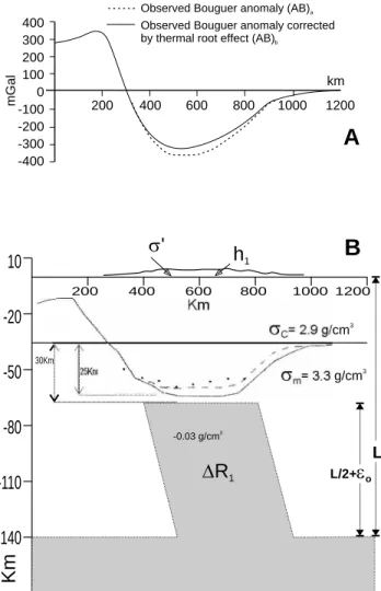
(11) mGal. Boletín del Instituto de Fisiografía y Geología 71(1-2), 2001.. 400 300 200 100 0 -100 -200 -300 -400. Observed Bouguer anomaly (AB)a Observed Bouguer anomaly corrected by thermal root effect (AB)b. 600. 800. 1000. 1200. (4) Great crustal increasing in thickness and width have been found out from the observed Bouguer anomalies on 22°S and 24.5°S latitudes. Using them, we have computed great rough shortenings of 420 km and 380 km respectively.. s' 200. 400. h1 600. 800. B. Acknowledgements This work has been supported by the following grants: (1) PID-BID N 214 (CONICET), and (2) "Programa de Fomento a la Investigación Científica y Tecnológica" Resol. N 239/92 (Universidad Nacional de Rosario).. 1000 1200. Km. -20. -80. 400. A. 10. -50. From the mentioned heating, it is possible that partial melt and magmatic intrusion of 5% of the thermal root area, could exist. Finally, we point out that gravimetric models satisfying seismic depths (for example 60 km on 24.5°S latitude) are not the only ones, because of the well known ambiguities of the potential field.. km 200. sC= 2.9 g/cm. 3. 30Km. sm= 3.3 g/cm. 25Km. 3. -0.03 g/cm3. L. -110. 11. DR1. L/2+eo. Km. -140. Figure 7. A: Regional observed Bouguer anomaly on 24.5° S latitude and regional observed Bouguer anomaly corrected by the gravimetric effect due to the lithospherical thermal root; B: Crustal thicknesses correponding to Models 1 and 2 (see Fig. 1A-B). Note the consistence between the crustal thickness of Model 2 and the seismic data indicated by black points. Figura 7. A: Anomalía regional de Bouguer observada en latitud 24.5° S y anomalía regional de Bouguer corregida por el efecto gravimétrico de la raíz térmica litosférica; B: Espesores corticales correspondientes a los Modelos 1 y 2 (véase Fig. 1A-B). Notar la consistencia entre los espesores corticales del Modelo 2 y los datos sísmicos indicados por puntos negros.. very small, less than 10% of the Bouguer anomalies. This guarantees that the isostatic equilibrium state can be analyzed independently of the selected model. For 22°S and 24.5°S sections of this paper, the isostatic anomalies in continental zone -using an Airy system- are small, in general terms, respect to the Bouguer anomalies, pointing out a tendency to compensation. (3) For the section located at 24.5°S, the seismic crustal model with a maximum depth of 60 km is consistent with the gravimetric crustal model involving heating at the lower half of the lithosphere, combined with crustal shortening. Since lithospheric heating may be a regional phenomena, it would also affect the section located at 22°S. In this case, the classic model without heating would give a maximum Moho depth of 68 km and 63 km with a thermal root located at the lower half of the lithosphere.. REFERENCES Abriata J.C. and Introcaso A., 1990. Contribución gravimétrica al estudio de la transecta ubicada al sur de Bolivia. - Revista IGM Argentina 7: 8-19. Araneda M., Chong G., Götze H., Lahmeyer B., Schmidt S. and Strunk S., 1985. Gravimetric modelling of the Northern Chilean lithosphere (20°-26° South latitud). - Actas del Cuarto Congreso Geológico Chileno 1: 2/18-2/34. Birch F., 1961. The velocity of compressional waves in rocks to 10 kilobars, 2. - Journal of Geophysical Research 66(7): 2199-2224. Bowin C., Warsi W. and Milligan J., 1981. Free Air Gravity Anomaly Atlas of the World. - Wood Hole Oceanographic Institution, 38p. Cerrato A., 1975. Contribuciones a la Geodesia Aplicada. Instituto de Geodesia U.B.A., 47p. Dorman L.M. and Lewis B.T., 1972. Experimental Isostacy, 1. Theory of the determination of the Earth's Isostatic Response to a Concentrated Load. - Journal of Geophysical Research 75(17): 3357-3365. Draguicevic M., 1970. Carta gravimétrica de los Andes Meridionales e interpretación de anomalías de gravedad de Chile Central. - Departamento de Geofísica y Geodesia (Universidad Nacional de Chile), Publicación 93: 1-42. Fisher R.L. and Raitt R.W., 1962. Topography and structure of the Perú-Chile Trench. - Deep-Sea Research 9: 423-443. Fleitout L. and Froideveaux C., 1982. Tectonics and topography for lithosphere containing density heterogeneities. - Tectonics 1: 21-56. Froideveaux C. and Isacks B.L., 1984. The mechanical state of the lithosphere in the Altiplano-Puna segment of the Andes. - Earth and Planetary Sciences Letters 71: 305-314. Froideveaux C. and Ricard Y., 1987. Tectonic evolution of high plateaus. - Tectonophysics 134: 1-9. Giesse P. and Reutter K.J., 1987. Movilidad de los márgenes continentales activos en los Andes Centrales. Investigaciones alemanas recientes en Latinoamérica, Geología. - Deutsche Forschungsgemeinschaft (Bonn) and Instituto de Colaboración Científica (Tübingen): 35-38. Götze H., Schwarz G. and Wigger P.J., 1987. Investigaciones geofísicas en los Andes Centrales. In:.
(12) 12. Hubert-Miller (ed.): Investigaciones alemanas recientes en Latinoamérica. Geología. - Deutsche Forschungsgemeinschaft (Bonn): 44-49. Götze H., Lahmeyer B., Schmidt S., Strunk S. and Araneda M., 1990. Central Andes Gravity data base. - EOS 71(16): 401-407. Grow J.A. and Bowin C.O., 1975. Evidence for highdensity crust and mantle beneath the Chile Trench due to the descending lithosphere. - Journal of Geophysical Research 80(11): 1449-1458. Haak V. and Giesse P., 1986. Subduction induced petrological processes as inferred from MT, seismological and seismic observations in N-Chile and S-Bolivia. In: P. Giesse (ed.): Forschungsberichte aus der zentrales Anden (21°S-25°S) und ausdem Atlas-System (Marckko) 1981-85. - Berliner geowissenschaften Abhandlungen A66: 1-264. Hayes D.E., 1966. A geophysical investigation of the PeruChile Trench. - Marine Geology 4: 209-251. Introcaso A., 1991. El comportamiento isostático de los Andes Argentino-Chilenos. Actas del Segundo Congreso da Sociedade Brasileira de Geofisica 1: 160-164. Introcaso A. and Pacino M.C., 1988. Gravity Andean model associated with subduction near 24°25´ South Latitude. - Revista Geofísica 44: 29-44. Introcaso A. and Pacino M.C., 1992. Contribución parcial del sistema de Pratt al balance isostático del segmento andino comprendido entre 13° y 27° de latitud Sur. Segundo Congreso de Ciencias de la Tierra, Santiago de Chile, (Resúmen expandido): 1-5. Introcaso A., Pacino M.C. and Fraga H., 1992. Gravity, isostasy and Andean crustal shortening between latitudes 30° and 35°S. - Tectonophysics 205: 31-48. Introcaso A., 1993. Anomalous upper mantle beneath the Central Andes. Isostasy and Andean uplift. - Second Symposium on Andean Geodynamics (Oxford, September 1993), expanded abstract. Isacks B., 1988. Uplift of the Central Andean Plateau and Bending of the Bolivian Orocline. - Journal of Geophysical Research 93(B4): 3211-3231. Kono M., Fukao Y and Yamamoto A., 1989. Mountain building in the Central Andes. - Journal of Geophysical Research 94(B4): 3891-3905. Marquardt D., 1963. An algorithm for least-squares estimation on nonlinear parameters. - Journal Soc. Indust. Appl. Math. 11: 431-441. Megard F., 1978. Etude geologique des Andes du Peru Central. - Mémoire ORSTOM 86: 1-310. Nafe J.E. and Drake C., 1965. Interpretation Theory in Applied Geophysics. Grant & West., 436 p. Pacino M.C. and Introcaso A., 1987. Regional anomaly. INTROCASO - Anomalous upper mantle (Andes). determination using the upwards-continuation method. - Bolletino di Geofisica Teorica e Applicata 29(114): 113-122. Pardo M. and Fuenzálida A., 1988. Estructura cortical y subducción en Chile Central. - Actas Quinto Congreso Geológico Chileno 2: F247-F265. Porth R., Schmitz M., Schwarz G., Strunk S. and Wigger P., 1990. Data compilation along two sections of the Southern Central Andes. Fin Worksh: Structural Evolution Central Andes, May 1990, Cerlin, Abstract 94. Schmitz M., Wigger P., Araneda J., Giese R., Heinsohn D., Röwer P. and Viramonte J., 1993. The Andean Crust at 24° S Latitude. - Actas XII Congreso Geológico Argentino 3: 286-290. Sheffels B., Burchfiel B.C. and Molnar P., 1986. Deformational style and crustal shortening in the Bolivian Andes. - EOS Transactions AGU 44: 1241. Suárez G., Molnar P. and Burchfiel B.C., 1983. Seismicity, fault plane solutions depth of faulting and active tectonics of the Andes of Peru, Ecuador and Southern Colombia. - Journal of Geophysical Research 88: 10403-10428. Talwani M., Worzel J.L. and Landisman M., 1959. Rapid gravity computations for two dimensional bodies with application to the MNendocino Submarine fracture zone. - Journal of Geophysical Research 64(1): 49-58. Tellería G.J., 1992. Mapa de anomalías de Bouguer y regiones morfoestructurales de la República de Bolivia. - Ed. Instituto Geográfico Militar (Bolivia). Wigger P., Schimitz M, Araneda M., Asch G., Baldzuhn S., Giesse P., Heinsohn W.D., Martinez E., Ricaldi E., Röwer P. and Viramonte J., 1993. Variation in the crustal structure of the Southern Central Andes deduced from seismic refraction investigations. In Reutter K.J., Scheuber E. and Wigger P. (eds.): Tectonics of the Southern Central Andes: 23-28, Springer, Heidelberg. Wollard G.P., 1959. Crustal structure from gravity and seismic measurements. - Journal of Geophysical Research 64(10): 1521-1544. Wollard G.P., 1969. The earth's crust and upper mantle. Pembroke J. Hart edit., 736p. Wollard G.P., 1970. Evaluation of the isostatic mechanism and role of mineralogic transformation from seismic and gravity data. Earth and Planetary interiors 3: 484-498. Wuenschell P.C., 1955. Gravity measurements and their interpretation in South America between latitudes 15°S and 33°S. Columbia Univeristy Press..
(13)
Figure


+5


Documento similar