TítuloHierarchical organization of spatial and temporal patterns of macrobenthic assemblages in the tropical Pacific continental shelf

Texto completo

(1)Hierarchical organization of spatial and temporal patterns of macrobenthic assemblages in the tropical Pacific continental shelf Godínez-Domínguez, E.1,2 Freire, J. 2 Franco-Gordo, C. 1,2 González-Sansón, G.3 1. Centro de Ecología Costera, Centro Universitario de la Costa Sur, Universidad de Guadalajara. V Gómez Farías 82.. San Patricio-Melaque, Jalisco. México. 38980. 2. Departamento de Biología Animal, Biología Vegetal y Ecología. Universidad de A Coruña. Campus da Zapateira s/n. A. Coruña, España. 15071. egodinez@mail2.udc.es 3. Centro de Investigaciones Marinas, Universidad de La Habana. La Habana, Cuba.. Summary 1. Nowadays, studies focused to test a well-defined set of a priori hypotheses about spatial and temporal organization of assemblages in marine communities are scarce. 2. This study presents the first fully-developed application of a parsimonious approach for model selection based on the Kullback-Leibler information theory using multivariate data to determine the best spatial and temporal models among a set of a priori alternative models of a soft bottom macroinvertebrate community in the tropical Pacific continental shelf (from 10 to 90 m deep). 3. Besides of the determination of the most parsimonious model, the Akaike´s information criterion allows the exploration of the scale-dependent patterns of community organization and to determine hierarchical relations among the gradients considered. 4. Depth is the most conspicuous spatial gradient affecting macrofaunal assemblages, and the main discontinuity is located between 40 and 60 m. The degree of exposure is defined as a secondary gradient and it is only relevant in shallow waters. 5. Seasonal changes in the abundance along the bathymetric gradient of some portunid crabs and shrimps defined a process of seasonal recomposition, caused by a vertical shift of the community.. 1.

(2) Keywords; Akaike information criterion, model selection, benthic macroinvertebrate assemblage,. spatial. patterns,. temporal. patterns,. tropical. continental. shelf,. environmental gradients, hydroclimatic seasonality. Introduction. Ecological systems are characterized by spatial and temporal variations in the density of organisms and resources, and in the intensity of processes that affect them (Thrush et al. 1997). This heterogeneity represents both a difficulty for the design of field studies and statistical testing, and a challenge to describe the spatial structuring of populations, communities and ecosystems (Legendre 1993). The description of pattern is the description of variation, and the quantification of variation requires the determination of scales. The fact that there is no single correct scale or level at which to describe a system, does not mean that all serve equally well or that there are not scaling laws (Levin 1992). The determination of spatial and temporal patterns in single populations has been approached mainly using fractals (Sugihara & May 1990; Kostylev & Erlandson 2001), semivariograms or correlograms (Sokal & Oden 1978; Freire, González-Guarriarán & Olaso 1992; González-Gurriarán, Freire & Fernández 1993) or spectral analysis (Klyashtorin 2001; Kendall, Prendergast & Bjørnstad 1998). However, the possible existence of spatial or temporal subjacent hierarchical patterns in communities has not been sufficiently considered (GodínezDomínguez & Freire, in press). Soft-sediment habitats are not generally considered highly structured habitats, although they can support a high diversity (Coleman, Gason & Poore 1997; Thrush et al. 2001). However virtually every ecosystem will exhibit patchiness and variability on a range of spatial, temporal and organizational scales, with substantial interaction with other systems and influence of local stochastic events (Levin 1992). In spite that shrimps in the Mexican Pacific coast are the targets of one of the most important local fisheries, the spatial and temporal dynamics of the community that support the shrimp commercial species remain unknown. One of the most visible, direct impacts of trawling is the capture of non-target species in the nets, and in shrimp fisheries, the weight of the bycatch caught is grater than the weight of the commercially important species (Saila 1983). In the Mexican Pacific fishery, the impact of fishing 2.

(3) effort alone does not explain the high catch variability of the commercial shrimps (López-Martínez et al. 2002) nor the structural features of the macroinvertebrate community (Godínez-Domínguez, Freire & González-Sansón, in press), which makes necessary to search for the primary causes of the variability in populations and communities and the hierarchical relation among them. In this paper, we show that model selection approaches based in the theory of information as the Akaike´s information criterion AIC, can be used to analyze the scaledependent pattern of a community and determine parsimonious hierarchical spatial and temporal models of assemblage organization as proposed by Godínez-Domínguez & Freire (in press). Material and Methods. Study area The study area is located on the continental shelf of the central portion of the Mexican Pacific (Fig. 1). The continental shelf of this region is very narrow, comprising, up to the 200-m isobath, only 7-10 km (Filonov et al. 2000). The predominant surface current patterns in the study area are described by Wyrtki (1965) for the eastern Pacific Ocean, consisting of the two main phases: the first one is influenced by the California Current, and it is characterized by a cold water mass from January-February to AprilMay; the second phase is a period (July-August to November-December) influenced by the North Equatorial Countercurrent and characterized by a tropical water mass (Badan 1997; Filonov et al. 2000; Godínez-Domínguez et al. 2000; Franco-Gordo et al. 2001; Franco-Gordo, Godínez-Domínguez & Suárez-Morales 2001). A third phase is determined by a transition between both previous phases neither one dominating (Franco-Gordo, Godínez-Domínguez & Suarez-Morales 2002). Sampling Five cruises (DEM 1 to DEM 5) were carried out aboard the research vessel BIP-V, during consecutive phases of the main hydroclimatic patterns defined by the surface currents. Seven sampling sites were selected along the coast during each cruise and, at each site, four stations were defined by depth (20, 40, 60, 80 m) (Fig 1). The sampling stations were fixed by GPS and maintained during all the cruises. Tows were carried out with paired shrimp trawls with a mouth opening of 6.9 m, headline 3.

(4) height of 1.15 m and stretched-mesh size along the bottom of the seine of 38 mm, one on each side of the vessel. Tows duration was 30 min with mean velocity of 2 knots and distance and areas towed were estimated from GPS fixes. Due to the pseudoreplicate nature of the information obtained from simultaneous tows, data were pooled to obtain a normalized value of organisms by ha-1. The sampling order of the sites was randomly selected and all the samples from a same site were taken the same night in a random way. Samples were preserved on ice and processed immediately; organisms were identified taxonomically, counted and fresh weight by species was recorded. In the present study, the dominant invertebrate groups in catches (cnidarians, molluscs, crustaceans, and echinoderms) are considered. The temperature and salinity of the bottom mass of water (<1 m from bottom) were recorded with a CTD profiler (SBE-19), previously to the tows. Dissolved oxygen was determined in a sample of water taken with a van Dorn bottle. Data analysis Modeling assemblage patterns Two sources of variability for macrobenthic communities are recognized: depth, which is one of the most important gradients in both benthic and demersal habitats, and degree of exposure, including the consequences of physical disturbance forces that determine erosion and deposition patterns. The interaction of both gradients is also taken into consideration here testing if the exposure effect is restricted only to shallow areas. A set of hypotheses corresponding to different, competing models of spatial organization were considered and are showed in Figure 2. These models are based in three basic hypotheses: a) effect of depth gradient; three levels are proposed: no effect, differences among all the depth strata, and differences between the shallow (20 and 40 m), and deep strata (60 and 80 m). b) Degree of exposure (alongshore variability), with two levels of effects: no effect, differences between exposed and sheltered areas. c) Interaction between depth and exposure; some models include the possibility that exposure is only affecting in shallow waters. Spatial patterns were analyzed independently for each cruise The temporal models presented here assume that variability is restricted to time and no spatial heterogeneity is included. Temporal hypotheses are defined as follow:. 4.

(5) -Model t1: community organization is similar in the different cruises (DEM 1=2=3=4=5). No temporal patterns are identified due to assemblage invariance. -Model t2: community organization is different in each cruise (DEM 1≠2≠3≠4≠5). No temporal pattern is identified due to a permanent (non-seasonal) assemblage variability. -Model t3: community organization changes seasonally according to the hydrographic structure (transition period ≠ tropical period ≠ subtropical-template period ((DEM 1,4) ≠ (DEM 2,5) ≠ (DEM 3)). -Model t4: the results of the selection of the spatial models for each cruise indicate that spatial organization was similar in the tropical and subtropical-temperate period. According with this fact the following temporal model was tested: transition period ≠ tropical period = subtropical-temperate period; (DEM 1,4) ≠ (DEM 2,5,3).. The most parsimonious models were selected from the eight spatial and four temporal models by means of the procedure proposed by Godínez-Domínguez & Freire (in press). The method consists first in the definition of a priori alternative models, which should reflect a set of a priori hypotheses as described above. Alternative models are defined with the codification of dummy variables representing spatial or temporal groups in the matrix of independent variables (an example of coding files is showed in Godínez-Domínguez & Freire, in press). The second step consists in the determination of the fit of models to data using the trace value generated by a canonical correspondence analysis CCA (ter Braak 1996). The statistical significance of the model fitted is determined by means of a F-ratio of the sum of all canonical eigenvalues and the residual sum of squares. This test has a high sensitivity to all kinds of deviations from the null hypothesis (ter Braak & Šmilauer 1998). The residual sum of squares is defined by:. h. RSS = ( sum of all eigenvalue s) − ∑ tracei i =1. where h is the number of factors in the model (Legendre & Anderson 1999). The third step consists in the determination among the significant models of the best model using a parsimonious selection procedure named Akaike´s Information Criterion. In a CCA, as more environmental variables are included more variance will be extracted (inclusive in the case that these variables do not have any causal relationship with the assemblage pattern), so a criterion that balances the trace and the size of the independent matrix is necessary to find the best model. The principle of parsimony is 5.

(6) defined by the tradeoff between squared bias and variance (uncertainty) versus the number of estimable parameters (groups in a ordination model) in the model (Burnham & Anderson 1998). The maximized log-likelihood is a biased estimator of this expected log-likelihood and the asymptotic bias equals K, the number of free parameters in the model (Akaike 1973), hence:. [( )]. AIC = − 2 log L θˆ + 2 K This has became known as Akaike´s Information Criterion or AIC and it makes possible to combine estimation and model selection under a single theoretical framework of optimization (Anderson, Burnham & Thompson 2001). There is a simple transformation of the estimated residual sum of squares (RSS) to obtain the value of log. L. (θ) when using least squares estimation with normally distributed errors rather. than the likelihood method. For all standard linear models, we can take. 1 log [L (θˆ )] = − n log(σˆ 2 ) 2 were log = loge, n is sample size and σ2 = RSS/n. To avoid the bias in AIC estimates due the number of parameters and sample size relation, Sugiura (1978) derived a secondary variant of AIC:.  2 K ( K + 1) )  AIC c = AIC +    n − K −1  AICc is used when the ratio n/K < 40. Due to the fact that AIC c is measured on an relative scale, Burnham and Anderson (2001) recommended the computation of the AIC differences (∆i ) rather than the AIC values, over all candidate models in the set:. ∆ i = AIC i − min AIC In order to get a better measurement of the plausibility of each model, Akakike (1983) proposed exp (-½ Äi) as being the relative likelihood of the model. Burnham and. 6.

(7) Anderson (2001) normalized the above expression to a set of positive “Akaike weights” summing 1:.  ∆  exp  − i  2   wi = R  ∆  exp  − r  ∑ 2   r =1 As Äi is becoming larger, wi is becoming smaller and less plausible is model i as the actual best model based on the design and sample size used. A non-metric multidimensional scaling nMDS ordination procedure (Clarke 1993) was carried out for visual exploration of the significant (CCA, P<0.05) spatial ordination models. Species associations Similarity percentage analysis (SIMPER) (Clarke 1993) was used to determine the taxa contributing most to the dissimilarity between groups of the significant models fitted. All these analyses were done using the Bray-Curtis similarity coefficient (Clarke 1993) applied to fourth-root-transformed species-abundance data. Analyses were performed using the software package PRIMER (Clark & Warwick 1994). In cruises DEM 2,3 and 5, and DEM 1 and 4 respectively, the same spatial models were selected (see Results) differentiating assemblages along the bathymetric gradient areas. For both groups of cruises, assemblage similarity was compared between depth strata and among cruises using a 2-way ANOSIM (Clarke & Warwick 1994) to determine seasonal patterns in the species assemblage recomposition. Results. Modeling assemblage patterns In most of cruises, several spatial models have a significant fit (P<0.05) (Table 1). There were at least seven significant (P<0.05) or statistically valid spatial models for cruises DEM 1 and DEM 2 (Table 1). For DEM 3, five significant models were found. For the DEM 4 no one model was statistically significant. The results of the nMDS. 7.

(8) show that an adequate graphical ordination pattern could be identified with several models (Fig. 3). For this reason a model selection procedure was imperatively required, for determine the best model. The spatial structure of cruises showed a consistent seasonal pattern. During the transition periods (DEM 1 and 4) the best model fitted was the s2, and the model s5 was the best one in the rest of the seasons of tropical (DEM 2 and 5) and subtropicaltemperate affinity (DEM 3). According to the AIC-values rank of the spatial models, depth is the most conspicuous spatial gradient of the macrofaunal assemblages, and the main discontinuity is located between 40 and 60 m. The degree of exposure is defined as a secondary gradient and it is only relevant in shallow waters. The evidence of an interaction between depth and exposure was found for the three first cruises (according to AIC scores, see Table 1): model s3 in cruises DEM 1 and 3, and model s7 in cruise DEM 2. Temporal analysis showed that two models were significant. However the model t2 which assume differences among every cruise, was the most parsimonious (Table 1). Species abundance patterns Portunus xantussi affinis was the dominant species ranging from 26.9% (DEM 2) to 89.9% (DEM 4) of the number of organisms captured, but with important changes in abundance from 439.7 (DEM 2) to 7791.4 (DEM 4) individuals · ha-1 (Table 2). Following to P. xantussi affinis, there were a wide group of species constituted mainly by portunid crabs, Portunus spp, P. asper, shrimps (Trachypenaeus brevisuturae, Sicyonia disdorsalis, Solenocera florea, S. mutator, Farfantepenaeus brevirostris), stomatopods (Squilla hancocki, S. panamensis), and starfishes (Luidia foliolata, and Astropecten armatus). A complete species checklist can be found in Appendix 1. Species associations Species assemblages along the bathymetric gradient were well defined. S. mutator, S. hancocki and S. panamensis, Cantharus gatesi, one unidentified species of Amphinomidae, the sponge and hermit crab association, A. armatus and Bufonaria nana defined the deep assemblage (60 and 80 m). T. brevirostris and P. asper were representative of the shallow assemblage (20 and 40 m). Crab species as P. xantusii 8.

(9) affinis and Portunus spp. conform a predator group that occurred in all the depth range and constitute the most abundant species. These species typified both for similarity (Table 3) and dissimilarity (Table 4) among assemblages in most of the cases in all the cruises and depth strata. During the transition periods, both crab species showed the highest abundances in the deep stratum; in the other hydroclimatic seasons the highest abundances were obtained at 40 or 60 m. During both transition periods (DEM 1 and 4), maximum abundances occurred in the deep stratum (Fig 4). During cruises DEM 2,3 and 5, maximum abundances where found deep strata (40 and 60 m). A differential trend during the DEM 3 (subtropical-template affinity) in relation to cruises carried out during the tropical season (DEM 2 and 5) was found for Portunus spp., P. asper, S. disdorsalis, S. disedwarsi and T. brevisuturae, whose highest abundances were located in shallow waters (20 and 40 m). Seasonal changes in the abundance along the bathymetric gradient of some portunid crabs and shrimps defined a process of seasonal recomposition, caused by a vertical shift of the community. A different bathymetric pattern was observed in the tropical and subtropical-temperate seasons, while during the transition period the depth gradient was less evident. During the subtropical-temperate period, the complete macroinvertebrate assemblage shifted towards shallow waters, while during the tropical period the assemblage moved to deeper waters. The presence during the subtropicaltemperate period at the deepest stratum of low-oxygen level tolerant species like S. mutator (see Hendrickx 1996) clearly demonstrates the existence of seasonal bathymetric movements. A few species characterized assemblages corresponding to sheltered and exposed areas and only two were abundant, F. californiensis typified the sheltered shallow waters and Arenaeus mexicanus the exposed sites, both in just two cruises (Table 5). The rest of species that typified for sheltered or exposed sites were rare as P. depresus, D. sinistripes and A. pulvinata. Although the same spatial model was selected for cruises DEM 2,3 and 5, differences in species assemblages among them could exist due to differences in their hydroclimatic affinity (DEM 2 = DEM 5. DEM 3). The ANOSIM test results indicate that. there was a significant difference between depth strata (R = 0.643), but no differences among cruises (R = -0.021, a negative value of R indicates higher assemblage 9.

(10) variability within the cruises than among them). A nMDS ordination showed these patterns (Fig 5). Similar results were obtained in the comparison between the two cruises (DEM 1 and 4) carried out during the hydroclimatic transition season, being the difference between depth strata statistically significant (R = 0.581) whereas between cruises the difference was not significant (R = - 0.250). Discussion. A wide range of spatial models were significant in several cruises, and in some cases they supported contradictory assumptions. According to the nMDS ordinations (Fig. 3) of these models, in the absence of a selection criterion any of these models could be assumed as valid and any hypotheses could be presented as final conclusions. The AIC is the only statistical tool currently available to compare models of ecological communities (Godínez-Domínguez & Freire in press). In fact, using other statistical procedures, different patterns could be obtained with the same data set when it is analyzed using different multivariate methods (Anderson & Clements 2000), and actually no discussion or justification about the selected method is required usually for publication. Perhaps the main contribution of the use of the AIC for model selection in community data is the determination of the most parsimonious one; however the possibility of exploration of the scale-dependent patterns constitute a powerful tool to analyze the hierarchical relation between the gradients implied. The order of the significant models in each cruise indicated by AIC values, could be interpreted as a rank of spatial scale-dependent patterns, or a hierarchical spatial pattern of assemblage organization (see Table 1), and should be considered not only in the design of future surveys but also to redefine the conception of the hierarchical gradients and of the subjacent variables. It means that depending of the scale and the region of the gradients, the patterns will be evidenced in different ways. Also, this approach allowed us to avoid the traditional disjunctive analysis strategy, which only could find a unique model without testing the alternatives (Godínez-Domínguez & Freire in press). The spatial structure found is determined by the relation between the two main physiographic traits in the coastal shelf; depth and exposure gradients (GodínezDomínguez & Freire in press), and a seasonal pattern related to the hydroclimatic processes that constitutes the main driving force for assemblage recomposition and spatial shift. Both depth and exposure are considered as complex gradients underlying other simpler ones. Bianchi (1992) defines depth as a spurious variable as it entails all 10.

(11) other possible factors varying along the water column (temperature, oxygen, salinity, pressure, light intensity, etc). Depth has been widely reported as the principal gradient in macrobenthic spatial distribution (Bianchi 1991; 1992; Basford, Eleftheriou & Raffaelli 1989). The exposure gradient encloses environmental variables as currents that could determine differential patterns in erosion and sediment deposition and, as a consequence, the type of seabed (Snelgrove & Butman 1994). The role of sediment type as a factor determining macrobenthic community patterns has been emphasized by several authors (Sanders 1958; Gray 1974). The exposure gradient was only relevant at shallow waters, and only during the first three cruises, the models that consider the interaction depth-exposure were significant. The decrease in the differences between exposed and sheltered areas in the shallow assemblage during the last two cruises could be related to complex changes in environmental and habitat conditions. There are several factors that favour the environmental differentiation between exposed and sheltered sites in the coastal soft bottoms. According to Blaber & Blaber (1981) the shallow zones of tropical areas act as nursery zones, which make these areas as ecologically conspicuous habitats (Longhurst & Pauly 1987). Despite that sedimentary aspects are important to explain diversity of the soft-bottom macrofauna, habitat structure explain better the positive relation with macrobenthic diversity (Thrush et al. 2001), and the relative importance of physical and biological elements of habitat structure vary with spatial scale. Differences between exposed and sheltered sites were not detected in deep areas including the cruises when exposure gradient was significant. No differences between the exposed and sheltered sites were detected for the temperature, salinity and dissolved oxygen (Fig 6). Jesse (1996), working with the soft-bottom macrocrustacean community in the continental shelf of Costa Rica, where a large number of species are shared with the present study, concluded that the species are adapted to strong environmental gradients and their occurrence is more dependant on substrate composition than on oceanographic conditions. The rain could be a significant factor to define substrate composition because determines the main sources of freshwater and organic matter. In fact, some areas contiguous to river mouths could change dramatically during the rain season because perturbed mud could be defaunated. Although ephemeral mouths are located in both bays and open beaches of the study area, the differential oceanographic dynamics during rain seasons in sheltered areas and the high-energy coastline (open beaches) produces differences on seabed environments. The cruise DEM 5 was carried out 11.

(12) towards the end of the rain season but DEM 4 was carried out during the dry season, so the rain factor (salinity and terrestrial organic matter) could not explain alone the homogeneity of the shallow assemblage. In fact during DEM 4 neither depth nor exposure were identified as significant gradients and it could be hypothesized that a strong, unrecorded, environmental disturbance generated the loss of community spatial structure. A large mud disturbance is discarded due to the low oxygen values obtained during rain seasons. The loss of spatial structure could not be attributed to fishing disturbance because the DEM 4 was carried out towards the end of the close season (Godínez-Domínguez, Freire & González-Sansón, in press), without fishing pressure for almost three months. The organization in space and time of the macrobenthic assemblages in the shelf of the tropical Pacific could be explained using the concept of the continuum (Mills 1969). Apparently homogeneous habitats are occupied by an assemblage that responds to the local hydroclimatic dynamics (Godínez-Domínguez, Freire & GonzálezSansón, in press) with a seasonal bathymetric shift forcing species recomposition. The labile gradient of exposure found at shallow waters, could be related to the environmental instability of the zone where during some periods, the substrate from sheltered and exposed areas could be similar, but differences could be apparent in other periods. According to Darnell (1990), the interior shelf is characterized through high-energy flows, tidal cycles and current patterns that cause a dynamic water column. Acknowledgements. To the staff of the “demersal program” of the University of Guadalajara and to the crew of the research vessel BIP V, Celestino Preciado Gudiño, Salomon Medina Morales, and Daniel Kosonoy Aceves. To Victor Landa Jaime and Rafael García de Quevedo Machaín who helped with the taxonomical identification of the organisms, and Michael Hendrickx who validated crustaceans group. Research was partially founded by the University of Guadalajara, México, by the Consejo Nacional de Ciencia y Tecnología CONACyT Mexico, and by the grant REN2000-0446 from the Spanish Ministerio de Ciencia y Tecnología.. 12.

(13) References. Akaike, H. (1973) Information theory as an extension of the maximum likelihood principle. In Petrov BN, Csaki F (eds). Second International Symposium on Information Theory. Akademiai Kiado, Budapest, pp 267-281. Akaike, H. (1983) Information measures and model selection. International Statistical Institute, 44, 277-291.. Anderson, D.R., Burnham, K.P. & Thompson, W.L. (2001) Null hypothesis testing: problems prevalence and an alternative. Journal Wildlife Management, 64, 912923. Anderson, M.J. & Clements, A. (2000) Resolving environmental disputes: a statistical method for choose among competing cluster models. Ecological Applications., 10, 1341-1355. Badan, A. (1997) La Corriente Costera de Costa Rica en el Pacífico mexicano. Monogr. No. 3 Unión Geofísica Mexicana, pp. 99-112. Basford, D.J., Eleftheriou, A. & Raffaelli, D. (1989) The epifauna of the northern North Sea (56°-61° N). Journal of the Marine Biological Association of the United Kingdom, 69, 387-401. Bianchi, G. (1991) Demersal assemblages of the continental shelf and slope edge between the Gulf of Tehuantepec (Mexico) and the Gulf of Papagayo (Costa Rica). Marine Ecology Progress Series, 73, 121-140. Bianchi, G. (1992) Study of the demersal assemblage of the continental shelf and upper slope off Congo and Gabon, based on the trawl surveys of the RV “Dr Fridtjof Nansen”. Marine Ecology Progress Series, 85, 9-23.. Blaber, S.J.M. & Blaber, T.G. (1981) The zoogeographical affinities of estuarine fishes in South-East Africa. South African Journal of Science, 77, 305-307.. 13.

(14) Burnham, K.P. & Anderson, D.R. (1998) Model selection and inference. A practical information-theoretic approach. Springer-Verlag, New York, 353 pp. Burnham, K.P. & Anderson, D.R. (2001) Kullback-Leibler information as a basis for strong inference in ecological studies. Wildlife Research, 28, 111-119 Clarke, K.R. (1993) Non-parametric analyses of changes in community structure. Australian Journal of Ecology, 18,117-143. Clarke, K.R. & Warwick, R.M. (1994) Change in marine communities: an approach to statistical analysis and interpretation. Plymouth Marine Laboratory, Plymouth Coleman, N., Gason, A.S.H. & Poore, G.C.B. (1997) High species richness in the shallow marine waters of south east Australia. Marine Ecology Progress Series, 154, 17-26 Darnell, R.M. (1990) Mapping of the biological resources of the continental shelf. American Zoologist, 30, 15-21. Filonov, A.E., Tereshchenko, I.E., Monzón, C.O., González-Ruelas, M.E. & GodínezDomínguez, E. (2000) Variabilidad estacional de los campos de temperatura y salinidad en la zona costera de los estados de Jalisco y Colima, México. Ciencias Marinas, 26, 303-321. Franco-Gordo, C., Suárez-Morales, E., Godínez-Domínguez, E. & Flores-Vargas, R. (2001) A seasonal survey of the fish larvae community of the central Pacific coast of Mexico. Bulletin of Marine Science, 68, 383-396.. Franco-Gordo, C., Godínez-Domínguez, E. & Suárez-Morales, E. (2001) Zooplancton biomass variability in the Mexican Eastern Tropical Pacific. Pacific Science, 55, 191-202. Franco-Gordo, C., Godínez-Domínguez, E. & Suárez-Morales, E. (2002) Larval fish assemblages in waters off the central pacific coast of Mexico. Journal Plankton Research, 24, 775-784.. 14.

(15) Freire, J., González-Gurriarán, E. & Olaso, I. (1992) Spatial distribution of Munida intermedia and M. Sarsi (Crustacea: Anomura) on the Galicia continental shelf (NW Spain): application of geostatistical analysis. Estuarine Coastal & Shelf Science, 35, 637-648.. Godínez-Domínguez, E., Rojo-Vázquez, J., Galván-Piña, V. & Aguilar-Palomino, B. (2000) Changes of structure of a coastal fish assemblage exploited by small scale gillnet fisheries during an El Niño-La Niña event. Estuarine Coastal & Shelf Science, 51, 773-787. Godínez-Domínguez E, Freire J (in press) An information-theoretic approach for selection of spatial and temporal models of community organization. Marine Ecology Progress Series Godínez-Domínguez, E.,. Freire, J. & González-Sansón, G. (in press) Fishing. disturbance in the macroinvertebrate community of a shrimp fishing ground at Mexican central Pacific. Journal of Experimental Biology & Marine Ecology González-Gurriarán, E., Freire, J. & Fernández, L. (1993) Geostatistical analysis of spatial distribution of Liocarcinus depurator, Macropipus tuberculatus and Polybius henslowii (Crustacea: Brachyura) over the Galician continental shelf (NW Spain). Marine Biology, 115, 453-461 Gray, J.S. (1974) Animal-sediment relationships. Oceanography & Marine Biology Annual Review, 12, 223-261 Hendrickx, M.E. (1996) Los camarones Penaeoidea bentónicos (Crustacea: Decapoda: Dendrobranchiata) del Pacífico mexicano. Comisión Nacional para el Conocimiento y Uso de la Biodiversidad e Inst. Cienc. Mar y Limnol., UNAM, México. 148 pp. Jesse, S. (1996) Demersal crustacean assemblages along the Pacific coast of Costa Rica: a quantitative and multivariate assessment based on the Victor Hansen Costa Rica Expedition (1993/1994). Revista de Biología Tropical, 44, Supl 3, 115-134. 15.

(16) Kendall, B.E., Prendergast, J. & Bjørnstad, O.N. (1998) The macroecology of population dynamics: taxonomic and biogeographic patterns in population cycles. Ecological Letters 1, 160-164. Klyashtorin, L.B. (2001) Climate change and long-term fluctuations of commercial catches: the possibility of forecasting. FAO fish tech pap, 410, 86 p. Kostylev, V. &. Erlandsson, J. (2001) A fractal approach for detecting spatial. hierarchical and structure on mussel beds. Marine Biology, 139, 497-506 Legendre, P. (1993) Spatial autocorrelation: trouble or new paradigm? Ecology 74, 1659-1673 Lengendre, P. & Anderson, M.J. (1999) Distance-based redundancy analysis: testing multispecies responses in multifactorial ecological experiments. Ecological Monograph, 69, 1-24 Levin, S.A. (1992) The problem of pattern and scale in ecology. Ecology, 73, 19431967. López-Martínez, J., Arreguín-Sánchez, F., Hernández-Vázquez, S., Herrera-Valdivia, E. & García-Juárez, A.R. (2002) Dinámica poblacional del camarón café Farfantepenaeus californiensis (HOLMES, 1900) en el Golfo de California: Variabilidad interanual. Contributions of the study of the East Pacific Crustaceans (ed M. Hendricks). Vol 1, UNAM, 347 pp. Longhurst, A.R. & Pauly, D. (1987) The ecology of tropical oceans. Academic Press, Orlando, Florida. Mills, E.L. (1969) The community concept in marine zoology with comments on continua and instability in some marine communities. A review. Journal of the Fisheries Research Board of Canada, 26, 1415-1428 Saila, S.A. (1983). Importance and assessment of discards in commercial fisheries. FAO Fish Circ No 765, 62 pp. 16.

(17) Sanders, H.L. (1958) Benthic studies in Buzzards Bay. I. Animal sediment relationships. Limnology & Oceanography, 3, 245-258 Snelgrove, P.R.V. & Butman, C.A. (1994) Animal-sediment relationships revisited: cause versus effects. Oceanography & Marine Biology Annual Review, 32, 11177 Sokal, R.R. & Oden, N.L. (1978) Spatial autocorrelation in biology 2: some biological implications and four examples of evolutionary and ecological interest. Biological Journal of the Linnean Society, 10, 229-249.. Sugihara, G. &. May,. R.M. (1990) Applications of fractals in ecology. Trends in. Ecology & Evolution, 5, 79-86.. Sugiura, N. (1978) Further analysis of the data by by Akakike´s information criterion and the finite corrections. Communications in Statistics, Theory & Methods, 7, 13-26 ter Braak, C.J.F. (1996) Unimodal models to relate species to environment. DLOAgricultural Mathematics Group, Wageningen. ter Braak, C.J.F. Šmilauer, P. (1998) CANOCO reference manual and user´s guide to Canoco for Windows; software for canonical community ordination (version 4.0). Microcomputer Power (Ithaca, NY, USA), 352 pp. Thrush, S.F., Pridmore, R.D., Bell, R.G., Cummings, V.J. & 16 others (1997) The sandflat habitat: scaling from experiments to conclusions. Journal of Experimental Marine Biology & Ecology, 216, 1-9. Thrush, S.F., Hewitt, J.E., Funnell, G.A., Cummings, V.J. & 4 others (2001) Fishing disturbance and marine biodiversity: role of habitat structure in simple softsediments systems. Marine Ecology Progress Series, 221, 255-264 Wyrtki, K. (1965) Surface currents of the Eastern Tropical Pacific Ocean. InterAmerican Tropical Tuna Commission Bulletin, IX, 271-304. 17.

(18) Figure captions Figure 1. Study area. Sampling sites are shaded. Figure 2. Schematic representation of the hypotheses tested about the spatial community organization. Each box represents samples with homogeneous community structure. Figure 3. Ordination obtained by nMD S for each cruise and spatial model. Only the statistically significant models (CCA, P<0.05) are showed (three in cruises DEM 1, 2 and 3, ordered by their rank obtained from AIC, and only on in DEM 5), except in cruise DEM 4 in which no model was significant and only the first model ranked by AIC is showed. Numbers in each plot correspond to the different spatial boxes showed in Fig 2. Figure 4. Patterns of abundance of the dominant species in each cruise and depth strata. For cruises DEM 1 and DEM 4, deep (60 and 80 m) and shallow (20 and 40 m) strata were differentiated, in DEM 1, 2 and 3 the four strata were represented. Figure 5. Ordination obtained by nMDS of the macroinvertebrate assemblages of groups of cruises with similar spatial organization: model s5 for DEM 1 and DEM 2, and model s2 for DEM 2, 3 and 5. Polygons group samples from each depth strata. Figure 6. Temperature, salinity and dissolved oxygen profiles for the different cruises in each depth strata and along the exposure gradient. No dissolved oxygen data were recorded in cruises DEM 1 and 2.. 18.

(19) a hí Ba. a tit ca a n Te. a hí Ba. México. ad vid a N. a hí Ba. go tia n Sa. a hí Ba. illo an z an M. na gu a L. de. n lá ut y Cu. 19° N 105° W. Pacific Ocean. N 0. Figure 1. Godínez-Domínguez et al.. 5. 10 km.

(20) sheltered. exposed. 20 Model s1. Model s2. depth. 40 60 80. Model s3. Model s4. Model s5 Model s6. Model s7. Figure 2. Godínez-Domínguez et al.. Model s8.

(21) DEM 1. Model 2. Model 3. 1 2 1 1 2 22 1 1 1 1 1 1 222 22 22 1 11 22 1 1. 2 3 2 1 3 33 2 2 2 2 1 1 333 33 33 1 11 33 1 1. 2. DEM 2. 1 3 2 2 3 33 2 2 1 1 2 2 444 34 33 1 12 44 1 1. 3. Model 7. 23 2 3 3 3 2 2 33 4 1 1 4 1 1 4 2 2 1 4 44 4 1. 45 4 5 5 5 3 4 55 6 1 2 6 1 1 6 3 3 2 6 66 6 1. 12. 23. Model 5. Model 2. 2 3 33 4 2 1 222 3 3 1 4 1 1 2 23 3 4 4 1 4 4 1 4 1. 1 2 22 2 1 1 111 2 2 1 2 1 1 1 12 2 2 2 1 2 2 1 2 1. Figure 3. Godínez-Domínguez et al.. DEM 4. Model 2. 4. Model 5. DEM 3. Model 5. Model 2. 12 1 2 2 2 1 1 22 2 1 1 2 1 1 2 1 1 1 2 22 2 1. 1 1 2 1 22 1 2 22 2 2 1 2 22 1 1 1 11 2 1 2 2 1 11. 11. Model 3. 2 3 33 3 2 2 121 3 3 1 3 1 1 1 13 3 3 3 1 3 3 2 3 2. DEM 5. Model 5. 32 21 3 3322 3 2 44 4 3 2 1 44 1 1 44 3 2 1 1 1.

(22) Amphinomidae. Astropyga pulvinata. 80. 400 DEM 1 DEM 4. DEM 2 DEM 3 DEM 5. 300. 200. DEM 2 DEM 3 DEM 5. 40. DEM 1 DEM 4 20. 200 10. 100. 0. 0. 0 0. 20. 40. 60. 80. shallow. deep. 20. 40. Number of individuals ha-1. 200. DEM 5. shallow. deep. 240. 160. 160 DEM 2 DEM 3. 80. Farfantepenaeus brevirostris. Sponge and hermit crab 240. 60. DEM 2 DEM 3 DEM 5. DEM 1 DEM 4 120. 120. 200. DEM 1 DEM 4. 160 160. 80. 80. 120 80. 120 80. 40 40. 40. 40 0. 0. 0 20. 40. 60. 0. 80. shallow. 20. deep. 40. 60. Pleuroncodes planipes 900. shallow. deep. Portunus asper. 1.0. 1200. 80. 400. DEM 2 DEM 3 DEM 5. DEM 1 DEM 4. DEM 2 DEM 3 DEM 5. 300. DEM 1 DEM 4. 240. 180 600. 200. 0.5. 120 300. 100 60. 0. 0 0.0 20. 40. 60. 0. 80. shallow. 20. deep. 40. 60. Portunus xantusii affinis DEM 2 DEM 3 20000 20000 DEM 5. shallow. deep. Portunus spp 800. 1600. 24000 24000. 4000. 80. DEM 2 DEM 3 DEM 5. DEM 1 DEM 4. 1200. 700. DEM 1 DEM 4. 600. 16000 16000. 500 2000. 12000 12000 8000. 8000. 4000. 4000. 800. 400 300. 400. 0. 0 20. 40. 60. 80. 200. 0. 100. 0 shallow. Depth (m) Figure 4. Godínez-Domínguez et al. (1 of 2). deep. 20. 40. 60. Depth (m). 80. 0 shallow. deep.

(23) Sicyonia disdorsalis. Sicyonia disedwardsi 180. 300. DEM 2 DEM 3 DEM 5. 240 180. 200. DEM 1 DEM 4. DEM 2 DEM 3 DEM 5. 160. 120. 120. 120. 80. 60. 40. 0. 0. 200. DEM 1 DEM 4. 160 120. 60. 80 40. 0. 20. 40. 60. 0. 80. shallow. deep. 20. 40. 60. 80. Solenocera florea DEM 2 DEM 3 DEM 5. Number of individuals ha-1. 800. 120 100. 140. DEM 2 DEM 3 DEM 5. 120. 60. 200. 40. DEM 1 DEM 4. 100. 80. 400. deep. Cantharus gatesi. 240 DEM 1 DEM 4 180. 600. shallow. 80. 120. 60 40. 60 20. 20. 0 0 20. 40. 60. 0. 80. shallow. 0. deep. 20. 40. 60. 80. Solenocera mutator 4000. shallow. deep. Squilla hancocki. 1.0 DEM 2 DEM 3 DEM 5. DEM 1 DEM 4. DEM 2 DEM 3 DEM 5. 600. 160. 400. 120. 200. 80. DEM 1 DEM 4. 2000 0.5. 40. 0. 0 0.0 20. 40. 60. 0 shallow. 80. 20. deep. 40. 60. Squilla panamensis 1200. DEM 2 DEM 3 DEM 5. 400. 80. deep. Trachypenaeus brevisuturae 1000. DEM 1 DEM 4. DEM 2 DEM 3 DEM 5. 800. DEM 1 DEM 4. 200 160. 300. 800. shallow. 600 200. 400. 120. 400. 80. 200. 100 0. 40. 0 0 20. 40. 60. Depth (m) Figure 4. (2 / 2). 80. shallow. deep. 0 20. 40. 60. Depth (m). 80. shallow. deep.

(24) a). DEM 1 DEM 4 20 m 40 m 60 m 80 m. b). DEM 2 DEM 3 DEM 5 20 m 40 m 60 m 80 m. Figure 5. Godínez-Domínguez et al..

(25) 30 34.8. DEM 1. 25. 34.6 34.4 34.2. 20. O. 34 15 0. 20. 40. 60. 80. 100. 33.6. 30. 20. 40. 60. 0. 20. 40. 60. 0. 20. 40. 60. 0. 20. 40. 60. 80. 100. 34.6 34.4 34.2. 20. 34. DEM 2. 33.8. 0. 20. 40. 60. 80. Salinity. 15 100 6. 30. 5. DEM 3. 25. DEM 3. 4 3 2. 15 20. 40. 60. 80. 100. 2. 0. l-1. 20. 30. 40. 60. 80. 100. 20. 40. 60. 80. DEM 3. 33.6 80. 100. 34.8. DEM 4. 34.6 34.4. 3. 34.2. 2. 34. 33.6. 0. 100. DEM 4. 33.8. 0 0. 34.2. 6. 1 15. 34.4. 34. 20. 100. 34.6. 33.8 0. 80. 34.8. 0. 4. 20. 33.6. 1. 5. DEM 4. 25. mg. Temperature ° C. 0 34.8. DEM 2. 25. DEM 1. 33.8. 20. 40. 60. 80. 100. 80. 100. 6. 30. 34.8. 25. exposed. 5. exposed. sheltered. 4. sheltered. 34.6. 20. 34.2. 2. DEM 5. 34. DEM 5. 1. 15 20. 40. 60. 80. Depth m Figure 6. Godínez-Domínguez et al.. 100. exposed. 33.8. sheltered. 33.6. 0 0. DEM 5. 34.4. 3. 0. 20. 40. 60. Depth m. 80. 100. 0. 20. 40. 60. Depth m. 80. 100.

(26) Table 1. Results of the procedure applied for the selection of spatial and temporal models using the Akaike information criterion (AIC) and the significance of the canonical correspondence analyses carried out. For spatial models, the sample size (n) by cruise was 28. For temporal models n = 140.. cruise DEM 1 total inertia = 2.857 trace w P-value first canonical axis P-value global test DEM 2 total inertia = 4.556 trace w P-value first canonical axis P-value global test DEM 3 total inertia = 4.812 trace w P-value first canonical axis P-value global test DEM 4 total inertia = 2.550 trace w P-value first canonical axis P-value global test DEM 5 total inertia = 4.455 trace w P-value first canonical axis P-value global test K (number of parameters). total inertia = 6.218 trace w P-value first canonical axis P-value global test K (number of parameters). Spatial models s4 s5. s1. s2. s3. 0.065 0.011. 0.652 0.291. 0.814. 0.001. 0.821 0.252 0.001 0.001. 0.865 0.087 0.001 0.001. 0.284 0.053. 0.497 0.109. 0.529. 0.001. 0.797 0.091 0.006 0.001. 0.204 0.116. 0.489 0.283. 0.333. 0.001. 0.047 0.259. 0.082 0.316. 0.774. 0.082. 0.036 0.170. 0.213 0.302. 0.986 2. 0.225 2. t1 0.000 0.226. 1. s6. s7. s8. 0.979 0.199 0.001 0.001. 1.058 0.081 0.001 0.001. 1.242 0.072 0.001 0.001. 1.408 0.007 0.001 0.001. 1.081 0.069 0.011 0.002. 1.503 0.425 0.001 0.001. 1.094 0.016 0.043 0.023. 1.940 0.162 0.001 0.001. 2.444 0.073 0.001 0.001. 0.657 0.140 0.006 0.009. 0.890 0.080 0.004 0.008. 1.251 0.308 0.001 0.001. 0.955 0.023 0.150 0.128. 1.520 0.040 0.010 0.007. 2.046 0.010 0.108 0.006. 0.119 0.111 0.560 0.620. 0.155 0.035 0.790 0.830. 0.419 0.178 0.050 0.077. 0.514 0.076 0.163 0.179. 0.590 0.025 0.190 0.140. 0.653 0.001 0.324 0.437. 0.225 0.089 0.530 0.742 3. 0.367 0.037 0.394 0.704 4. 0.981 0.357 0.001 0.003 4. 0.402 0.009 0.858 0.852 5. 1.157 0.032 0.001 0.053 6. 1.479 0.003 0.011 0.140 8. Temporal models t2 t3 t4 0.180 0.410 0.058 0.222 0.397 0.155 0.001 0.008 0.001 0.013 0.165 3 5 2.

(27) Table 2. Frecuency of occurrence (%) and abundance (no · ind · ha-1) for the dominant species in each cruise.. Cruise DEM 1 Portunus xantusii affinis Trachypenaeus brevisuturae Sicyonia disdorsalis Luidia foliolata Sponge and hermit crab Solenocera florea Portunus asper Squilla hancocki Harpa crenata Amphinomidae Loliolopsis diomedae Cantharus gatesi Arenaeus mexicanus Ficus ventricosa Astropecten armatus Paradasygyus depresus Portunus spp. Renilla kollikeri Bufonaria nana Fusinus dupetitthouarsi Sicyonia martini Euphylax robustus Sicyonia disedwardsi Iliacantha hancoki. abundance. SD. 64.3. 779.9. 1479.4. 4.6. 55.4. 112.5. 3.1. 37.5. 127.5. 3.0. 36.5. 78.2. 2.9. 35.1. 102.9. 2.0. 24.4. 50.0. 2.0. 24.2. 54.8. 1.4. 17.2. 28.1. 1.1. 13.9. 36.5. 0.9. 11.2. 41.3. 0.9. 11.1. 28.9. 0.9. 10.7. 26.9. 0.9. 10.5. 21.3. 0.9. 10.4. 16.8. 0.8. 9.4. 18.5. 0.8. 9.3. 17.1. 0.7. 8.1. 30.2. 0.7. 7.9. 37.0. 0.6. 7.7. 11.7. 0.6. 7.4. 17.7. 0.6. 7.0. 21.4. 0.5. 6.0. 19.0. 0.5. 5.8. 15.0. 0.5. 5.6. 10.0. Frecuency. abundance. SD. 89.8. 7791.4. 11343.2. 2.9. 252.5. 414.2. 1.2. 100.4. 302.5. 0.7. 63.8. 161.9. 0.6. 53.4. 96.3. 0.5. 43.2. 149.7. Cruise DEM 4 Portunus xantusii affinis Portunus spp. Squilla panamensis Portunus asper Squilla hancocki Farfantepenaeus brevirostris. Cruise DEM 2. Mean Frecuency. Portunus xantusii affinis Solenocera mutator Portunus spp. Trachypenaeus brevisuturae Squilla hancocki Portunus asper Astropyga pulvinata Sicyonia disdorsalis Solenocera florea Sponge and hermit crab Farfantepenaeus brevirostris Cantharus gatesi Sicyonia martini Farfantepenaeus californiensis Luidia foliolata Squilla panamensis Amphinomidae Tubicolous polychaete Sicyonia disedwardsi. abundance. SD. 26.9. 439.7. 965.0. 19.1. 312.6. 1493.2. 16.7. 273.7. 524.9. 7.0. 115.3. 316.5. 5.4. 88.0. 289.0. 2.9. 47.0. 140.5. 2.6. 43.3. 138.1. 2.3. 37.6. 85.5. 2.1. 34.4. 62.0. 1.9. 30.7. 92.6. 1.8. 28.9. 63.8. 1.4. 23.7. 76.0. 1.3. 21.4. 81.7. 0.9. 14.6. 38.9. 0.9. 14.3. 30.3. 0.6. 10.6. 35.5. 0.6. 10.6. 50.8. 0.6. 9.9. 37.0. 0.5. 8.3. 21.5. Cruise DEM 5. Mean. Portunus xantusii affinis Solenocera mutator Portunus spp. Pleuroncodes planipes Squilla panamensis Squilla hancocki Portunus asper. Cruise DEM 3. Mean Frecuency. Mean Frecuency. abundance. SD. 85.3. 7341.0. 10355.1. 3.8. 323.7. 1493.7. 3.0. 260.7. 588.3. 1.3. 111.3. 470.1. 1.3. 109.4. 505.2. 1.1. 91.5. 263.9. 0.6. 47.3. 145.8. Mean Frecuency. Portunus xantusii affinis Portunus spp. Trachypenaeus brevisuturae Solenocera florea Solenocera mutator Squilla panamensis Tubicolous polychaete Sicyonia disdorsalis Portunus asper Amphinomidae Squilla hancocki Cantharus gatesi Sponge and hermit crab Astropyga pulvinata Metapenaeopsis beebei Sicyonia disedwardsi Astropecten armatus Sicyonia martini Ficus ventricosa Luidia foliolata Pleuroncodes planipes. abundance. SD. 41.5. 997.6. 1690.4. 12.3. 296.1. 560.3. 8.5. 204.5. 377.6. 6.4. 153.8. 354.7. 4.9. 118.8. 485.2. 4.4. 105.8. 409.4. 2.4. 57.4. 299.7. 1.8. 44.0. 113.2. 1.8. 42.9. 135.1. 1.5. 35.9. 86.5. 1.5. 35.0. 91.9. 1.3. 32.2. 70.4. 1.3. 30.3. 87.5. 1.2. 28.7. 151.4. 1.1. 25.3. 114.2. 1.0. 24.2. 80.3. 0.7. 17.0. 24.0. 0.5. 12.9. 32.7. 0.5. 12.3. 20.1. 0.4. 10.2. 15.3. 0.4. 9.2. 29.9.

(28) Table 3. Percentage contributions of species typifying similarity within each spatial group defined by the most parsimonious models in each cruise. Depth strata DEM 2 20 m Trachypenaeus brevisuturae Portunus asper Arenaeus mexicanus Luidia foliolata Astropyga pulvinata. 40 m. 60 m. 80 m. 25.89 12.89 12.09 9.99 9.32. Trachypenaeus brevisuturae Portunus asper Luidia foliolata Sicyonia disdorsalis Portunus spp. Portunus xantusii affinis Solenocera florea Dardanus sinistripes. 14.47 12.42 11.67 7.00 6.63 5.97 5.22 5.05. Portunus xantusii affinis Portunus spp. Solenocera florea Squilla hancocki Sicyonia martini Farfantepenaeus brevirostris Sicyonia disdorsalis. 16.06 15.44 10.03 7.82 6.23 5.76 5.40. Cantharus gatesi Portunus xantusii affinis Bufonaria nana Astropecten armatus Squilla panamensis Sponge and hermit crab Portunus spp. Fusinus dupetitthouarsi. 11.00 9.46 9.26 8.47 7.20 6.82 5.41 5.08. 16.63 14.95 9.92 8.80 7.56 5.07. Portunus xantusii affinis Portunus spp. Solenocera florea Ficus ventricosa Trachypenaeus brevisuturae Farfantepenaeus brevirostris. 14.23 9.41 9.01 5.67 5.47 4.65. Portunus xantusii affinis Squilla panamensis Solenocera florea Astropecten armatus Farfantepenaeus brevirostris Sponge and hermit crab Squilla hancocki. 12.16 7.73 7.56 7.26 5.83 5.79 5.32. Sponge and hermit crab Cantharus gatesi Astropecten armatus Portunus xantusii affinis Bufonaria nana Crucibulum lignarium Fusinus dupetitthouarsi. 12.87 12.49 11.05 10.76 10.37 6.87 6.65. 25.28 19.00 12.15 9.42 4.29. Portunus xantusii affinis Solenocera florea Dardanus sinistripes Squilla hancocki Portunus spp.. 41.20 8.49 8.00 7.28 6.60. Portunus xantusii affinis Squilla hancocki Squilla panamensis Farfantepenaeus brevirostris Fusinus dupetitthouarsi Bufonaria nana Astropecten armatus. 15.71 8.39 7.14 6.29 6.22 5.34 5.21. Solenocera mutator Cantharus gatesi Pleuroncodes planipes Bufonaria nana Fusinus dupetitthouarsi Astropecten armatus Sponge and hermit crab. 14.57 13.82 13.68 9.65 6.97 5.86 5.17. 15.08 8.28 7.93 6.69 6.56 5.87 5. Portunus xantusii affinis Solenocera florea Bufonaria nana Squilla hancocki Ficus ventricosa Paradasygyus depresus Iliacantha hancoki Astropecten armatus. 15.58 6.81 5.49 4.93 4.54 4.28 4.17 3.53. 18.01 13.23 11.39 7.90 6.39 6.11 5.00. Portunus xantusii affinis Squilla hancocki Portunus spp.. 30.22 8.66 6.72. DEM 3 Trachypenaeus brevisuturae Portunus xantusii affinis Portunus spp. Luidia foliolata Sicyonia disdorsalis Portunus asper. DEM 5 Portunus xantusii affinis Trachypenaeus brevisuturae Portunus asper Arenaeus mexicanus Dardanus sinistripes. DEM 1 20 and 40 m Trachypenaeus brevisuturae Arenaeus mexicanus Portunus xantusii affinis Loliolopsis diomedae Luidia foliolata Portunus asper Cycloes bairdii. 60 and 80 m. DEM 4 Portunus xantusii affinis Trachypenaeus brevisuturae Luidia foliolata Portunus asper Arenaeus mexicanus Dardanus sinistripes Portunus spp..

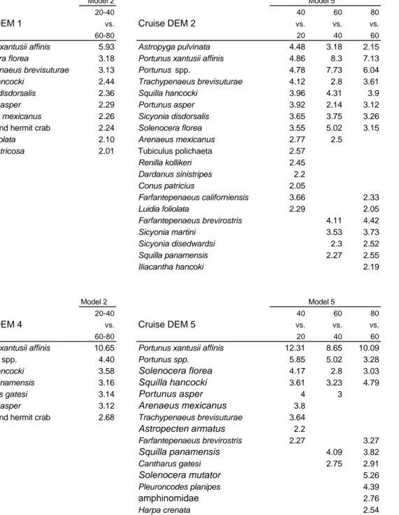
(29) Table 4. Percentage contributions of species typifying disimilarity among spatial groups defined by the most parsimonious spatial models of each cruise.. Model 2. Model 5. 20-40. Cruise DEM 1. vs.. Cruise DEM 2. 60-80. Portunus xantusii affinis Solenocera florea Trachypenaeus brevisuturae Squilla hancocki Sicyonia disdorsalis Portunus asper Arenaeus mexicanus Sponge and hermit crab Luidia foliolata Ficus ventricosa. 5.93 3.18 3.13 2.44 2.36 2.29 2.26 2.24 2.10 2.01. Astropyga pulvinata Portunus xantusii affinis Portunus spp. Trachypenaeus brevisuturae Squilla hancocki Portunus asper Sicyonia disdorsalis Solenocera florea Arenaeus mexicanus Tubiculus polichaeta Renilla kollikeri Dardanus sinistripes Conus patricius Farfantepenaeus californiensis Luidia foliolata Farfantepenaeus brevirostris Sicyonia martini Sicyonia disedwardsi Squilla panamensis Iliacantha hancoki. 60. 80. vs.. vs.. vs.. 20. 40. 60. 4.48 4.86 4.78 4.12 3.96 3.92 3.65 3.55 2.77 2.57 2.45 2.2 2.05 3.66 2.29. 3.18 8.3 7.73 2.8 4.31 2.14 3.75 5.02 2.5. 2.15 7.13 6.04 3.61 3.9 3.12 3.26 3.15. 4.11 3.53 2.3 2.27. Model 2 vs.. Cruise DEM 5. 60-80. Portunus xantusii affinis Portunus spp. Squilla hancocki Squilla panamensis Cantharus gatesi Portunus asper Sponge and hermit crab. 10.65 4.40 3.58 3.16 3.14 3.12 2.68. 2.33 2.05 4.42 3.73 2.52 2.55 2.19. Model 5. 20-40. Cruise DEM 4. Model 5. 40. Portunus xantusii affinis Portunus spp.. Solenocera florea Squilla hancocki Portunus asper Arenaeus mexicanus Trachypenaeus brevisuturae. Astropecten armatus Farfantepenaeus brevirostris. Squilla panamensis Cantharus gatesi. Solenocera mutator Pleuroncodes planipes. amphinomidae Harpa crenata. 40. 60. 80. vs.. vs.. vs.. 20. 40. 60. 12.31 5.85 4.17 3.61 4 3.8 3.64 2.2 2.27. 8.65 5.02 2.8 3.23 3. 10.09 3.28 3.03 4.79. 4.09 2.75. 3.27 3.82 2.91 5.26 4.39 2.76 2.54. Cruise DEM 3 Solenocera florea Portunus xantusii affinis Portunus spp. Trachypenaeus brevisuturae Portunus asper Sicyonia martini Farfantepenaeus brevirostris Sicyonia disdorsalis Squilla panamensis amphinomidae Squilla hancocki Solenocera mutator Cantharus gatesi. 40. 60. 80. vs.. vs.. vs.. 20. 40. 60. 5.03 4.08 3.53 3.64 3.24 2.58 2.54. 2.99 4.03 3.95 3.61. 4.19 4.37 3.97. 2.7 4.33 3.13. 4.74 3.49 4.04 3.81 3.48.

(30) Table 5 Percentage contribution of species typifying, similarity within the spatial groups, and dissimilarity among spatial groups, of the models that consider significant interaction between depth and exposure for each cruise. For disimilarity just the comparisons between same depth groups was considered.. Model 3 Cruise DEM 1 Trachypenaeus brevisuturae Portunus xantusii affinis Portunus asper Farfantepenaeus californiensis Cycloes bairdii Loliolopsis diomedae. Trachypenaeus brevisuturae Arenaeus mexicanus Luidia foliolata Renilla kollikeri Portunus xantusii affinis Loliolopsis diomedae. Model 7 Similarity 20-40 sheltered 13.03 8.67 7.77 6.69 5.66 5.44 20-40 exposed 14.79 3.69 9.43 6.69 6.58 6.56. Cruise DEM 2 Trachypenaeus brevisuturae Arenaeus mexicanus Portunus asper Luidia foliolata Renilla kollikeri Luidia superba Loliolopsis diomedae Dardanus sinistripes. Astropyga pulvinata Trachypenaeus brevisuturae Portunus asper Luidia foliolata Farfantepenaeus californiensis. 20-sheltered 23.00 21.92 13.14 11.30 5.60. Trachypenaeus brevisuturae Portunus asper Luidia foliolata Dardanus sinistripes Sicyonia disdorsalis. Portunus spp Portunus xantusii affinis Solenocera florea Luidia foliolata Squilla hancocki Trachypenaeus brevisuturae Farfantepenaeus californiensis Portunus asper. Cruise DEM 1. Portunus asper Arenaeus mexicanus Farfantepenaeus californiensis Paradasygyus depresus Renilla kollikeri Trachypenaeus brevisuturae Portunus spp Luidia foliolata Sicyonia disdorsalis. Model 3 Similarity 20-exposed 24.76 17.98 8.83 6.85 6.69 6.55 5.62 5.29. Cruise DEM 3. Astropyga pulvinata Portunus xantusii affinis Farfantepenaeus californiensis Trachypenaeus brevisuturae Renilla kollikeri Portunus asper Tubicoulus polichaeta Sicyonia aliaffinis Sicyonia disdorsalis Portunus spp. Luidia superba Dardanus sinistripes Arenaeus mexicanus Luidia foliolata Squilla hancocki Solenocera florea Sicyonia martini Sicyonia disedwardsi. Portunus xantusii affinis Trachypenaeus brevisuturae Portunus spp. Sicyonia disdorsalis Ficus ventricosa Luidia foliolata. 20-40 exposed 16.26 13.80 11.20 7.20 5.64 5.37. 40-exposed 18.24 16.15 14.33 11.82 5.57 40-sheltered 12.46 11.28 8.34 8.26 7.03 6.98 6.04 5.62. Cruise DEM 2 Disimilarity 20-40 exposed vs. 20-40 sheltered 3.36 3.10 3.08 2.98 2.96 2.75 2.73 2.48 2.31. Portunus xantusii affinis Portunus asper Trachypenaeus brevisuturae Luidia foliolata Paradasygyus depresus Ficus ventricosa. Similarity 20-40 sheltered 14.68 9.12 8.38 7.13 6.48 5.80. Cruise DEM 3 Disimilarity 20-exposed vs. 20-sheltered 8.14 5.43 5.43 3.59 3.51 3.49 3.10 2.96 2.76 2.49 2.48 2.47 2.41 2.35. Disimilarity 40-exposed vs. 40-sheltered 4.01 6.62 3.09 4.3 2.82. 2.49 6.34. 2.42 4.61 3.51 3.29 2.56. Portunus xantusii affinis Portunus spp. Trachypenaeus brevisuturae Solenocera florea Portunus asper Sicyonia disedwardsi Metapenaeopsis beebei Paradasygyus depresus. Disimilarity 20-40 exposed vs. 20-40 sheltered 4.29 3.86 3.77 3.49 2.81 2.63 2.48 2.45.

(31)