Aggregating individual risk aversion for the study of complex and risky group decision making
39
0
0
Texto completo
(2) Aggregating individual risk aversion for the study of complex and risky group decision making. Abstract: This paper focuses on decision making under risk, comparing individual and risk preferences based on an experiment that consist on a lottery choice (individual) and a business game simulator (group) taking into account gender variable. Our main findings are in the one hand, that the theory generally accepted about than women are more risk averse than men, in this research, only it is true in individual decision making. On the other hand, we have obtained that the level of the risk of the strategies adopted by groups decreases in time; particularly, groups with majority of men reduced it relatively more. Moreover, we have found a positive correlation between the level of risk of the strategies and groups accumulated profits. Finally our results reveal that, toward losses, groups with majority of women become relatively more risk prone than groups with majority of men.. KEYWORDS: risk, decision making, gender, uncertainty, lottery-choice, business, experimental economics.. 2.
(3) List of contents. 1. Introduction .................................................................................................... 5-6. 2. Literature review ........................................................................................... 7-12 2.1 Risk attitudes and theories of decision ..................................................... 7-9 2.2 Measurement of risk aversion ................................................................. 9-10 2.3 Individuals vs. groups ........................................................................... 10-11 2.4 Risk in business. Bowman Paradox ...................................................... 11-12. 3. Methodology and data ................................................................................ 13-23 3.1 Experimental economics....................................................................... 13-17 3.2 Hypothesis............................................................................................ 17-18 3.3 Experimental design and data collection ............................................... 18-23. 4. Results and discussion ............................................................................... 24-35 5. Conclusions................................................................................................ 36-37. 3.
(4) List of figures and tables. Figure 1. Risk attitudes as the utility function of total wealth………………………….....8 Table 1. Descriptive statistics. Lottery choices............................................................24 Table 2. Descriptive statistics. Lottery choices…………………………….……….……25 Table 3. Abstract hypothesis contrast. Treatment 1………………………………....….26 Table 4. Abstract hypothesis contrast. Treatment 2 and 3……………………………..27 Table 5. Correlations between the proportion of women in groups and the risk level of the strategies…………………………………………………………………………..…….28 Table 6. Descriptive statistics. Risk level of the strategies…………………………..…29 Figures 2-10. Frequency histograms. Risk level of strategies………...…...…...….30-31 Table 7. Correlations between the risk level of strategies and accumulated profit.…32 Figure 11,12. Boxplot. Strategies-Accumulated profit……………………………….....33 Figures 13-18. Frequency histograms. Accumulated profits………………….……….34. 4.
(5) 1. Introduction Most economic decisions are not made without uncertainty, for example, what will the interest rate be, or the salary in the future, or how the rate of inflation will evolve, among others. In fact, everyday life of people has an uncertain length of time and this clearly affects their individual economic and financial decisions (one of the most important is the problem of deciding how much to save for their retirement). In short, uncertainty is a connate part of most financial decisions, and is of special interest for agricultural and environmental economists, since in this case its presence is an inherent part of the physical systems that drive these sectors. Making decisions in medicine is another field of study in which the risk is an intrinsic part in decision-making, where human life or significant variations in welfare are at stake. Therefore, it is very important to have a framework for decision making in environments with uncertainty. Hence, decision making under risk has always been a major area of study among experimental economists, especially in financial and business contexts. It must be necessary to distinguish risk and uncertainty, because they are two different concepts and it is very common to confuse these two concepts. On the one hand, risk is when we do not know what the outcome is, but we know the distribution of the outcomes. On the other hand, uncertainty is when we do not know the outcome and we do not know the distribution. It is an evidence that there is no uniformity in risk attitudes of different individuals, so the decisions to invest in a particular asset class or another, is crucially affected by the attitude of the individual towards the risk that depends on the idiosyncrasies and demographic characteristics. Among these, gender, which is considerate in this paper, is the most systematically studied characteristic. The decisions in sectors previously referred to are often modelled as the outcome of individual reflection. In other words, driven by the utility functions of the individuals. Although actually many important decisions arise from the group's deliberations, whether in the context of firms or homes -such as the business management teams, committees of Congress- or, as more daily example, married couples, just to name a few. It is also important to take into account the fact that decisions made individually have nothing to do with those which are made in groups since parameters such as idiosyncrasies or demography play a key role in individual decision making. However, when decisions are made in group, it is necessary to add to these characteristics other 5.
(6) social factors; it may happen that a group member exerts more influence than others in the same group. Consequently, the behavior and the decisions of the rest of the participants may be modified. The goal of this work, which follows the specific methodology of experimental economics, is, on the one hand, to strengthen the theory that gender is an important variable in the decision making under uncertainty, comparing two different scenarios: individual and group decision making. On the other hand, the aim of this paper is also to know how risk influences the results of a company, through the study of profit variable. First, in Section 2, it could be found a brief review of the literature that reflects previous researches on theories of decision and risk attitudes, papers comparing individual choices with the group and theories about the presence of risk in business decisions. Then, in section 3, it is shown the experimental methodology and data collection that have been followed in this study, and the approach of the various hypotheses to be contrasted. After this section, the results are presented through graphs and summary charts along with a discussing about them. Finally, this study includes a final section with the main conclusions of this paper.. 6.
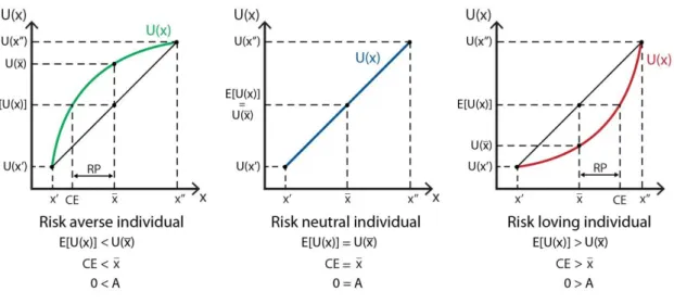
(7) 2. Literature review. 2.1 Risk attitudes and theories of decision One of the most widespread and accepted economic concepts is the pursuit of maximizing expected utility in the decisions of individuals. After years of research, which began in the seventeen century, Daniel Bernoulli was the first who proposed a review of the use of expected value in situations that involved monetary costs and uncertain benefits in his “Exposition of a New Theory on the Measurement of Risk“, 1954, in which he said: “Expected values are computed by multiplying each possible gain by the number of ways in which it can occur, and then dividing the sum of these products by the total number of possible cases where, in this theory, the consideration of cases which are all of the same probability is insisted upon. If this rule be accepted, what remains to be done within the framework of this theory amounts to the enumeration of all alternatives, their breakdown into equiprobable cases and, finally, their insertion into corresponding classifications.” Through this theory, it was John von Neumann and Oskar Morgenstern who, in their book “Theory of Games and Economic Behavior” (1944), developed a more scientific analysis of risk aversion, nowadays known as “Expected Utility Theory”. After this research it can be deduced that if an individual prefers a prospect to its expected value, it is said that the agent is prone to risk and otherwise is said to be risk averse. These notions of risk are linked to the shape of the utility function of the agent: prone attitudes or risk averse, as the utility function of total wealth, i.e., convex or concave, and measured with Arrow Pratt coefficients absolute and relative 1 risk aversion, which measure its concavity or convexity. As it has showed in graphs below, risk aversion (green) may imply that an individual may refuse to play a fair game even though the game’s expected value is zero. However, risk loving individuals (red) may choose to play the same fair game. On the. 1. The coefficient is called relative or absolute as considered or how varies the curvature of the utility function in relation to the level of wealth of the individual.. 7.
(8) other hand, neutral individuals (blue), they are indifferent between playing or not. The utility function for each case can be graphically drawn.2. Figure 1. Risk attitudes as the utility function of total wealth.. Source: policonomics, 2012. Despite the strength of the expected utility theory, it has been found inconsistencies between the implications of expected utility and behavior of the agents at risk, such as the Allais paradox3; for this, it has been emerged alternative theories of expected utility, as the theory of expected utility based on ranges (Quiggin, 1993). This theory is a particular case of The Prospect Theory4 (Tversky and Kahneman, 1979) and it has founded upon two assumptions: the first is based on people process the likelihood of nonlinear mode; and the second one is that individuals pay attention to the results it depends on what relatively good or bad they are. The uncertainty is represented by cumulative distribution functions of probability, and the relations of the prospects preferences are represented by the mathematical expectation of a utility function with 2. RP is the risk premium and A is the Arrow-Pratt measure of absolute risk aversion.. 3. This paradox relies in the fact that in certain types of gambling, although people usually prefer certainty to uncertainty, if they are approached differently, they will prefer the uncertainty that was previously rejected. (Policonomics, 2012) 4. A theory that people value gains and losses differently and, as such, will base decisions on perceived gains rather than perceived losses. Thus, if a person were given two equal choices, one expressed in terms of possible gains and the other in possible losses, people would choose the former. (Investopedia, 2015). 8.
(9) respect to a transformation of the odds on the result set. The probability transform an outcome depends on how preferred (range) is this within the result set. The major advantage that brings the expected utility based on ranges is that, while the expected utility of risk aversion and diminishing marginal utility of wealth are synonymous, under based ranges usefulness are distinguishable and separable concepts. Despite this fact, subsequent researches, for instance, Birnbaum et al. (1999) have proved that in this theory exist some mistakes in mathematics assumptions related to basic principles of expected utility as stochastic dominance, transitivity and various forms of weak independence odds on models based on value ranges. Therefore, empirical work on the subject is not conclusive, and it is a field of study that still open.. As it was anticipated in the introduction, throughout the current studies about attitudes slow to risk, it has concluded, that the demographics are an important factor in the difference in attitudes toward risk. Of these, the most systematically studied has been the gender. One the one hand, Aurora Gallego et. al, (2009) reinforce the notion previously tested by other researchers as Jianakoplos and Bernasek (1998), Powell and Ansic (1997), only just to name a few, about the fact that women are relatively more risk averse than. men. On the other hand, Schubert, Brown, Gysler, and. Brachinger (1999), obtained that "Gender-specific risk propensities arise in abstract gambles, with men being more risk-prone toward gains but women more risk-prone toward losses". 2.2 Measurement of risk aversion According to the previously descripted, there are many possible results in the decision making when the future is uncertain. To measure the degree of risk in an uncertain context, it is necessary to know all the possible results and the probability of these occurring in the future. The most widespread and accepted method by experimentalists when measuring the degree of risk aversion is the one of Holt and Laury (2002) because it has a simple experimental design and also its measures are incentive compatible. In this method, each subject chooses between two lotteries in 10 times. One of these, the least risky, has less variability in payments than the riskiest. In each of the ten times that a decision is taken, the probability of winning the jackpot in lottery is higher. Thus, the 9.
(10) most likely risk players will choose the risky lottery at first, while the others (the least risky) will do it later. In the case of risk neutral subjects, they will choose the risky lottery only when the expected value of each lottery is approximately the same. In the method of Becker et al. (1964) subjects who play a repeatedly set a sale price of a lottery. Given these prices and the parameters of the experiment, it can be estimated a parameter of risk preferences for each subject after playing several rounds. Thus, this method allows accurate estimates. Another method which is easy to implement and allows us to examine the change in utility function curvature for different sets lotteries is the method of Georgantzis and Sabater Grande (2002). It is a variant of Murnigham et al. (1988) and Millner and Pratt (1991). In this, subjects choose four lotteries among two separate groups involving a certain payment odds variables and zero otherwise. Subjects were classified according to their preference lottery choice with a reference probability of 0.5. This method is easy to implement and allows examining the change in curvature for different sets of lotteries.. 2.3 Individuals versus Groups. As has been said before, in economics and finance, most decisions are the result of group discussions, for this reason some researchers focus on finding the differences between the behaviour at individual versus group level in an unknown background. The majority of empirical results based on natural data concerning team versus individual decisions have come from experimental economics. In short, Camerer (2003) concluded his book on Behavioral Game Theory with a section on the top ten research question for future studies “how do teams, groups and firms play games?” Several differences between individual and group decision making have been studied over the past fifteen years in the experimental economics literature. A few of them are presented here. According to Cooper and Kagel (2005) “teams consistently played more strategically than individuals, and their superiority increased with the difficulty of the games. The superior performance of teams is most striking following changes in payoffs that change the equilibrium outcome. Individuals play less strategically following the change in payoffs than inexperienced subjects playing the same game. In contrast, the teams. 10.
(11) exhibit positive learning transfer, playing more strategically following the change than inexperienced subjects.” The fact that groups play more strategically than individuals is reinforced by Alan S. Blinder and John Morgan (2005) through their study, concluding that group decisions are on average, superior and better than individual decisions. However, Sutter (2005) identified several games (with unique equilibrium) where individual decision making entails higher welfare, while in coordination games (with multiple equilibrium), groups achieve more efficient outcomes. In this literature, some economists have studied the differences between groups and individuals considering the risk variable in decision-making. Recent literature has provided that, as a group, people behave in a less risky way, Shupp and Williams (2007). This is due to the relatively less risk averse people are more likely to change their vote in order to adapt to the group; however, those more risk averse behave more rigidly when hanging their preferences. Moreover, there is a positive relationship between preference for risk and willingness to decide alone (David Masclet, Youenn Loheac, et al., 2006).. 2.4 Risk in business. Bowman’s Paradox. As it has been justified above, it can be said that, on the one hand, many of the important decisions arise from the group discussion; an example of it could be how much to invest in a company. On the other hand, it is generally accepted that the risk is an intrinsic part of the financial decisions. For both reasons, it is important to study how the risk affects the business environment. One of the basic assumptions in the world of finance is the positive relationship between return and risk. That is, riskier investments will always be more profitable. Although this statement has been widely contrasted with market measures5, the riskreturn binomial is not true when accounting measures are incorporated; in other words, when it is applied to a business context.. Bowman, in his article published in 1980 was the pioneer in analyzing the risk-return binomial in a business context. In his study, he noted, with a high degree of. 5. The most recent research about this is “Análisis del binomio rentabilidad-riesgo de los activos financieros del IBEX35 para el período 2003-2012” Costa Mosquera, Iván (2013).. 11.
(12) significance and for most sectors of the US, that the relationship between financial performance and its variance is inverse.. From this evidence found by Bowman, it has given rise to a stream of research that lasts until today, trying to explain why this phenomenon. On the one hand, there are scientists who accept the "paradox" and try to give theoretical explanations. Nonetheless, there are those who think that the paradox is the result of statistical errors and deny the existence of it. Among the first, it is important to highlight the studies based on the prospect theory, developed in the early 1980s by the psychologists Daniel Kahneman and Amos Tversky, resulting from the Economy and the theory of the behavior of the company, which come from the Company Organization. Despite their diverse origins, both conclude that, in favorable situations, decision-makers behave as risk averse; however, in unfavorable situations, the urge to get better results will make the subjects become more risk-prone. From this evidence found by Bowman, it has unleashed a stream of research that lasts until today, trying to explain why this phenomenon.. On the other hand, the researchers who deny the paradox, based their studies in two different criteria: many of them question the statistical measures since most jobs defended by paradox supporters use ex-post measurements and this affects the low variance approach that profitability has in relation to the concept of strategic risk. Besides, it is possible that the negative ratio found by Bowman may be result of measuring both variables at any given moment in which they were not in equilibrium and this relationship changes over time. However, to date there has been clarified the nature of the phenomenon, it is a field of research that is still open.. 12.
(13) 3. Methodology and data. The methodology which has been used in this study for data collection and subsequent analysis of the data is commonly used in any study of experimental economics. This section describes in the first part the formalized methodology of experimental economics. In the second and the third section, the hypotheses to be tested in this work as well as the experimental design and data acquisition respectively are shown.. 3.1 Experimental Economics Usually, people have the impression that economists, in their empirical analyzes use databases that are given from the real world for the construction of their variables, as it could be the GDP, exchange rate, interest rate... However, there are other options for obtaining this kind of information, for instance, an experiment. Perhaps, this is not the best option to recruit on a macroeconomic research data, because the experimenter cannot design a controlled situation for all the agents which are involved in this case. Nonetheless, it could be a good method in other areas of the economy such as the Game Theory, which studies the strategic interaction and, it is precisely how subjects interact within controlled strategic environments what allows us to observe an experiment. In these studies, it is possible to create a situation managed by the researcher in an experiment in which some subjects are involved in making decisions that determine how much they will earn trough observing what characteristics influence them. A classic application of experimental economics is to design different market mechanisms in order to know how the different transaction rules lead to more or less efficient results and how the market design variation affects the results. Therefore, this method offers the advantage of controlling the generation of the study variables by the fact that they correspond to real economic situations, although simplified, in which subjects make decisions with consequences for their own pockets through incentives and that all of them are controlled by the experimenter. The economy is distinguished from other social sciences by the importance attributed to the incentives of agents in decision-making. For this reason, in economic experiments, the real incentives are an essential tool for motivating individuals to "tell the truth" and act as similar as possible to the way they would do in a real situation. In 13.
(14) fact, previous researches have proved that monetary incentives are important to consider because it affects in the results of the study, (Barreda-Tarrazona, 2001 and Frey and Jegen, 2001). However others have proved that it is possible getting valid conclusions in the absence of real payments. So, in order to make the incentives of the experiment allow some control over the preferences of individuals, they should be subject to three conditions which are adjusted depending on the type of experiment: 1. Contingency: The amount of incentives received should depend on the decision made by the subject. 2. Dominance: Changes in subject satisfaction with the experiment must be are related basically to changes in incentive amounts received. 3. Monotonicity: A greater incentive payment should always be preferred to a lower payment, and subjects should not get to be filled. Experimental economics has been standardized over the past half century so that today it constitutes a tool of study like econometrics or finance. A justification of this is that it has even its own rewarded with the Nobel Prize in Economics 2002, Vernon Smith, "for having become laboratory experimentation an instrument of empirical economic analysis, especially in the study of different market mechanisms" (experimental economics and game theory, Peter King, February 2006). It is noteworthy that the first game to be tested experimentally was the "Prisoner's Dilemma" (Flood, 1952). Although experimental economics has been the tool used in relevant contributions and it has normalized in recent years as a tool of analysis in the economy, there are still many mistakes in the experimental methodology involving a loss of accuracy in the results. The methodology carried out in this type of analysis and used in the embodiment of the present study must follow a certain order and criteria for obtaining valid results. Here are the steps to follow in conducting an experiment: The first stage of any investigation is the approach to the question of what you want to consider and a justification of what is the appropriate methodology for analysis. This first step in the development of the experiment would be similar to setting the objectives to be achieved after the study. An experiment can fulfill different functions, for example, the study may serve to reinforce some previously tested theory. It could also be the case of several competing hypotheses; in this case, the experiment could help define the range under which each of these hypotheses is valid, thereby 14.
(15) increasing the accuracy of the theory. Finally, it relevant to say that an experiment can have the function of serving as "proof" in the study of new institutions before introducing them to the "real world". An example would be the game led by Ken Binmore, who observed the behavior of subjects under various types of auctions and which was used by the British government to design the auction of licenses for third generation mobile telephony in 2000. Once the experimenter has established the first phase, the second step is to design it. A good experiment can be defined as the one which controls the most plausible hypothesis to explain the phenomenon under study and it should allow the best opportunity to learn something useful as well as answer the question that motivates the research. In this second phase related to the design, all experimentalists must make decisions on at least the following topics: 1. Number of observations: It is necessary to establish the number of observations suitable for subsequent statistical or econometric study, to be established prior to the data collection. The number of observations equals the number of people who have been recruited for the experiment. 2. Payments: As mentioned above, the real monetary incentives are a determining factor in the decision making of individuals. Payments are a way to encourage and motivate the subjects participating in the game, to help them are take the experiment more seriously, and to obtain more conclusive results. The experimentalist must meet the agreed payments while meeting the criteria of contingency, dominance and monotonicity afore mentioned above. It should be considered that it is quite usual to establish a sure payment for the mere fact of participating, this makes the subjects feel satisfied even though the results were not beneficial and encouraged them to participate in further experiments. 3. Instructions: It is possible that many of the subjects participate for the first time in an experiment; it is therefore necessary to establish clear and precise instructions so that all are able to understand, which will also improve post the results. Therefore it is very common that the experimenter reads aloud the instructions before starting the session. Designing a sufficiently clear instructions should prevent questions occur; in case doubts arise, it is best to ask for the answer in public, always avoiding that information other than clarifications of instructions that do it privately and perhaps encourage suspicion 15.
(16) among the subjects to be revealed. It is also important that the instructions provided to the subjects do not lead them to know what is expected from them, as this could skew the validity of the experiment. 5. Repetitions: To set the number of repetitions of the game is a crucial point, because as we know, the most widely accepted interpretation of the concepts of games theory is supposed to be a stable equilibrium which is reached after a learning process (through repetitions). Therefore, it makes sense to study how individuals learn from the experiments and, for this reason, design experiments in which subjects make their decisions repeatedly. 6. Computer: The experimentalist must decide what methods and software will be used, therefore, in these studies, the use of computer terminals enables and streamlines interconnected conducting complicated experiments and collecting data. After the experimental design, the next step is choosing the experimental subjects. Typically, participants in this type of experiments are college students, because normally these studies are conducted in the laboratories of experimental economics in universities. In addition, it is considered that these individuals are more able to understand the concepts and they are a lower opportunity cost since they get satisfied with fewer incentives than other groups of people. Once selected experimental subjects, the fourth phase of this methodology is the experimental session. If it is set a correct design of the experiment, the experimental session should elapse reproduced without errors and under specific conditions. However, although the design is impeccable there may be unforeseen failures such as problems with the informatics service, or the lack of some experimental subjects who agreed to come. Another unexpected that might happen in the session is the lack of monetary resources for making payments; perhaps, the results obtained by subjects may be so good that higher payments should be offered to the individuals even though the experimentalist cannot attend at that time. Anyway, it is assumed that a good experimental design minimizes these problems. At the end of the experimental session, the analyst may already have the data to analyze them. It is important at this point to realize that the data recording includes not only the variables representing the decisions of individuals, but also the conditions in which these variables were collected: the different treatments that may exist, the order in which decisions have been taken... etc. Note that a particularly complex quantitative 16.
(17) analysis is not needed to obtain a valid and compelling analysis of the data. In fact, if all the methodological procedure has been in the best way possible, a basic statistical analysis should allow us to test our hypotheses. Finally, the last phase of experimental methodological procedure is that the analyst decides which obtained results will be published. Although selecting only some of the conclusions obtained, it is necessary to provide everything that has led to the results, so that another experimenter could be able to reproduce the same study (forms of instruction, obtained original data, recruitment procedures subject ...) It should be mentioned that at present, since 1998 there is a specific journal for publication of experimental items, Experimental Economics.. 3.2. Hypothesis Based on the literature described in the section 2 about previous research on the topic of this paper, we have established three hypotheses to be tested in this study:. H1: Women are more averse than men in the taking of individual decisions. However, in group decision making there is not a significant different between the decisions of groups formed by a majority of women and those with a majority of men.. Building on previous studies, particularly the research of Aurora Gallego et. al. (2009), through this hypothesis it is intended to reinforce the idea that there are significant differences in the level of risk in making individual decisions between male and female. Additionally, it aims to provide, through the comparison of results of individual and group elections, that the relevance of the gender variable in making individual decisions is not as relevant in making group decisions. Although there are no studies proving that the gender variable is not relevant in making group decisions, the reason that has led to raise it is the following: in group decision making come into play much more social factors and personality characteristics which are necessary take into account, for instance vulnerability (Shupp and Williams, 2003) which could cause the effect of gender is not as significant as individual decision making.. 17.
(18) H2: In the context of decision making in repeated business task, groups become relatively riskier over time.. According to Shupp and Williams (2003), it has proved that, as a group, people behave less risky way. This is due to the relatively less risk averse people are more likely to change their vote in order to adapt to the group. However, there is no empirical evidence. about. how. this. change. in. behavior. evolves. over. time.. In the first period, it might be logical that these individuals, in order to adapt to the group, they change their vote and consequently, groups choose less risky strategies; but in subsequent periods, because of the confidence in the group increases, these subjects are not as vulnerable as the beginning and they start behaving like themselves. Consequently, in more advanced periods, the risk level of the strategies increases.. H3: In a business task, groups who have opted for riskier strategies have earned higher profits.. As has been mentioned in Part 2 it has not already reached a consistent theory to show that the risk-return is true in the business area. After analyzing this hypothesis it has pretended to test whether Bowman paradox is true in this experimental design.. 3.3 Experimental design and data As explained at the beginning of the section, the data collection for this study has been through an experiment conducted by Iván Barreda Tarrazona and Alma Rodríguez Sánchez held at the Laboratory of Experimental Economics at the UJI. This aimed at learning about the functioning of the working groups in two contexts: the creative which will not be considered in the present work- and in a context of uncertainty -on which this study focuses through the analysis of various tasks- (business game and risk lottery).. 18.
(19) Business Task The number of subjects in the experiment, and therefore the number of observations, is 286 people, (185 women and 101 men) who form 41 groups compounds from 4 to 6 people in the case of risk task. They have different ages (from 18 to 67) and different professions. (business. students,. psychology. students,. nurses,. housewives,. unemployed people…) This task consisted of a business simulator, through which subjects (grouped in no particular pattern) took decisions as directors managers aiming to get as many possible benefits or higher cash. The company in question was engaged in selling last generation mobile phones, a growing market characterized by its high level of competence. The experiment was conducted in three sessions6, three different days. In each of the sessions it started from zero, i.e., the benefits of the first treatment did not influence on the results of the second and third. In addition, at each meeting at least three decisions were made and all of them should have taken into account these aspects: production, sale price and acquisition of raw materials. These decisions amounted to a real working week and users should consider that some of the decisions they took did not have immediate effects, but long term. Regarding the information available from the subjects, they only knew the information about decisions taken by the former managers (week -1). In addition to this information, which was provided for free, they had an additional: if they paid 500UMEs they could buy reports on how their company was developing. In any case, the subjects could have external information about the decisions of the other groups and their results, a factor which, as will be seen below, had effects on the results obtained in this study (part 7). To measure the level of risk assumed in every decision by each groups the business decisions have been analyzed by an individual independent expert. The following is a summary table on the classification of the strategies according to their risk level shown in ascending order. That is, from the most conservative strategy (1, shark strategy), which is based on trying to get profit from the sale of what is already available to the company, without pursuing more ambitious objectives; the riskier (5), which pursues. 6. From here, along the paper, the three sessions, will be named as three treatments.. 19.
(20) the expansion and differentiation with significant investments assuming, therefore, greater risks. Risk level 1 Shark strategy: to dismantle the company, low-risk strategy. 2 Conservative strategy: keep everything the same or minor changes. 3.1 Expansive strategy: increase production, increase purchases, maintain or reduce prices. 3.2 Differentiation strategy: the price increase, maintain or reduce production and increase advertising. 4 Expansive and differentiation strategy (simultaneous dual strategy): increase production, more raw materials maintain or decrease prices and increase advertising. 5 Aggressive strategy: expansion and / or differentiation with significant investments (purchase of machinery, hiring, higher advertising expenses ...). 0 Inconsistent Strategy: conflicting decisions doomed to failure.. Lotteries task At the end of each of the three treatments users participated in the lottery task, wholly independent from the one described above. In it, participated users themselves but in this case, the same participants but individually and they could earn an amount of money depending on the decisions they took. Each lottery had 4 panels. The task of the subjects was to choose one of the 10 alternatives of each panel. Each alternative is a lottery defined as a combination of the probability of winning and the amount (in €) if they could get out the favorable result. If the outcome was not favorable, they did not win anything. Therefore, these were the steps7: 1. Choose an alternate from each of the 4 panels. 2. The experimenter threw a 4-sided die. The number left (1, 2, 3 or 4) determined the panel with which the user was playing in the next step.. 7. The instructions have been extracted from the experimenter notebook. .. 20.
(21) 3. The experimenter threw a 10-sided die (from 0-9). The number indicated the number went from which the prize is not won. That is, if it is marked on the panel e.g. choosing 5 (probability 0.5) the given number 5 to get the number 5, will win the prize that corresponds to that option, and also all those who have scored less options (0, 1, 2, 3 and 4). Those who have scored top choices (6, 7, 8 and 9) will gain nothing. But if it has marked number 5 (probability 0.5) and given out at 0, 1, 2, 3 or 4 nothing would be gained. There is the possibility of getting always win if the number 0 in all panels is checked, but the gain will be much smaller, only 1 €. Session 1 was a test session, so the result is favorable although no money is received. However, in sessions 2 and 3 it was paid in cash based on money earned. Then, it is shown the lotteries used in the experiment designed by Sabater-Grande and Georgantzis, 2002. Panel 1 Dado. 0. 1. 2. 3. 4. 5. 6. 7. 8. 9. Prob.. 1. 0,9. 0,8. 0,7. 0,6. 0,5. 0,4. 0,3. 0,2. 0,1. €. 1,00 1,10 1,30 1,50 1,70 2,10 2,70 3,60 5,40 10,90. Elección. Panel 2 Dado. 0. 1. 2. 3. 4. 5. 6. 7. 8. 9. Prob.. 1. 0,9. 0,8. 0,7. 0,6. 0,5. 0,4. 0,3. 0,2. 0,1. €. 1,00 1,20 1,50 1,90 2,30 3,00 4,00 5,70 9,00 19,00. Elección. Panel 3 Dado. 0. 1. 2. 3. 4. 5. 6. 7. 8. 9. Prob.. 1. 0,9. 0,8. 0,7. 0,6. 0,5. 0,4. 0,3. 0,2. 0,1. €. 1,00 1,70 2,50 3,60 5,00 7,00 10,00 15,00 25,00 55,00. Elección. 21.
(22) Panel 4 Dado. 0. 1. 2. 3. 4. 5. 6. 7. 8. 9. Prob.. 1. 0,9. 0,8. 0,7. 0,6. 0,5. 0,4. 0,3. 0,2. 0,1. €. 1,00 2,20 3,80 5,70 8,30 12,00 17,50 26,70 45,00 100,00. Elección. After the experiment described above, the data (group and individual) were collected to create the different variables under statistical analysis in this paper, through the SPSS program.. Group data The variables considered in the analysis of the groups are the risk level strategies (strategy_T1,. strategy_T2,. strategy_T3),. profits. (accumulated_profit_T1,. accumulated_profit_T2, accumulated_profit_T3) and proportion of women in each group (proportion_women) The variables about strategy refer to the level of risk present in the same (in ascending order), as it has explained in TABLE 1. These variables are constructed from the data that have been collected from the business task described above. It is necessary to further explain that the strategies that have been labeled with 0, could not be classified according to the level of risk, they are inconsistent and contradictory. Therefore, data relating to the groups that have followed such strategies have been eliminated from the study, since its inconsistency could hinder the subsequent statistical analysis. They are a total of 9 groups. Therefore, the variables strategy_T1, strategy_T2, strategy_T3, now only take the values 1-5. In the case of profits variables, they show the accumulated profits that groups have obtained in three periods respectively. On the other hand, the variable “proportion_women” has been constructed in order to compare more tightly the differences in risk aversion between men and women in individual and group decision making (through correlation analysis). For the analysis of group decisions it has been necessary to create a base of aggregated data in which an observation per group was collected (each group, regardless of the number of people for which it is constituted, takes a joint decision).. 22.
(23) Individual data In this case, the variables have been built through the individual data from lotteries. The variables considered in the analysis of the individuals are GENDER, LOT_PANEL1, LOT_PANEL2, LOT_PANEL3, LOT_PANEL4. As for the gender variable has been treated as a dummy variable that takes value 1 if the subject is female and 0 if it is a man. In the case of variables LOT_PANEL1, LOT_PANEL2, LOT_PANEL3, LOT_PANEL4 the values taken (from 0-9) are interpreted as the level of risk taken in each election, in ascending order; that is, an individual who chooses an option panel 9 shows a greater prone for risk or lower risk aversion than who chooses option 0 (secure payment) As in the treatment of group data, it has been chosen for the elimination of number of samples by the lack of data since some subjects lacked any of the three sessions, namely, 4. To follow the same approach in the treatment of data, the individuals with missing data in the risk task have forced to remove these observations in this group data base too because it is useless to analyze the differences observed in both contexts if subjects participating in them are not the same. (If a person missing data, it have been removed from the sample to all individuals in the group). After removing necessary data, the new sample is composed by 201 (135 women and 66 men) people and 41 groups. This reduced database is to be used for subsequent analysis.. 23.
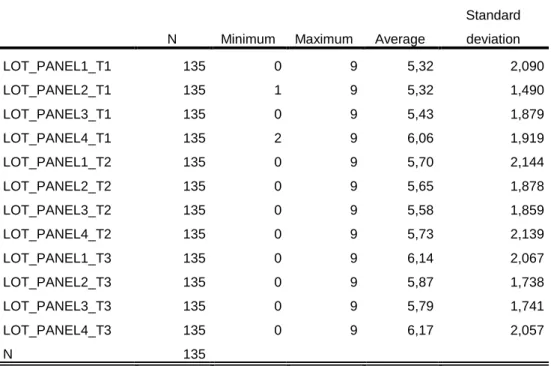
(24) 4. Results and discussion. In this section it is shown the results obtained by analyzing data in SPSS Statistics program, based on the assumptions described in the previous section. Result 1: Men are less risk averse than women in making individual decisions. However, in group decision making, gender variable is not as relevant in the risk level of the decisions. In the tables below (TABLE 1 and TABLE 2), it is shown a comparison of the descriptive statistics (mean, standard deviation, minimum and maximum) for the variables: LOT_PANEL1, LOT_PANEL2, LOT_PANEL3, LOT_PANEL4 in the three treatments between women and men, respectively. As shown, the value of the average for men is higher in all cases studied. The fact that these values are higher, on average, in the case of men, means that, in general, male have opted for riskier decisions on all panels of lotteries, consequently, women show a greater aversion risk. This result is consistent with the research of Aurora Gallego et. al. (2009) mentioned previously.. Table 1. Descriptive statistics. Lottery choicesa Standard N. Minimum. Maximum. Average. deviation. LOT_PANEL1_T1. 135. 0. 9. 5,32. 2,090. LOT_PANEL2_T1. 135. 1. 9. 5,32. 1,490. LOT_PANEL3_T1. 135. 0. 9. 5,43. 1,879. LOT_PANEL4_T1. 135. 2. 9. 6,06. 1,919. LOT_PANEL1_T2. 135. 0. 9. 5,70. 2,144. LOT_PANEL2_T2. 135. 0. 9. 5,65. 1,878. LOT_PANEL3_T2. 135. 0. 9. 5,58. 1,859. LOT_PANEL4_T2. 135. 0. 9. 5,73. 2,139. LOT_PANEL1_T3. 135. 0. 9. 6,14. 2,067. LOT_PANEL2_T3. 135. 0. 9. 5,87. 1,738. LOT_PANEL3_T3. 135. 0. 9. 5,79. 1,741. LOT_PANEL4_T3. 135. 0. 9. 6,17. 2,057. N. 135. a. Gender = female. 24.
(25) Table 2. Descriptive statistics, Lottery choicesa Standard N. Minimum. Maximum. Average. deviation. LOT_PANEL1_T1. 66. 0. 9. 5,80. 2,248. LOT_PANEL2_T1. 66. 2. 9. 5,64. 1,585. LOT_PANEL3_T1. 66. 1. 9. 5,92. 1,658. LOT_PANEL4_T1. 66. 2. 9. 6,26. 1,900. LOT_PANEL1_T2. 66. 0. 9. 6,59. 2,148. LOT_PANEL2_T2. 66. 3. 9. 6,58. 1,737. LOT_PANEL3_T2. 66. 3. 9. 5,89. 1,609. LOT_PANEL4_T2. 66. 3. 9. 6,36. 1,943. LOT_PANEL1_T3. 66. 2. 9. 6,88. 1,810. LOT_PANEL2_T3. 66. 3. 9. 6,53. 1,629. LOT_PANEL3_T3. 66. 2. 9. 6,09. 1,829. LOT_PANEL4_T3. 66. 3. 9. 6,48. 1,685. N válido (por lista). 66. a. Gender = male. After this comparison, these results have been tested by Mann-Whitney U test, a nonparametric test applied to two independent samples, in order to determine whether these differences in descriptive statistics are relevant. Thus, the hypothesis to be studied is:. H0: The medians of both groups are equal (no significant differences in risk aversion between men and women). H1: The medians of both groups are different (null hypothesis is not true, there are differences). Through the analysis of the test, it can be stated, for the first treatment, that these differences in the distribution are not significant in any of the four panels. However, for the treatment two and three, there are significant differences in the median between men and women; particularly in the first two panels. Then, in tables 3 and 4 it is shown the summary tables of hypothesis tested that have been obtained.. 25.
(26) Table 3. Abstract hypothesis contrast. Treatment 1. Null hypothesis. Test. Sig.. Decission. 1. LOT_PANEL1_T1 medians are the same between gender categories. Mann-Whitney U test for independent samples. ,426. Keep the null hypothesis.. 2. LOT_PANEL2_T1 medians are the same between gender categories. Mann-Whitney U test for independent samples. ,431. Keep the null hypothesis.. 3. LOT_PANEL3_T1 medians are the same between gender categories. Mann-Whitney U test for independent samples. ,710. Keep the null hypothesis.. 4. LOT_PANEL4_T1 medians are the same between gender categories. Mann-Whitney U test for independent samples. ,673. Keep the null hypothesis. Asymptotic meanings are found. The significance level is 05.. The fact that for all panels of period 1 the differences between the choices of men and women are not significant, it may be because, as it has been explained in the experimental design, unlike periods 2 and 3, in the first, the payments were hypothetical. When payments are not real, it is possible that more risk averse people (in this case, men), change their attitude. This first result is consistent with previous studies of Barreda-Tarrazona (2001) and Frey and Jegen (2001), who proved that monetary incentives are important to consider because it affects in the results. However, this result differs from Jamal et al. (1991), and Melo (1993) studies, who proved valid conclusions in the absence of real payments. Noting the results for the first period, we will analyze together the following two. The summary of the assumptions for these periods are shown below.. 26.
(27) Table 4. Abstract hypothesis contrast. Treatments 2 and 3. Null hypothesis. Test. Sig.. Decision. 1. LOT_PANEL1_T2 medians are the same between gender categories. Mann-Whitney U test for independent samples. ,003. Reject the null hypothesis.. 2. LOT_PANEL2_T2 medians are the same between gender categories. Mann-Whitney U test for independent samples. ,001. Reject the null hypothesis.. 3. LOT_PANEL3_T2 medians are the same between gender categories. Mann-Whitney U test for independent samples. ,359. Keep the null hypothesis.. 4. LOT_PANEL4_T2 medians are the same between gender categories. Mann-Whitney U test for independent samples. ,056. Keep the null hypothesis. 1. LOT_PANEL1_T3 medians are the same between gender categories. Mann-Whitney U test for independent samples. ,050. Keep the null hypothesis. 2. LOT_PANEL2_T3 medians are the same between gender categories. Mann-Whitney U test for independent samples. ,021. Reject the null hypothesis.. 3. LOT_PANEL3_T3 medians are the same between gender categories. Mann-Whitney U test for independent samples. ,632. Keep the null hypothesis.. 4. LOT_PANEL4_T3 medians are the same between gender categories. Mann-Whitney U test for independent samples. ,852. Keep the null hypothesis. Asymptotic meanings are found. The significance level is 05.. 27.
(28) As can be seen, in treatment 2, the null hypothesis (no significant differences in risk aversion between men and women), is rejected; therefore, to a level of significance of 5% it can say that women are more risk averse than men in the first two panels of treatment 1. In treatment 3 the result is almost the same; although in this case, in the panel 1 it is not possible to reject the null hypothesis (U coefficient = significative level = 0.05). One possible reason for this difference between the significance of the first two panels and the two seconds could be the difference in payments. As it is shown in lotteries, in each panel, payment was increased, therefore, it could be concluded within the same result, that higher payments, minor differences in risk behavior between men and women; with increases of the expected payoff, women become less risk averse. Here ends the analysis at the individual level, and then it is shown the analysis of the data groups used to compare both contexts.. Table 5. Correlations between the proportion of women in groups and the risk level of the strategies.. Rho de Spearman. N. Proportion_women and Strategy_T1. -,074. 41. Proportion_women and Strategy_T2. -,030. 41. Proportion_women and Strategy_T3. ,419**. 41. T1. T2. T3. **. Correlation is significant at the 0.01 level. Table show that for the first two treatments, there is a negative correlation between the percentage of women in the group and the level of risk strategies. That is, the groups with majority of women are more risk averse. But this correlation is not significant; 28.
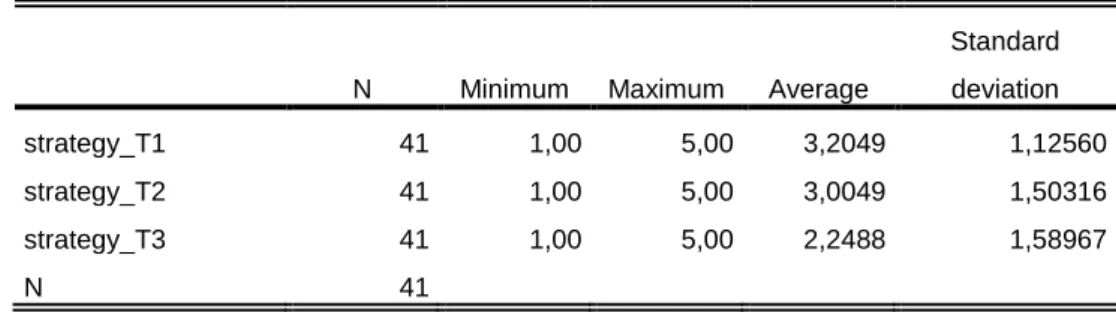
(29) however, in treatment 3, the correlation is positive and significant at 1%. The groups with the highest percentage of women are taking more risky strategies.. If we compare the results we have obtained in both analyses (individual and group), we can conclude that: Women are more risk averse in making individual decisions, however, this theory is not valid in making group decisions.. Result 2: The level of risk in the strategies implemented by the groups decreases in time. After analyzing the descriptive statistics of the variables strategy3 strategy2 strategy1, which collect the level of risk of decisions in the three periods studied, respectively, it can be said that, on average, the level of risk decreases in each period. Thus, we find that the hypothesis 2 arisen in the previous part is not true; it has not obtained the expected result. Instead, the results obtained through the descriptive statistics shown in Table 5 indicate otherwise. This evolution of the level of risk of the strategies decreases along the three periods.. Table 6. Descriptive statistics. Risk level of the strategies. Standard N. Minimum. Maximum. Average. deviation. strategy_T1. 41. 1,00. 5,00. 3,2049. 1,12560. strategy_T2. 41. 1,00. 5,00. 3,0049. 1,50316. strategy_T3. 41. 1,00. 5,00. 2,2488. 1,58967. N. 41. Then, it is showed firstly, the frequency histograms about the risk level of strategies adopted by groups in each of the three treatments. Secondly, the same information but now separated by gender (groups with majority of women vs. groups with majority of men).. 29.
(30) Figures 2-10. Frequency histograms. Risk level of strategies.. Strategy_T1. frequency. Average = 3.20 Standard derivation = 1.126 N = 41. Strategy_T1. Strategy_T2 frequency. Average = 3 Standard derivation = 1.503 N = 41. Strategy_T2. Strategy_T3 frequency. Average = 2.25 Standard derivation = 1.59 N = 41. Strategy_T3 Strategy_T3. 30.
(31) a.. Groups with majority of women. Strategy_T1. Strategy_T2. Strategy_T3. b. Groups with majority of men. Strategy_T1. Strategy_T2. Strategy_T3. 31.
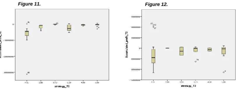
(32) According to Shupp and Williams (2003), more risk-loving individuals are more vulnerable when it comes to change the choices to riskier strategies. In the hypothesis 2 it has presented that in the first period, those subjects less risk averse change their vote and consequently, groups choose less risky strategies; but in subsequent treatments, because of the confidence in the group increases, these subjects are not as vulnerable as the beginning and they start behaving like themselves. Consequently, in more advanced periods, the risk level of the strategies increases. In this case, the fact that the risk level of the strategies, in general, decreases in time it could be because, over time, instead of behaving as they themselves, they become more vulnerable and consequently, less risky strategies dominate. However, if we compare the groups with majority of women and groups with majority of men we note that in the treatment 3, groups with majority of men have reduced much more the level of risk in their strategies. This result justifies the above. The fact that in general, in treatment 3, there are a positive correlation between the proportion of women in the group and the level of risk is because, although all groups are decreasing the risk level of the strategies, the groups with majority of men are doing relatively more, i.e., women are behaving relatively more risk prone.. Result 3: Groups that have opted for riskier strategies have earned higher profits.. The tables below present the correlations between the level of risk of the strategies chosen by the groups and the accrued benefit derived from them.. Table 7. Correlations between the risk level of strategies and accumulated profit.. Rho de Spearman. N. Strategy_T1 and ccumulated_profit_T1. -,048. 41. Strategy_T2 and ccumulated_profit_T2. ,508**. 41. Strategy_T3 and ccumulated_profit_T3. ,289*. 41. T1. T2. T3. **. Correlation is significant at the 0.01 level. *. Correlation is significant at the 0.05 level. 32.
(33) After analyzing the Spearman coefficient, a significant positive correlation is obtained in treatment 2 and 3; thus, the result can be interpreted as follows: groups with more risky strategies, earn higher benefits. This result may appear inconsistent with the previous one since it makes no sense that the groups take less risky strategies along the time if greater benefit is obtained assuming greater risks. A justification for this could be that the subjects do not know the strategies of their rivals and the results they are getting, therefore, unaware that they are risking more groups are getting more profits and consequently, do not opt for increasingly risky strategies.. In the following boxplot figures, it can be seen that this correlation is more significant between 1 and 2 strategy (less risky). That is, there are important differences in profits in terms of these two strategies (Strategy 2 provides a greater profit than strategy 1); however, in riskier strategies, the increased in profits is not observable. The fact that higher risk entails higher profits is consistent with one of the basic principles of the financial environment, the risk-return binomial. However, this result differs from the study of the paradox of Bowman, who, as mentioned in part 2, he stated that the risk-return stop fulfilled in business when accounting standards were taken into account.. Figure 11.. Figure 12.. For a better analysis, we have differentiated the cumulative profit for groups with majority of men and the groups with majority of women. As we can see, if we analyze the histograms, we observe that this result is consistent with the two above. Groups with majority of women are obtaining higher benefits than the groups with majority of men, because they assume relatively greater risks in time. 33.
(34) Figures 13-18. Frequency histograms. Accumulated profits. b.. Groups with majority of women. Accumulated_profit_T1. Accumulated_profit_T2. a.. Groups with majority of men. Accumulated_profit_T1. Accumulated_profit_T2. 34 Accumulated_profit_T3. Accumulated_profit_T3.
(35) Result 4: In treatment 3, groups with majority of women become more risk prone after the bad experience in the first two periods. In other words, toward losses, women are more risk prone than men. First of all, for result 1, we had observed a striking change in treatment 3. In first 2 treatments, the correlation between the proportion of women in the group and the level of risk was negative. However, in treatment 3 this correlation was positive and significative (at 1%). Then, we have obtained that in time, groups in general, behaved like more risk averse but in particular, groups with majority of men, in treatment 3, were behaved relatively more risk averse than groups with majority of women. For last, in result 3, the analysis showed that riskier groups obtained higher profits, in this case, groups with majority of women. All these previous results lead us further. Although in the experiment, they did not know the results of their opponents at the end of each period, they know their own. As we have seen in the histograms of accumulated profits, the results obtained in earlier periods are very unfavorable. After this fact, depends on gender, subject have reacted in different ways. On the one hand, toward losses, women become riskier prone; however, men became more risk averse. Thus, in treatment 3 we can observe it: groups with majority of men reduce relatively much more the risk of their strategies than groups with majority of women. This result is compatible with the previous research of Schubert, Brown, Gysler, & Brachinger (1999), who obtained that "Gender-specific risk propensities arise in abstract gambles, with men being more risk-prone toward gains but women more riskprone toward losses". 35.
(36) 5. Conclusions. After the empirical analysis carried out in this work, we have demonstrated that through an experimental methodology are possible obtaining valid results. We have achieved the objectives proposed in first lines of this paper which were to strengthen that gender is an important variable in the decision making under uncertainty as well as to know how risk attitudes affect the results of a company.. A basic statistical analysis has been enough to test the three hypotheses considered. Through the two tasks realized in the experiment (lotteries and task) it has been possible to recollect and create the necessaries variables to analyze our starting assumptions and achieve four results. First of all, in result 1 we have reinforced the previous theory generally accepted about women behave more risk averse than men in individual decision making (lottery task); however, this theory is not true in group decision making (business task) where we have obtain, for treatment 3, that groups with majority of women have become more risk prone. Secondly, though the result 2 we can say that the risk level of the strategies implemented by the groups, in general, decreases in time. Within this result, there is an evidence that, in particular, groups with majority of men have become relatively more risk averse than groups with majority of women. Thirdly, it has obtained that groups that have opted for riskier strategies have earned higher profits (groups with majority of women have obtained higher profits since they have opted by riskier strategies). Lastly, three previous results have led us to assert that toward losses, women are more risk prone than men. In general, in three treatments profits have been unfavorable; thus, in last treatment, noting these losses, groups with majority of women opt for risking relatively more. However, with losses, groups with majority of men have become relatively more risk averse.. Throughout the study we found some limitations that have been difficult to obtain more precise results. The fact that in the experiment each group took a different number of decisions implies that they are not under the same conditions and this can lead to errors in the results. Another limitation that we have obtained is related to the classification of strategies. If strategies had been evaluated by a group of people, instead of only one person, perhaps it would have averted more subjectivities, and they would be more accurate.. 36.
(37) For future related studies, it would be advisable to extend the sessions of the experiment, in order to obtain more precise results about the evolution of the risk level of the strategies in time. It is possible that some groups have opted for long-term strategies and they have not enough time to see the result of the same. Perhaps for this reason many of the strategies have been inconsistent and it has been necessary to remove part of the sample.. 37.
(38) References. -Ansic, D. and Keasey, K. (1994). Repeated decisions and attitudes to risk. Economics Letters, 45(2), pp.185-189. -Barreda-Tarrazona, I., Jaramillo-Gutiérrez, A., Navarro-Martínez, D. and SabaterGrande, G. (2011). Risk attitude elicitation using a multi-lottery choice task: Real vs . hypothetical incentives. Spanish Journal of Finance and Accounting / Revista Española de Financiación y Contabilidad, 40(152), pp.613-628. -Bernoulli, D. (1954). Exposition of a New Theory on the Measurement of Risk. Econometrica, 22(1), p.23. -Blinder, A. and Morgan, J. (2005). Are Two Heads Better Than One? Monetary Policy by Committee. Journal of Money, Credit, and Banking, 37(5), pp.798-811. -Camerer, C. (2003). Behavioral game theory. New York, N.Y.: Russell Sage Foundation. -Cooper, D. and Kagel, J. (2005). Are Two Heads Better Than One? Team versus Individual Play in Signaling Games. American Economic Review, 95(3), pp.477509. -Gallego, L. (2015). Policonomics, economics made simple. [online] Policonomics.com. Available at: http://www.policonomics.com/ [Accessed 10 May 2015]. -García-Gallego, A., Georgantzís, N. and Jaramillo-Gutiérrez, A. (2008). Ultimatum salary bargaining with real effort. Economics Letters, 98(1), pp.78-83. -Holt, C. and Laury, S. (2002). Risk Aversion and Incentive Effects. American Economic Review, 92(5), pp.1644-1655. -Jianakoplos, N. and Bernasek, A. (1998). are women more risk averse?. Economic Inquiry, 36(4), pp.620-630. -Kahneman, D. and Tversky, A. (1979). Prospect Theory: An Analysis of Decision under Risk. Econometrica, 47(2), p.263. -Laury, S. and Holt, C. (n.d.). Further Reflections on Prospect Theory. SSRN Journal. -Masclet, D., Colombier, N., Denant-Boemont, L. and Lohéac, Y. (2009). Group and 38.
(39) individual risk preferences: A lottery-choice experiment with self-employed and salaried workers. Journal of Economic Behavior & Organization, 70(3), pp.470484. -Millner, E. and Pratt, M. (1991). Risk aversion and rent-seeking: An extension and some experimental evidence. Public Choice, 69(1), pp.81-92. -Millner, E., Pratt, M. and Reilly, R. (1988). A re-examination of Harrison's experimental test for risk aversion. Economics Letters, 27(4), pp.317-319. -Núñez,. M.. (2000).. [online]. E-archivo.uc3m.es.. Available. at:. http://e-. archivo.uc3m.es/bitstream/handle/10016/13850/paradoja_nuneznickel_AECA_2000.pdf?sequence=1 [Accessed 27 Jun. 2015]. -Powell, M. and Ansic, D. (1997). Gender differences in risk behaviour in financial decision-making: An experimental analysis. Journal of Economic Psychology, 18(6), pp.605-628. -Quiggin, J. (1993). Testing between alternative models of choice under certaintycomment. Insurance: Mathematics and Economics, 13(2), pp.160-161. -Rey, P. (2006). [online] Available at: http://pareto.uab.es/prey/EEyTJ.pdf [Accessed 27 Jun. 2015]. -Sabater-Grande, G. and Georgantzis, N. (2002). Accounting for risk aversion in repeated prisoners’ dilemma games: an experimental test. Journal of Economic Behavior & Organization, 48(1), pp.37-50. -Schubert, R., Brown, M., Gysler, M. and Brachinger, H. (1999). Financial DecisionMaking: Are Women Really More Risk Averse?. American Economic Review, 89(2), pp.381-385. -Shupp, R. and Williams, A. (2007). Risk preference differentials of small groups and individuals*. The Economic Journal, 118(525), pp.258-283. -Von Neumann, J. and Morgenstern, O. (1953). Theory of games and economic behavior. Princeton: Princeton University Press.. 39.
(40)
Figure

+2
Documento similar