Approach to Area Coverage and Path Planning for Fleets
of Mini Aerial Robots
• • • • • • • • • • • • • • • • • • • • • • • • • • • • • • • • • • • •
Antonio Barrientos, Julian Colorado, and Jaime del Cerro Centre for Automation and Robotics, UPM-CSIC, Madrid, Spain Alexander Martinez
Centre for Automation and Robotics, UPM-CSIC, Madrid, Spain, and Robotics and Automation Group, Pontificia Universidad Javeriana, Cali, Colombia
Claudio Rossi, David Sanz, and Jo ˜ao Valente
Centre for Automation and Robotics, UPM-CSIC, Madrid, Spain e-mail: [email protected]
Received 9 December 2010; accepted 11 June 2011
In this paper, a system that allows applying precision agriculture techniques is described. The application is based on the deployment of a team of unmanned aerial vehicles that are able to take georeferenced pictures in order to create a full map by applying mosaicking procedures for postprocessing. The main contribution of this work is practical experimentation with an integrated tool. Contributions in different fields are also reported. Among them is a new one-phase automatic task partitioning manager, which is based on negotiation among the aerial vehicles, considering their state and capabilities. Once the individual tasks are assigned, an optimal path planning algorithm is in charge of determining the best path for each vehicle to follow. Also, a robust flight control based on the use of a control law that improves the maneuverability of the quadrotors has been designed. A set of field tests was performed in order to analyze all the capabilities of the system, from task negotiations to final performance. These experiments also allowed testing control robustness under different weather conditions.C 2011 Wiley Periodicals, Inc.
1. INTRODUCTION
The concept of precision agriculture (PA) has emerged in re-cent years as a farming management strategy. Several defi-nitions have been proposed (Srinivasan, 2006). In brief, the concept of PA is to use information technologies to collect and process data from multiple sources for improving the understanding and management of soil and landscape re-sources in order to handle crops in a more efficient way. It allows not only assisting farmers to take decisions but also automating some basic farming tasks. Automation applied to agricultural tasks is still in an early stage, mainly due to difficult working conditions, such as irregular terrains, dif-ferent soils, unstructured environment, and harsh environ-mental conditions (temperature, rain, humidity, dust, etc.). Remote sensing (RS) techniques are basic components of PA. One of the most often applied RS techniques is aerial imagery, but its main weakness is limited availability in the narrow time windows for the images to be obtained. In fact, farmers are interested in recollecting and analyzing data of particular growth stages that can last as short as a few days.
A multimedia file may be found in the online version of this article.
Currently, there are three main ways for obtaining aerial images: satellites, planes, and unmanned aerial ve-hicles (UAVs). Using satellite images has an extremely high cost for small farmers and has very low availability, mainly due to the small number of satellites and the dependency on the weather when it covers the area of interest. For these reasons, satellite images become unpractical. Until recently, commercial flights have been the most feasible way for ob-taining aerial images; nevertheless they are still very costly and have low availability due to the small number of com-panies dedicated to this activity. Moreover, they are highly dependent on the weather.
The reduction in the cost of high-precision GPS re-ceivers and the development of small integrated inertial sensors have boosted the creation of the several companies dedicated to developing small UAVs. Initially, UAVs were based on helicopters, but most of them are now based on quadrotors, because they have a more simple mechanics and therefore are more robust.
Aerial imagery is mainly employed in field obser-vation and map generation by using images that con-tain information about the biophysical parameters of the crop field (Burgos-Artizzu, Ribeiro, Tellaeche, Pajares, & Fern´andez-Quintanilla, 2010; Curran, 1985). Two typical
applications are weed detection with high-resolution re-quirements and hydric stress determination using lower resolution.
Typically, maps are built by stitching a set of georef-erenced images through mosaicking procedures. The high-precision positioning of the UAVs and the capability of performing hovering while delivering high-resolution cam-eras (i.e., color or multispectral camcam-eras) make them the most suitable choice for performing mosaics. Neverthe-less, the most relevant drawback of this solution is the limited autonomy of the mini aerial vehicles. This limita-tion bounds the area that can be covered by an individual robot. Consequently, in order to cope with the typical size of crop fields, either multiple flights or a group of robots is required.
In this paper, a feasible solution for performing aerial imaging applied to PA by using a fleet of UAVs is pre-sented. This paper provides a unified view of the modules and the field work that we have been carrying out in mul-tirobot task planning, path planning, and UAV control.
1.1. The Approach Proposed and Paper Outline
The system provides a decoupled solution, because the methodology employed can be easily divided into two steps. Figure 1 is the global system flowchart. Initially, the target workspace is defined in the crop field by using geo-referenced points. It is subsequently provided to the area-partitioning step. The resulting subareas are discretized ac-cording to the required spatial resolution. Path planning is then executed for each subarea. Finally, individual flight plans are sent to the quadrotors in order to be performed. The main issues of the proposed solution are as follows:
• Task subdivision and allocation. This is a classical problem in multirobot coordination. Given a global task
T0andRrobots, the problem is how to partitionT0into
Rnonoverlapping subtasks and how to assign subtasks
to the robots for their execution. As a contribution of this
work, the proposed tool simultaneously provides solu-tions for the two mentioned problems in a distributed way applied to UAV restrictions: each robot is aware of its own characteristics and status but does not know anything about those of its teammates. In this approach,
the original taskT0is the area to be surveyed, which is
divided into subareas through a negotiation process in which each robot claims covering as much area as possi-ble. This solution is reviewed more deeply in Section 2.
• Path planning. Once the subareas are assigned, each robot is in charge of accomplishing its covering mission by following a path. This path typically consists of a set of waypoints that have to be computed. A waypoint is a position where a sample (i.e., an image) has to be taken. To solve this problem, coverage path planning (CPP) techniques are used. CPP is a subfield of motion plan-ning that addresses the problem of determiplan-ning the com-plete coverage path for a robot in the free workspace. CPP algorithms for UAVs are few. In this work, a prac-tical implementation was successfully carried out. The path planning issue is studied in detail in Section 3.
• Aerial vehicles’ control.Although accuracy in control-ling the position and velocity under wind disturbances usually is the most demanded feature of flight control systems (FCS) for UAVs’ outdoor operation, attitude sta-bilization is essential, especially in quadrotors. Along
these lines, a new control law called backstepping+FST
controller has been developed in prior work. It con-siders all the nonlinearities of the system (i.e., Cori-olis, gyroscopic forces, etc.), improving on the atti-tude stabilization in comparison to classic proportional– integral–derivative (PID) algorithms. The proposed al-gorithm introduces a desired angular acceleration func-tion within the control law that takes into consid-eration the effects of the angular rate variation and their impacts in terms of maneuverability (abrupt an-gular rotation at high speeds) and disturbance rejec-tion (fast control response). Control performance has
Area subdivision and assignment
Sub-areas discretization
Sub-Areas bounds representation
Sub-areas
identification Path planning Flight Task Negotiation Coverage Path Planning
(Grid-based approach) Aerial VehiclesRobust Control Global workspace (crop field)
Individual workspaces Aerial vehicles Paths (grid waypoints) GPS coords
turned out to be excellent, and it is simple enough to be embedded into the onboard computer of the Humming-bird quadrotor used. The flight control solution is dis-cussed in Section 4 and Appendix A.
After overviewing the motivation and main contribu-tions of the paper, the rest of this section is devoted to re-viewing the literature related to each of the fields previ-ously mentioned. Then Sections 2–4 describe in detail the main technological issues that compose the overall system. Section 5 summarizes the experiments performed during test campaigns on real crop fields, providing a unified vi-sion of the three subproblems and their application to the context of remote sensing in precision agriculture. Finally, Section 6 discusses the results and experience gained.
1.2. Related Work
Multi-UAV systems is a relatively young field of research (Ollero & Maza, 2007). Owing to their complexity, the ma-jority of the works reviewed concentrate on one topic, either planning (Gancet, Hattenberger, Alami, & Lacroix, 2005a, 2005b; Lacroix, Alami, Lemaire, Hattenberger, & Gancet, 2007; Lemaire, Alami, & Lacroix, 2004), perception (Tisdale, Ryan, Kim, Tornqvist, & Hedrick, 2008), or naviga-tion (Chen, Dawson, Salah, & Burg, 2006), it being difficult to find a paper that provides a unified view from the theo-retical foundations to practical experimentation. This paper is intended to provide such a view, highlighting the need for integration of different knowledge areas. In this section, the most relevant works that are related to the topics in-volved in this paper are briefly summarized.
1.2.1. Related Work in Task Subdivision and Allocation
Cooperative applications can be roughly divided into two classes (Parker, 2003): tight cooperation requires a contin-uous coordination between the robots, and loose cooper-ation requires coordincooper-ation at the beginning of the mis-sion for planning a divimis-sion of labor, or when replanning is required. This work falls in the second class. Market-based (Dias & Stentz, 2003) and auction (Gerkey & Mataric, 2002) techniques are commonly used in this class of prob-lems. One of the most popular protocols for task
assign-ment is the Contract Net (Smith, 1980), and many
algo-rithms (Botelho & Alami, 1999; Dias & Stentz, 2003; Gerkey & Mataric, 2002; Golfarelli, Maio, & Rizzi, 1997; Stentz & Dias, 1999) have been proposed based on this protocol. In all market and auction–based approaches, each robot has cost and revenue functions that are used to compute the expected gains and losses for performing (sub)tasks. In this
work, an instance of theplanning and task decomposition
prob-lem is at hand. This is usually approached in one of two
ways:allocate-then-decomposeanddecompose-then-allocate. As
pointed out by Dias, Zlot, Kalra, and Stentz (2006), “by de-coupling the decomposition and allocation problems, these
approaches do not consider the complete solution space and may find highly inefficient solutions.” In the works of Zlot and Stentz (2005, 2006), the trading of whole task decomposition trees is proposed in order to solve the two problems simultaneously. Auctions can be initiated by any agent to (re)allocate subtasks at any time, and the task is partitioned into subtasks by the auctioneer agent. In this way, their approach achieves a dynamic allocation that im-proves the solution at any reallocation. A drawback of this approach is that an auctioneer must propose a complete partition of the task; thus the task partitioning step is ac-tually centralized.
Another limitation of such approaches is that robot preferences are considered only in the assignment stage, when the robots decide whether to accept (or opt for) a task. A task partitioning algorithm not taking this into ac-count may produce solutions that are not feasible, leading to an incomplete task execution, because no agent will bid for certain task(s). Such features do not suit the needs of an approach that should consider robot capabilities already at the task partitioning stage. This feature is important espe-cially when dealing with heterogeneous vehicles, in either mobility and/or equipment, as in the case of the work de-scribed in this paper.
Our negotiation protocol performs a simultaneous task subdivision and allocation in a distributed way, taking into account robot preferences and without the need for explor-ing whole task decomposition trees in order to find a good allocation.
Negotiations have been widely studied in the con-text of socioeconomic studies using, among others, game theory (Osborne & Rubinstein, 1994). The main problem with game theory approaches is that the theoretical results obtained refer to simplified models that are not immedi-ately applicable to complex applications. The protocol we propose is based on Rubinstein’s alternate-offers protocol (Rubinstein, 1983). Because such a protocol is based on a unidimensional good, a search mechanism for the best (counter)offer had to be devised for the protocol to be ap-plied in real multidimensional tasks.
obstacles therein. The two schemes have also been simulta-neously presented, where the robot has an a priori knowl-edge of the environment but also relies on obstacle avoid-ance behavior (Luo & Yang, 2008).
The environment is in general mapped in a cellular decomposition or grid, following the taxonomy proposed by Choset (2001). Cellular decomposition approaches al-ways give an exact representation of the robot workspace, where the robot can cover cells with back-and-forth mo-tions. On the other hand, grid-based approaches give an approximated representation of the workspace. The cellu-lar decomposition approaches normally take root from the trapezoidal decomposition approach proposed by Latombe (1991). In addition to the Boustrophedon cellular decompo-sition, an improved Boustrophedon cellular decomposition with critical points can be found, in which cells are defined by using critical points of Morse functions, bioinspired (e.g., ant colony, genetic algorithms), and also by topologi-cal navigation with natural landmarks (Choset et al., 2000; Wong & MacDonald, 2003). Grid-based solutions are prob-ably the most common, and the methods employed fall into spanning trees, neural networks, genetic algorithms, and general heuristic searches (Choi et al., 2009; Oh et al., 2004; Weiss-Cohen et al., 2008).
The majority of the works reviewed were developed for ground robots, and their extension to other types of ve-hicles is not discussed. Additionally, most of them have presented only simulation results with little experimental testing under real platforms. The requirements for aerial vehicle coverage applied to remote sensing in a farmland environment are different from those for ground robots. First, an aerial vehicle almost always is able to move in any direction without damaging the crop and, depending on the flight altitude and spatial resolution required, to deal with wider areas and therefore augmented cell dimensions. Furthermore, because not all regions are suitable for take-off or landing with aerial robots, the trajectory must ensure starting and ending points in places that fulfill all the re-quirements, such as safety margins, sufficient space for op-eration, pick up and drop ability, and accessibility.
Maza and Ollero (2007) present a polygonal area de-composition applied to inspection with a team of aerial robots. The area is divided into subareas by using a sweep-line approach, and then the subareas are assigned to the robots based on their relative capabilities. Each individual robot computes the waypoints needed to perform a back-and-forth pattern with a minimum number of turns. If a robot turns out to be inactive, the algorithm is computed again. However, the solution proposed considers just con-vex areas without obstacles. Moreover, such an approach is mainly focused on the robot assignment problem rather than the CPP problem.
In Moon and Shim (2009), a study of two algorithms to address area coverage with UAVs for crop dusting pur-poses is presented. The first algorithm is denoted as a grid
point–based algorithm and the second a modified Boustro-phedon algorithm. The first one proposes an approach to discretize an area through points. Then a procedure that se-lects points inside the sampled set is employed to obtain a coverage trajectory. The resulting area coverage path is re-produced as a spiral. The approaches proposed by the au-thors are mainly dedicated to area decomposition and sam-pling. Although the first approach presents a simple way to sample an area, the solution provided to compute the coverage trajectory is not subject to any constraints. More-over, the trajectory obtained is reproduced as a spiral from outside to inside, which can be a problem in large areas if the UAV runs out of fuel. The second approach is based on a well-known exact cell composition method that employs simple back-and-forth motions to cover the decomposed subareas. In any case, the provided results are referred only to simulations. Finally, the authors also mention the use of multirobot systems; however no results were provided.
Jiao, Wang, Chen, and Li (2010) also report aerial CPP. The authors propose an exact cell decomposition method to break down a polygonal area into subareas by employing a recursive greedy algorithm. Each subarea is covered with back-and-forth motions along the vertical direction of each convex subarea span. The shortest path through the cells to be covered is determined through an undirected graph, in order to reduce the number of turns. This work does not consider obstacles, and it is assumed that the aerial vehi-cle flies just over a convex polygon area. Additionally, is not clear what type of aerial vehicle is intended to be used in this approach. The proposed method was tested only in simulation.
Therefore, the analysis of the literature has shown that multirobot CPP using UAVs is not mature yet, and con-tributions to enhance vehicle autonomy, efficiency, and ro-bustness are required. In fact, no reports have shown that it had been put into practice in real agricultural scenarios. Therefore, according to this necessity, this work proposes that a grid-based approach, due to an exact cell decomposi-tion [such as a trapezoidal decomposidecomposi-tion (Latombe 1991)], is inefficient for aerial coverage, mainly because the dimen-sions of the samples acquired have to be homogeneous. It should also be highlighted that the proposed approach deals with both regular and irregular polygonal shapes, in-cluding nonconvex shapes. An effort has been made to min-imize the number of turns that the aerial robot has to per-form so as to decrease the time required to perper-form the mis-sion and energy consumption. Finally, this approach also ensures nonoverlapped paths with predefined takeoff and landing positions.
1.2.3. Related Work in Aerial Vehicle Control
Reid, 2009). UAVs were studied in the context of agri-cultural applications in Schmale, Dingus, and Reinholtz (2008). However, most of them include consumer-off-the-shelf basic linear position controllers (e.g., PID) that lack high-position accuracy when the vehicle maneuvers at high speeds including in strong wind disturbances (Bouaballah, 2007).
In this work, the aerial vehicle control goal is to ap-ply a novel controller that ensures robustness and relia-bility within the framework of crop field aerial sampling. Issues such as maneuvering at speeds up to 30 km/h in-cluding wind-speed disturbances about 10 m/s are ex-perimentally analyzed. A novel nonlinear control method-ology, initially developed in prior work (Colorado, 2010; Colorado, Barrientos, Martinez, Lafaverges, & Valente, 2010), is now deployed into the onboard computer and applied to a new quadrotor model. As a first attempt, an integral backstepping methodology was implemented to achieve attitude stabilization (Olfati-Saber, 2001). How-ever, after several control tests, reliable attitude stabiliza-tion was not achieved when the quadrotor speeded up. Thus, we integrated a new term within the original
back-stepping control law called thedesired angular acceleration
functionthat considers the effects of angular rates and ac-celerations. A brief introduction of this controller, called
backstepping+FST, is presented in Section 4, and
experi-mental results of precise vineyard area coverage are con-signed to Section 5.
2. TASK SUBDIVISION AND ALLOCATION
2.1. Problem Statement and Assumptions
In this work the objective is to partition an area into
sub-areas.1This is an instance of a more general task
partition-ing problem that we have generalized in prior work. We refer the interested reader to Rossi, Aldama, and Barrientos (2009) for a detailed explanation.
In the context of aerial surveying, we consider as task the object to be divided, i.e., the area, and we are inter-ested in partitioning a given target area and assigning
sub-areas to the agents. A taskT(x), wherexis ak-dimensional
vector of parameters, has to be divided into R subtasks:
T(x)= {T1, . . . , TR}, R being the number of agents. Each
subtaskTi, i=1..R, can be described by a set of
parame-tersxi,T(x)= {T1(x1), . . . , TR(xR)}.
In general, a good subdivision is such that there is minimum overlapping between subtasks (ideally null) and such that the union of the subtasks covers the original task.
1In many cases crop fields have a rectangular or trapezoidal shape.
However, more irregular shapes can be found, e.g., in vineyards, one of the target cultivations of our work. This motivates the need for providing a general algorithm that can work foranyarea shape and not be limited to simple and regular shapes.
That is,
Ti∩Tj = , ∀i, j=1· · ·R and R
i=1
Ti=T , (1)
where the operators∩,∪are to be defined according to the
meaning of the task. In the case of areas, their geometric meaning is straightforward.
2.2. Evaluation of a Task
During the negotiation, each robot has to evaluate the cost and reward of a given task. To this aim, it has to take into account its internal parameters to evaluate the cost of exe-cuting the task, the start-up cost (for instance, to reach the execution site), specific constraints (e.g., forbidden zones, turn angles, sensors), and the general reward associated
with the task, expressed as a reward functiong. Given the
complete taskT0, the evaluation functiongi of subtaskSi
for agentitakes the form of a weighted sum of terms such
as dimension of the task (e.g., area, length, number of tar-gets), distance from the initial position of the robot to the task execution starting point, and penalties for overlapping
subtasks and for the part ofSioutsideT0(Table I). The last
two factors are important as they balance the importance of avoiding overlapping and not going outside mission lim-its. In this application, we used the following formulation,
whereα, β, γ , φare mission-dependent parameters:
gi(Si)=α·dim(Si)−β·dim(Si\T0)−γ·
j=i
g(Si∩Sj)
−φ·dist(posi,sitei). (2)
2.3. Task Negotiation
A given taskT0can be executed by a team ofRrobots after
performing a suitable subdivision of the task and assigning the subtasks to the robots. Our aim is to perform these two actions simultaneously and in a distributed way. In our sys-tem, the number of subtasks is determined by the number of robots willing to participate in the negotiation.
Table I. Factors taken into account when evaluating a (sub)task, which can change according to the specific application.
Factor Description
dim(Si) Area of the task
dist(posi, sitei) Distance to task initial point
dim(Si\T0) Area of the part of the task exceeding the
:starter :responder1 :responder2
Call for particip.
Call for particip. ok to participate / connect
ok to participate / connect
Participants
Participants Connect req.
ok
Connected
Connected
loop (until accept or abort)
alt
send counteroffer
:Starter :Responder
OKToNegotiate
eva
lu
a
te
prepare
e
v
aluate
accept
update
[good share found]
[else]
alt
send counteroffer accept
update
[good share found]
[else]
send offer startNegotiation(Task)
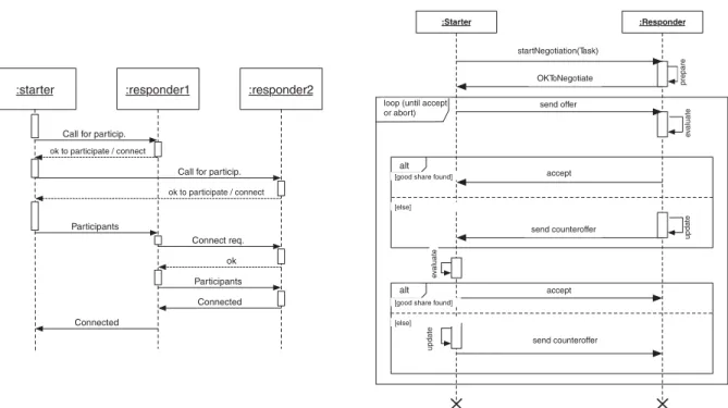
Figure 2. Connection protocol (left) and negotiation loop (right). The negotiation loop can be interrupted at any moment due to
an abort message of one part or a timeout when waiting for an offer (not shown in the sequence diagram for clarity).
We assume that the robots are willing to perform as much as they can of the given task (hence maximizing their reward), the only limitations being their available resources (endurance, computation power, battery consumption, etc.). Thus, in a negotiation, each agent will try to maximize its reward by (i) trying to get a subtask as big as possible and (ii) minimizing overlapping with other agents’ tasks.
The negotiation protocol is an extension of the
alternate-offersprotocol proposed by Rubinstein (1983). The advantage of such a protocol with respect to the contract net protocol is that in the contract net the auctioneer agent has to split the task into subtasks before placing the sub-tasks in the market, whereas in Rubinstein’s protocol the splitting is done during the negotiation. Additionally, each agent needs just to know whether the others agree with the share proposed for itself and nothing else.
In the alternate-offers protocol, each agent starts proposing the biggest possible share for itself and reduces it until the counterpart finds it acceptable. In this way a good near-optimal solution, although not optimum in general, can be achieved. The responder can agree with a subdivi-sion, or disagree with it, and in this case it has to propose a counteroffer. The protocol assumes a negotiation cost called
discount factor, by which it decreases its offers at each round, starting by claiming the whole good. Such a protocol has in-teresting theoretical properties: it guarantees a termination and can forecast the final agreement, which will be a per-fect equilibrium in the sense of game theory. An extension of the protocol has been necessary because it is not
imme-diately applicable to the multidimensional case. A detailed description of the process is outside the scope of this paper. We refer the reader to Rossi et al. (2009) for a more complete explanation.
Figure 2 (left) shows the connection protocol. Agents
are invited by thestarteragent in turn, and the list of agents
willing to participate is sent, in turn, to all participating agents in order to establish direct connections. In case of a lost connection during the connection stage and during negotiation, timeouts are used to interrupt the process. In case an interruption occurs, the protocol is restarted from scratch. Figure 2 (right) shows the communication protocol.
Only two agents are depicted for clarity. Thestarteragent
starts the negotiation, sending a request to the teammates
(only one is depicted). In case theresponderaccepts to
par-ticipate, a bargain loop is entered where the two parties al-ternately receive an offer, evaluate it, and decide whether to accept it, and in this case formulate a counteroffer. Note the search step performed at each new offer received and generated. The loop can be interrupted in any moment if one of the parties decides to unilaterally abort the negoti-ation in case a timeout occurs while waiting for a message or in case the mission is interrupted by the command and control station. When an agreement has been reached, the result is a subdivision of the original task and at the same time an assignment of the subtasks.
agents are satisfied the negotiation ends; otherwise another round is started. To avoid biasing the process in favor of the first agents, a new starter is chosen at each new round, in rotation. In this case, there is no theoretical result that guar-antees convergence of the negotiation. However, numeri-cal simulations with up to seven agents have demonstrated that an agreement is always found. Current work on this topic is devoted to a characterization of the convergence time as a function of the number of agents.
2.4. Communication and Computational Cost Issues
A final remark must be made regarding the communication topology implied by the algorithm. In this work, we have assumed that all-to-all communications are available in or-der for the negotiation to take place. All-to-all communica-tions are not strictly required, because in the negotiation rounds it is sufficient to establish a communication ring. Communications shall be available only during the nego-tiation itself and are not needed during the execution of the tasks the robots have agreed upon.
Bandwidth restrictions are not significant, as the amount of information exchanged is not a critical issue for our protocol. As an example, a polygon of 12 points is de-scribed by 24 floating point numbers. Assuming 4 bytes per number, a total of 96 bytes (plus headers) are sent at each of-fer. Taking into account the number of agents (three to five) and the typical number of negotiation rounds needed (30– 50), a total amount on the order of kilobytes for the whole process can be estimated.
Computational costs are centered on the proposal eval-uation and counterproposal update steps. Such costs de-pend on the application at hand. In this case each evalu-ation consists of computing polygon intersections and area calculations. A whole negotiation takes the order of sec-onds. In any case, we underline that in a distributed ap-proach such as the one we propose, each agent performs such computation only for its share, whereas in approaches that need to compute a complete solution, this cost must be multiplied by the number of robots of the team or by the number of subtasks that form the complete task.
3. PATH PLANNING
3.1. Problem Statement and Assumptions
The multi-CPP problem is formalized by assuming that there is a top-level procedure that handles the area division and the robot assignments. A cost-efficient multirobot CPP should result in a coverage path for every robot, such that the union of all paths is equivalent to the overall workspace coverage and the total coverage time to completion is minimized.
Let us consider an areaA⊂ 2decomposed in a finite
set of regular cellsC= {c1, . . . , cn}such that
A≈
ci∈C
ci. (3)
LetSbe a finite set of subareas andLa finite set of line
segments that divideA. ThereforeA=S∪L, where
S=
si∈S
si and L=
li∈L
li. (4)
In an aerial robotic–based coverage mission, the fol-lowing constraints must be considered subject to the vehi-cle characteristics:
• Nt: Number of turns, i.e., number of times the vehicle
rotates around the z axis (yaw angle movements)
• Nr: Number of times the vehicle covers a previously
cov-ered cell (revisited cells)
• t: Coverage time to completion of a single subareas
• T =ti∈Tti: Coverage time to completion of the
areasS
Letti∗=min{ti} be the optimal time for covering areasi.
Then the optimal time to completion ofS, T∗ is achieved
when all subarea coverage takes the minimum time:
T∗⇔t∗∀s∈S. (5)
Let us consider a coverage pathPto be optimal if it implies
the minimum number of turnsNtand of revisited cellsNr.
As explained later in this section, an algorithm that guar-antees that no cell is visited twice has been adopted, i.e., that Nr=0. Thus, P∗⇔min{Nt}. Clearly, ti∗ is achieved
with the minimum number of turns. Consequently, ti∗⇔
P∗. Then
T∗⇔P∗∀s∈S, (6)
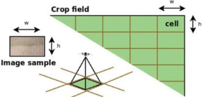
3.2. Area Sampling
The workspace is split through an approximate cellular de-composition. Following the taxonomy proposed by Choset (2001), the workspace is sampled like a regular grid. This grid-based representation with optimal dispersion is ob-tained by dividing the space into cubes and placing a point in the center of each cube. Therefore it can be defined as a kind of Sukharev grid.
Figure 3. Area sampling schematic. The required resolution and the FOV of the cameras determine cell size.
drawback that in general border cells may be partially occu-pied cells that must be visited, an exact cell decomposition such as the trapezoidal one is inefficient for aerial sampling because we are interested in acquiring an equally sized set of images.
3.2.1. Border Representation
Because the area partitioning algorithm works in a contin-uous space, borders (line segments) that define the subar-eas in the grid-based environment must be recomputed. In the grid environment, we represent lines using the Bre-senham’s line algorithm (BLA) (Bresenham, 1965), which belongs to the family of line drawing algorithms used in computer graphics. The procedure to approximate line seg-ments in discrete graphical data structures such as
rectan-gular grids of pixels is denoted asrasterization, whose goal
is to find the best approximation of a line segment given the inherent limitations of a raster environment, considering a set of constraints to be optimized (e.g., pixel proximity with the ideal line, continuity, and uniformity) (see Figure 4).
3.2.2. Subarea Identification
The procedure to individuate the subareas in the grid-based environment is a recursive flood-fill algorithm. The algo-rithm picks an empty cell (i.e., a cell not marked as occu-pied) and floods in four direction while there are empty cells, and each cell flooded is marked as occupied. When
Figure 4. Illustration of the solution based on rasterization.
the flood cannot go further, the algorithm is restarted. This procedure is repeated until all nodes of the grid are marked as occupied.
3.3. Coverage Path Planning
The CPP algorithm is performed for each subarea. We have developed an algorithm based on a wavefront plan-ner (LaValle, 2006) that works by propagating a wave front from the goal cell through all free grid cells bypassing all obstacles. A distance transform is applied over the grid by employing a breadth-first search (BFS) on the graph in-duced by the neighborhood adjacency of cells. Hence, the coverage path can be easily found from any starting point within the environment to the goal cell by choosing the nearest neighbor cell in gradient ascendant order, opposite to the conventional method.
The variables of interest in CPP areNtandNr(see
Sec-tion 3.1): a good path has a minimum number of turns and avoids visiting previously covered cells. Aerial robots have a certain endurance at a constant velocity, which is consid-ered a constraint (not a cost). Therefore, given an area, the cost to minimize is the coverage time, which fully depends on the number of turns and the revisited cells.
Because the number of cells in the grid-based workspace is known in advance, a simple way to ensure coverage completeness without revisited nodes is to use the deep-limited search (DLS), limiting the search depth to the maximum number of vertexes. During the gradient tracking, the algorithm can find more than one neighbor to choose from, with the same potential weight. A backtrack-ing algorithm builds a tree with all coverage path candi-dates and retrieves the one with the minimum number of turns.
4. AERIAL VEHICLE CONTROL
The last issue to be faced after the area has been partitioned and assigned and paths have been computed is the control of the vehicles.
Although nonlinear controllers have been used for some time for controlling quadrotors, poor analysis has been conducted on specifically improving attitude control while the aircraft is maneuvering at moderate speeds and performing aggressive changes in orientation. To improve on this, we have adopted the Frenet–Serret (FS) formula-tion as a set point funcformula-tion of the aircraft angular veloc-ity and acceleration. A complete and detailed description of the six-dimensional algebra operators, notation, and ba-sic concepts of rigid body dynamics applied to quadrotors modeling is outside the scope of this paper. The reader is
re-ferred to Section 3.2 of Colorado (2010)2and previous work
2Available for download at http://oa.upm.es/3493/2/TESIS
in Colorado et al. (2010) for a better understanding about
backstepping+FST derivation.
In summary, the backstepping+FST method focuses
on controlling the torque components ofτcm: rollτφ, pitch
τθ, and yaw τψ. This section briefly shows roll-control
derivation forτφ. The first step is to define the roll
track-ing errore1, and its dynamics (derivative with respect to
time):
e1=φd−φ, ˙
e1=φ˙d−ωx. (7)
A Lyapunov function3positive definite,V(e1)=e12/2,
is used for stabilizing the tracking errore1. The virtual
con-trol law for stabilizing the angular speed tracking error is then defined as
ωxd=c1e1+φ˙d+λ1
e1, (8)
withe2=ωxd−ωx. Includinge2in Eq. (8) and
differentiat-ing with respect to time (note thatωx=φ˙),
˙
e2=c1e˙1+φ¨d+λ1e1+φ.¨ (9)
Replacing ˙e1= −c1e1−λ1e1+e2 in Eq. (9) and with
Jx−cm,T the scalar component of thex-axis moment of
in-ertia of the vehicle,
˙
e2=c1
−c1e1−λ1
e1+e2
+φ¨d+λ1e1+Jx−-cm,1 Tuφ. (10) Note in Eq. (10) thatuφ=τφ. Solvinguφusing ˙e2= −e1− λ2e2, the control law is
uφ =Jx−cm,T e1
c21−λ1−1+e2(−c1−λ2)
+c1λ1
e1−φ¨d
. (11)
Likewise, for pitch and yaw stabilization,
uθ =Jy−cm,T
e3c22−λ3−1
+e4(−c2−λ4)+c2λ3
e3−θ¨d,
uψ =Jz−cm,T
e5c23−λ5−1
+e6(−c3−λ6)+c3λ5
e5−ψ¨d. (12)
Finally the terms ¨φd, ¨θd, and ¨ψd in Eqs. (11) and
(12), respectively, are replaced by the desired angular ac-celeration functions obtained using the FS formulation in Eqs. (13). The termω{{Ri}}is a 3x3resultant rotation matrix
that describes the vehicle’s trajectory orientation in terms of
3Lyapunov stability analysis of the backstepping+FST controller is
detailed in the cited work (Colorado, 2010, Section 4.3.5).
the FS frame transformation (see Colorado et al., 2010, for more details):
¨
φd =atan2ω{{iR}}23, ω{{Ri}33} ,
¨
θd =atan2
ω{{Ri}}13,ω{{iR}}232+ω{{Ri}}332
,
¨
ψd =atan2ω{R} {i}12, ω{
R} {i}11
.
(13)
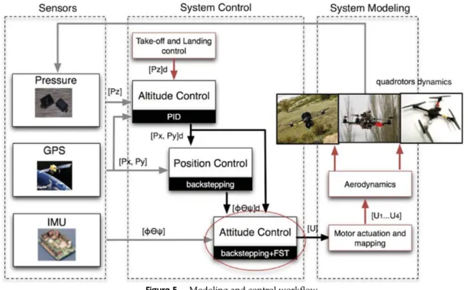
Figure 5 shows the modeling and control workflow.4The
system-control module is composed of a cascade-mode configuration of altitude, position, and attitude controllers coded onboard the vehicles. Appendix A shows a
compar-ison between backstepping+FST and a PID control.
The next section details experimental results con-ducted on both Hummingbirds and AR100 quadrotors. The analyzed data will show that our assumption of improving tracking speed is achieved by the introduction of the angu-lar acceleration function (based on FST) within the original backstepping control law. Those functions consider the ef-fects of the vehicle linear speed and acceleration, thus en-suring accurate and fast response to abrupt angular rate change, making attitude and position control more reliable when the quadrotor is maneuvering at high speeds (includ-ing strong wind disturbances).
5. EXPERIMENTAL RESULTS
In this section, the results of missions performed in a vine-yard farming site using the aforementioned system are pre-sented. The goal of the experiments is twofold:
1. To provide a useful field report in terms of using
this system as a practical approach for aerial sampling in precision agriculture involving a complex scenario (vineyard). Because vineyards are normally located in hilly regions, their shape can be quite irregular. In this case, area partitioning might not be trivial, and a sophis-ticated area partitioning algorithm like the one we are adopting provides a useful tool.
2. To demonstrate the simplicity and robustness of the
sys-tem architecture in terms of flight control and accuracy of crop field sampling.
First, we illustrate three different examples of the re-sults of the task partitioning and path planning steps on vineyards, in order to provide numerical results and illus-trate their outcome on different instances. The fields are
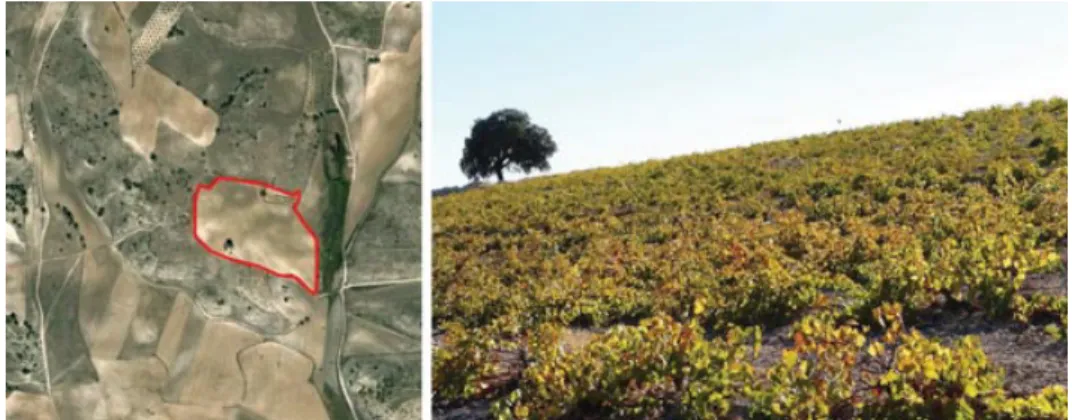
located in Belmonte de Tajo, southeast of Madrid, Spain.5
Figure 6 shows the three vineyards and the results of the
4Aerodynamics, dynamics modeling, and backstepping+FST
con-trol derivation can be found in Colorado et al. (2010) and Colorado (2010) with more detail.
5The authors gratefully acknowledge the courtesy of Bodegas
Figure 5. Modeling and control workflow.
area partitioning (left) and the corresponding paths gener-ated (right). Table II summarizes the results in terms of ne-gotiation round taken, elapsed time for the path planning step, number of turns, and quality of service obtained (see below for a definition).
The vineyard-field chosen for the field tests was Field 1. Its location is depicted in Figure 7, with the area to be covered delimited by a thick line. This crop field
sce-nario has an approximate size of 327×195 m.
To evaluate the experimental results according to the goals previously mentioned, we introduce a set of metric variables. These metrics are conceived in order to analyze
the performance of the vehiclesduringandafterthe mission.
Tables III and IV summarize these metrics:TMis the total
mission time, including deployment and setup time;TLis
the setup time;TCis the total flight time;TEis the time the
vehicles are actually flying between waypoints;T¯E is the
time the UAVs spent hovering over a waypoint; andPis
the length of the coverage path.
Table II. Summary of the results for task partitioning and path planning.
Negotiation Total path Total no. Quality of Field rounds planning time (s) of turns service (%)
1 36 0.19 37 72
2 43 0.22 42 81
3 49 0.31 36 80
Table III. Metricsduringmission flight.
Variable Description
PE Position error tracking
HE Altitude error tracking
VW Wind disturbance
Table IV. Metricsaftermission flight.
Variable Description
TM Mission time of completion
TL Grounded time
TC Coverage time of completion
TE Effective time of coverage
T¯E Noneffective time of coverage
P Coverage path
Finally, because subarea borders will not be sampled,
an end user–oriented metric called thequality of service
in-dex is measured, which indicates the percentage of the
field actually surveyed. An upper bound (UB) of unvisited
cells can be estimated for the security strips as follows. For
simplicity, let the area be discretized in an N×M grid,
Figure 7. The vineyard crop field object of the field tests. Its location is 40◦1124.68N, 3◦2856.09W.
Figure 8. The aerial vehicles flying over the agricultural scenarios.
the number of robotsR. The maximum length of a line is
equal to the diagonal. In a discrete world, the length in cells
of the diagonal is equal toM; hence,
UB=
R·M N·M =
R
N. (14)
We refer to the valueUB/(N·M)(%) as aquality of service
index. In our experiments,N=M=10;R=3, and a
maxi-mumof 30% of the cells will be security zone and therefore
will not be visited (actual values range from 20% to 30%; see Table II). Note that in crop field sampling, 100% sampling is not needed. Conventional sampling methods currently used are based on far lower sampling rates.
5.1. Platform Overview
Experiments were carried out using a team composed of three quadrotors: (i) two Hummingbird quadrotor
platforms6 and (ii) the AR100 platform.7 Prior to the
description of the experimental setup, this section briefly
6Ascending Technologies GmbH, http://www.asctec.de/. 7AirRobot GmbH & Co. http://www.airrobot.de/.
introduces some description of the platforms employed. Both platforms are shown in Figure 8.
The mainframe of the Hummingbird is composed of an AutoPilot board that includes (i) a LPC2146 ARM high-level (HL) processor, (ii) a triple-axial compass for mea-suring the vehicle’s heading, (iii) as inertial measurement unit (IMU) and pressure sensor from attitude and alti-tude measurements, (iv) a GPS unit for geolocalization, and (v) low-level X-BLCD brushless motor controllers. Using the Software Development Kit (SDK) provided by Asctech,
our backstepping+FST runs onboard the HL processor
us-ing a sample rate of 30 samples per second. The GPS po-sition loop is set at 1 Hz, whereas the IMU loop is set at 100 Hz (the maximum transfer rate of the IMU data can be set to 1 kHz using the serial interface). All data generated by the IMU are sent to the ground PC station via wireless data link (XBee 2.4-GHz module) for data analyses and user visualization purposes.
Table V. Aerial fleet parameters.
AR100 Hummingbird
Diameter (m) 1.0 0.63
Weight (kg) 1.32 0.6
Payload (kg) 0.25 0.2
Autonomy (min) 20 25
Wind load (m/s) 8 8
Max. velocity (km/h) 50 50
platform stabilization, manual control, and waypoint nav-igation, as well the dispatch of the commands from a soft-ware mission planner set in the ground station, which en-ables the operation of the robot at a higher level.
A summary of the technical data of the two platforms appears in Table V.
Theground stationis composed of the communication devices and a graphical user interface (GUI) for real-time information of the mission. For the AR-100 quadrotor, a graphical interface was developed to fulfill the needs of a friendly-user experience. On the other hand, the Hum-mingbird already provides a GUI that enables some ba-sic functionalities for mission supervision. Figure 9 shows the base station for the experimental setup and the GUI of both quadrotor platforms (left for the AR-100, right for both Hummigbirds).
In terms of communication architecture (see Figure 10), the base station computer receives and send data to AR100 through a RS-232 downlink and uplink that operates be-tween 2.3 and 2.5 GHz. The quadrotor can also be teleoper-ated through a radio control (RC) system that relies on nine available channels and operates at 35 MHz. Additionally, a video transmission downlink at 688 MHz is also set to re-ceive video images acquired by the digital camera. For the
Figure 10. Air–ground communications architecture.
Hummingbird, the vehicle sends and receives data through the base station through a X-Bee Datalink that operates at 2.4 GHz, as previously mentioned. In terms of user super-vision it is important to highlight that the mission can be manually aborted using the GUI. For this reason, two pro-cedures can be followed: (i) the quadrotor has to remain in hovering maneuver waiting for manual flight or (ii) the quadrotor will return to the home point (beginning of the mission) autonomously.
5.2. Experimental Setup
Recalling the workflow of Figure 1, the steps followed in order to performed a survey mission are as follows:
1. The operator defines the target mission field by selecting
the area’s vertices on a georeferenced image.
2. The vertices are passed to the negotiation algorithm,
which produces the area subdivision and assignment (at this stage, the characteristics of the robots employed such as endurance and the cameras’ FOV are hard coded in the workflow).
3. The subareas are discretized and then the areas’ bounds
are computed, taking into account the required resolu-tion and camera parameters.
4. Cells containing obstacles (e.g., water well, irrigation
systems) and subareas bounding cells are marked as no-fly zone.
5. Coverage paths for each subarea are calculated.
6. Flight plans (list of waypoints) are sent to the robots.
7. Mission is simulated (optional step using a
Matlab-based simulator depicted in Figure 11).
8. Mission starts.
Given the limited sensing and processing capabilities of the robots employed, direct perception for avoiding col-lisions during flight is not feasible. On the other hand, com-munication of the positions is not feasible because vehicles do not have direct communication during the mission, and indirect communication through a base station is not rec-ommended due to a high risk of radio interference.
Thus, with simplicity and effectiveness in mind, colli-sion avoidance is achieved through two basic principles:
• Different vehicles fly at different altitudes.
• Subarea bounds define a security zone: vehicles are not
allowed to enter it.
5.3. The Vineyard Field Experiments
5.3.1. Experimental Setup and Preflight Phases
Figure 11. Steps performed for a real mission.
This complex environment was inscribed in a rectan-gle [see Figure 12(a)]. Therefore, the workspace for this
ex-periment was defined as a 63,765-m2rectangular area (see
Figure 7), where general parameters are set up as follows:
• Field size: 330×200 m
• Grid size: 10×10 cells
• Cell size: 32.7×20 m
According to the workflow, the first step in the pro-cess is to divide the workspace into as many adjacent ar-eas as quadrotors available. Figure 6 (top, left) shows the three subareas resulting from this step. Next, flight plans are generated [Figure 6 (top, right)]. Table VI summarizes the results of this step. When a mission has been simulated and the parameters for the CPP have been validated [Fig-ure 12(b)], configuration data are sent to the corresponding drones. The strings containing the waypoints for each mis-sion are loaded into the scheduler of the drones, waiting for the mission start signal.
Table VI. Details of the results obtained from multi-CPP on the vineyard parcel chosen for the field tests.
Area 1 Area 2 Area 3
Turns 9 8 20
Computation time (s) 0.15 0.02 0.02
Note that the actual target workspace consisted of 65
of the 10×10 cells of the area, 12 of which would not be
sampled because they formed the subarea boundaries [cf.
Figure 6 (top)]. Thus, thequality of servicein this experiment
has been 72% (18% of the area was not sampled).
5.3.2. Flight Results
Figure 12. Detailed experimental workflow results of three quadrotors performing vineyard field sampling and coverage. Labels AV-1 and AV-2 correspond to the Hummingbird UAVs, AV-3 to the AR100 UAV.
Figure 12(c) shows the results of one test mission flight. In the following, we analyze the outcome of this test.
The main requirement that aerial vehicles must accom-plish for a reliable imaging survey is to have an accurate three-dimensional (3D) positioning and be able to perform smooth trajectories. This is important because the vehicles have to acquire a set of georeferenced images that will be postprocessed by an image mosaicking procedure in order to build a map from the crop field surface. Owing to its relevance on this mission, the first parameter analyzed is altitude. Altitude accuracy plays an important role in imaging surveys, because the image samples must be taken from the ground at a determinate constant altitude. The relationship between the camera FOV and the aerial vehicle
height above the ground is given byτd/τh=Id/ l, where
τd, τh, Id, and l stand, respectively, for cell dimension,
aerial vehicle height, image dimension, and focal length of the camera.
In Figure 13 (right) the altitude evolution for each quadrotor during the flight is shown. On the left, the corre-sponding Cartesian paths are plotted. As expected, the
flat-ter surface provides betflat-ter results (see plot for quadrotor 1, Figure 13, right, top). Altitude control also has a direct ef-fect on battery evolution, reducing peaks and maintaining a more stable discharging process. The mean altitude had a maximum error of 3.35%, as shown in Table VII, which is acceptable for an outdoor mission in which the platforms are constantly subject to prevailing winds.
Errors in altitude location are not directly related
to accuracy in navigation over the XY Cartesian plane.
Figure 14 shows the results obtained in position tracking. Compared to the paths shown in Figure 14 (bottom), where real paths are superimposed on the theoretical paths on workspace assignment, maximum errors are related to sud-den variations in the quadrotor’s yaw axis (orientation). The best example comes from the tracking error on zone 1. In this flight, note an error increase of almost six times in four moments (tA=0.05 min,tB =0.65 min,tC =1.2 min,
tD=1.4 min) when the quadrotor faces acute angles. This
0 50 100 150 200 250 300 350 0 40 80 120 160 200 X [m] Y [m]
0 1.5 3
20 21 22 23 24 H[m]
0 1 2 3
10 10.5 11 11.5 12 b[v o lts]
0 2.5 5
26 28 30 32 34 H[m]
0 2.5 5
10 10.5 11 11.5 b[v o lts]
0 3 6 9
26 28 30 32 t [min] H[m]
0 2 4 6 8
9.5 10 10.5 11 11.5 t [min] b[v o lts] Altitude quadrotor−1 quadrotor−2 quadrotor−3 Battery Altitude Battery Altitude Battery
Figure 13. (Experimental) Cartesian path (left) and altitude tracking and power consumption during flight (right).
more yaw drifts, presents a position error greater than the area with fewer turns (zone 2) (see Table VII). Table VII also
permits a first comparison between our backstepping+FST
controller and the commercial PID-based controller of the
AR100 UAV. ThePEerror for UAVs 1 and 2, adopting our
controller, is smaller than the error for UAV 3. UAVs 1 and 3 have a similar error, but note that UAV 1 was flying at a higher speed. This comparison is done on different paths and different areas. Appendix A illustrates a more fair comparison between the two controllers under equal conditions.
As far as flight speed accuracy is concerned, prelim-inary tests have been done through simulations, with the purpose of helping the design and tuning process of the AV controllers. During the simulations the vehicles were
subject to wind speeds of 10 m/s in both thexaxis and the
y axis. The vehicle dynamics during the simulations
per-formed well. However, real performance was not as good as expected. The reason for this behavior is the winding streams the vehicles are exposed to. Such winds are typi-cal in hilly zones and can achieve peaks much greater than
10 m/s.8. For the purpose of our mission this drawback
can affect a system in two ways: when a vehicle is hover-ing over a waypoint, because the drone must maintain its
8On one occasion, a strong wind stream lifted one vehicle to>
100-m altitude. The vehicle eventually landed so100-me 500 100-m away fro100-m the base station.
Table VII. Summary of the metrics measured during the flights; flight took place on March 21, 2011, 15:20 hours, Spanish time.
href h hE Vref V Vwa PEb UAV no. (m) (m) (%) (m/s) (m/s) (m/s) (%)
1 20 20.67 3.35 5 3.22 13 2.3
2 30 28.95 3.50 5 2.97 13 1.5
3 30 28.69 4.30 5 2.41 13 2.5
aWind speed measured at base station.
bError accurately measured using Vincenty (1975) formula.
position to provide a clean and accurate image, and when flying between waypoints, because the vehicle shall per-form a smooth trajectory in order to optimize flight time and power consumption.
Figure 15 shows a comparison between the simulated and measured velocity profiles generated by the controllers during the test mission.
Another important detail in a coverage mission is the overall time of completion. Overall completion time can be decomposed into coverage time and setup time. Moreover, coverage time can be decomposed into effective and nonef-fective time.
Figure 14. Position tracking during flights. LabelstA, tB, tC, andtDrefer to peaks of the tracking error.
mentioned factor, the human efforts for mission setup. Al-though the AVs are full autonomous platforms, each one must have an experienced pilot and/or a ground base op-erator who supervises the mission. In this sense, we are adopting a configuration similar to the one proposed in Murphy and Burke (2008), in which a pilot is in charge of supervising (and, if necessary, teleoperating) the UAVs
and a mission specialist is in charge of supervising the
mission. The typical and safer modality is to have two persons in charge for each drone. The pilot is responsible for supervising the mission from the ground and switches from the automatic to manual mode in case there is some system failure or emergency. The base-station operator is in charge of supervising the mission at the highest level (i.e., monitoring all the navigation data in real time). Al-though there is no specific security legislation applied to mini aerial vehicles, this measure is mandatory for safe experimentation.
The mission presented here was carried out by three pilots and two base-station operators. Table VIII shows the time dedicated before and after the mission with the AVs. This includes preliminary flights and communication tests (e.g., ensuring that the corresponding ground stations are correctly receiving and sending data). It is interesting to ob-serve that the setup time increases with the area of coverage (i.e., geographic area).
As mentioned before, the coverage time is composed of an effective and a noneffective time. The effective time is the absolute time the aerial vehicle is moving between way-points until the final coverage trajectory is performed. The noneffective time is the overall time hovering over the way-points. The results obtained also show that both effective and noneffective times increase with the number of way-points per subarea.
The results of the field tests performed can be summa-rized as follows:
• The accuracy of the navigation in theX–Y plane is
af-fected by the kinds of turns.
• The coverage time increases with the number of turns
and the number of waypoints (however, note that the number of turns is not necessarily related to the number of waypoints).
• Depending on the region where the mission will take
place, peak wind stream velocities must be quanti-fied and taken into account for good speed tracking. Simulation and tuning of the controllers shall take these into account.
• Around 50% of the overall mission time was devoted to
system assessment and setup.
• Even if highly autonomous UAVs can be currently
ob-tained off the shelf, efforts are still needed as far as us-ability and safety for their effective use for commercial applications, especially when multiple UAVs are to be employed.
Table VIII. Summary of the metrics measuredafterthe flight.
UAV TE T¯E TC TL TM Pa Batteryb
no. (s) (s) (s) (s) (s) (m) (%)
1 141 42 183 282.76 465.76 373.74 7.64 2 151 45 196.43 81.85 278.28 339.75 8.399 3 213 75 288.02 313.25 601.27 650.52 12.39
aInformation obtained from a georeferenced image with a
preci-sion of±3 m.
bRelative battery consumption.
6. DISCUSSION AND CONCLUSIONS
In this paper, a practical solution for performing aerial imaging applied to precision agriculture by using a fleet of UAVs has been presented. This paper provides a unified view of the work we have been carrying out in different fields: multirobot task planning, path planning, and UAV control.
A simple and efficient strategy for the coverage of a crop field using aerial robots for data collection has been presented. The approach proposed includes two steps: in the first step a given area is subdivided by the team robots and each robot is assigned a subarea. In this phase the robots are aware of each other and carry out this task cooperatively. The second phase handles the workspace sampling and the coverage planning. In this phase the robots are unaware of each other and parallel path plan-ners compute the coverage path for each robot. Finally, a robust flight controller drives the AVs through the mission.
The area partitioning and assignment distributed algo-rithm is capable of taking into account the characteristics of different vehicles, a feature useful in the case of heteroge-neous fleets. The methodology employed for path planning guarantees finding an optimal solution if one exists, provid-ing coverage paths with minimal turns to the aerial robots, ensuring that cells are not visited twice, and including fixed
and known obstacle9avoidance.
The planning step introduces security boundaries be-tween subareas assigned to the vehicles. These should be carefully optimized in order to ensure suitable quality of service and at the same time guarantee the security and safety of the platforms. A way to get rid of the safety strips that are mainly responsible for reducing the area covered would be to take into account the cell dimensions in re-lation to the AVs’ position accuracy and the probability of having two or more than two AVs flying at the same time in adjacent cells, analyzing the flight plans prior to the
9For instance, irrigation systems or other obstacles such as
beginning of the mission. In other words, a mission val-idation step, using the optional simulation tool, could at the same time eliminate the need for no-fly security strips and ensure collision-free missions. Alternatively, achieving 100% coverage will involve the integration of temporal con-siderations in the planner in order to always respect a safety area around the UAVs, for instance using a validating plan-merging operation (Gravot & Alami, 2001).
As shown by the field tests, reducing the number of turns is extremely important because turns affect both mis-sion time and, more important, the precimis-sion of the 3D po-sitioning. We can also conclude that, contrary to what was expected, position error is less affected by the speed of the vehicle.
As far as control is concerned, it was possible to assess
the performances of the backstepping+FST technique
adopted by the Hummingbird robots (in substitution for their original one) in comparison with the AR100
controller. The backstepping+FST technique has shown
better robustness against large disturbances as model un-certainties were canceled thanks to integral action and the incorporation of FS theory. Precision during tracking was also improved. This feature clearly plays an important role
inopen fields, where the vehicles are exposed to rapidly
changing conditions.
The field tests have also shown that local conditions (in this case, the different slopes) must be carefully taken into account because they can generate wind streams far more rapid than the maximum wind velocities used in simula-tions and measured at the base station. This is especially true in wide areas. This aspect did not appear in other field tests (e.g., cornfields, tests not reported here) due to the simpler orography of the terrain.
Although not applied yet, orography information can be incorporated in the planning stage, by adding preference terms to the cost model of the vehicles during the negotia-tions. Information regarding particular terrain-dependent wind conditions in given regions would be treated in the same way as in no-fly zones: vehicles would be denied to fly over regions where expected winds would overcome their limitations.
In general the operation protocol workflow has worked well, providing a smooth tool from area definition to mission execution. The decoupled area partitioning and path planning steps allow for different partitioning to be generated and examined by the operator prior to mission execution. Also, after path planning has been performed, the mission simulator allows simulating and validating the mission beforehand.
However, we would like to point out that even with a well-structured operations protocol and with highly au-tonomous robots (capable of taking off, performing the mission, and landing back to base autonomously), the re-sources needed for deploying the robot team and setting up the whole system play an important role. As far as human factors, with three UAVs at least four persons are needed
for a safe mission: one backup pilot for each vehicle plus one mission supervisor at the base station. As far as mis-sion time is concerned, deployment time was about 50% of total time for a single mission.
This is only partially due to the fact that the system is not currently thought out for the end user, and its operation has to be done by technical staff. Much work will be needed in order to provide a simple and safe system to be operated directly by farmers, especially in terms of a unified, friendly GUI that provides task definition and mission execution monitoring by untrained persons. For this reason, our view is that a multi-UAV system as a farming tool such as the one presented here would be better exploited commercially by a company providing services (system plus technical staff) to different farmers in the same area.
Finally, it is important to remark upon the unified vi-sion provided by this work. In the literature a number of papers can be found that regard either task planning path planning or UAV control, but few works provide a com-prehensive analysis of a whole system, from the theoretical study of the individual technical issues to a complete field experimentation.
7. APPENDIX A: BACKSTEPPING+FST CONTROL
To assess the assumption of improving flight control
us-ing the backsteppus-ing+FST, this appendix shows
simula-tion tests related to the accuracy of the aforemensimula-tioned controller against a PID control in terms of disturbance rejection (strong wind). Many commercial autopilots use PID methodology that is capable of controlling the sys-tem during certain conditions, such as hovering or flight without the presence of strong perturbations. However, as experimentally demonstrated in Bouaballah (2007) and Olfati-Saber (2001) and also in previous work (Colorado, 2010), PID controllers are capable but not efficient in stabilizing the aircraft (in terms of attitude control) when nonlinearities produced by Coriolis accelerations play a significant role. This is produced when large disturbances cause changes in velocity that result from rotation. PID con-trollers have proven to be well adapted to the quadrotor
when flying near hover, but the backstepping+FST is
ca-pable of faster attitude stabilization mainly because of the introduction of the terms ¨φd, ¨θd, and ¨ψd within control laws (11) and (12) respectively, which consider the effects of abrupt angular changes while flying a moderate speeds (FS foundation).
Figure A.1 shows the cornfield scenario. Flying at rela-tively high altitude (considering the sizes of the AVs), wind strength and gusts play a fundamental role. Hence, one of the main goals, as far as control is concerned, is to analyze how the controller is capable of stabilizing the system when strong wind disturbances are addressed.
Figure A.1. (Simulation) control performance in terms of position tracking under strong wing perturbations. Backstepping+FST against PID.
Table A.1. Summary of the metrics measured during simulation.
href h hE Vref V Vwa PEb
No. (m) (m) (%) (m/s) (m/s) (m/s) (%)
PID 1 20 20.04 0.2 2 2.3 10 2.5
2 20 20.12 0.6 5 4.8 10 8
3 20 20.2 1 10 9.8 10 23
BS+FST 1 20 20.04 0.2 2 2.05 10 1.2
2 20 20.08 0.4 5 5.2 10 3.8
3 20 20.17 0.85 10 10.3 10 6.7
aWind speed introduced as a force disturbance. bAverage tracking error.
the backstepping+FST approach by measuring the
posi-tion tracking of the trajectory within the circle. In addiposi-tion, Figure A.1 also details the results of the Hummingbird fly-ing at 20-m altitude and average linear speed of 5 m/s.
On average, the PID obtains maximum position tracking
errors up to 8%, backstepping+FST about 3.8% under the