Triomensional plasticity using BIEM

Triomensional plasticity using B I E M

F . G. Benitez and E. Alarcón

Escuela Técnica Superior de Ingenieros Industriales, Madrid, Spain

C. A. Brebbia and J. Telles

Department of Civil Engineering, University of Southampton, Southampton SO05NH, UK

This paper presents the application of BIE techniques to elastoplastic three-dimensional problems. Along with the general procedures the needed ¡ntegrations are described ¡n detail and so is the flow chart of the written program.

Introduction

It is well known that the Boundary Integral Equation Method (BIEM) can be based on a reciprocal relationship between two elastic states. In our case, we shall take an auxiliary one defined by the fields (o,*, Ef¡, uf) and the elastic part of the increment of deformation components in an elastoplastic system {b¡¡, f;,«,-).

Thatis:

or:

Jaíéf

dK=Jeíá

dF

D D

lF,*ü¡dV + ÍT,*ú¡áS

D dD

= \F¡uf áV+ \t,ufáS+ \afkéfkáS

(O

D dD

Taking the (*) system as that corresponding to the Kelvin solution, that is:

Fi* = 6(x-x)el

T? = T,¡e, uf = u¡te¡

aik ~ ^jikej

we obtain:

ú¡(x)+ I TjiúiáS

dD

=

dV + I tilín áS + J 2

éf

dV (2)

xGD

dD

which is a representation formula for the incremental displacement at an interior pointx.

By the usual limiting procedure, equation (2) can be transformed in:

c//"/(*) + J Tj¡ú¡ dS &,*w -ik

= I Uji'tidS + i iijiFidV + j 2//fc xGdD ₍₃₎

dD

The first domain integral on the right hand side can be expressed as a boundary one for several useful cases (self-weight, centrifugal forces, thermoelasticity, etc.) in the form:

I itjiFi dV=\ 0ÍÍ///2,- dS + í Sl¡ - dS - í 4> — ' dS

(4)

dD _ao 3D

-k0 í Wj¡n¡dS

3D with:

F=V<p k0 = V>4>

Í2; 1 — 2P

; \6TÍG{\-V) •'

3í2y I - 2v

— = T ¡knk

3ii 167rG(l-i;) ,;*

Inside the body under study: 2Gv

(5)

\-2v where:

tt..= ti*e + IPP

Assuming:

we obtain the following material law: 2Gv

Oij = p - ^ S' V < » .+ G("U + "Áf) ~ 2Geü ( 6 )

After some algebra, the introduction of (2) inside (6) pro-duces:

a„ = f D

t

áS - ís

ú

áS + JD

F

dV

D

i-ñD

+ | s/ / H

P,áV-W D

7-Sv

2G<£P 15(1-1») "

In tliis expression, it has been necessary to use the principal valué of the plástic singular integral developed by Bui and Mikhlin/thatis:

9

dxh

Js^ek

, ?>omlv . n 8 —lOf . „ dxh 'lv'

D D

15(1-1/) mfc

The discretization of the above written equations can easily be obtained when we assume a constant valué of the functions on boundary elements as well as inside cells in which the whole domain is divided.

The final results are:

N.EIe.

L = l

N.EIe. N.EIe. N.Cel. = £H//2}(¿)+ I ho+ Z Eflk€fk(AI)

L = \ L = \ M=l

K,MGD,LedD

N.EIe. N.EIe. a/y(m)= £ 'nkijtk(Q- £ 'fujútiL)

N.Cel. N.EIe. + £ E/lkiék'l(Af)+ £ /¿D

J l í = l AT=1

7-Sv

1 5 ( 1 - P )

2G¿jJ(M) K,LGdD,AieD

1 N.EIe.

-«/(*;) + X £/,«,(£.)

2 L=\

N.EIe. N.Cel. = £ « , , / , ( £ ) + 2 /8 D + I ^ifcCf^AÍ) (9)

¿ = 1 A / = l

Figure 1 Integration f r o m points contained ¡n cells where integral

¡s belng carried. a, boundary equation (3) A B C D = A B O D U ABOC U A C O D . b, ¡nternal stress, equation (7) A B C D = OABC U OBCD U OACD U O A D B

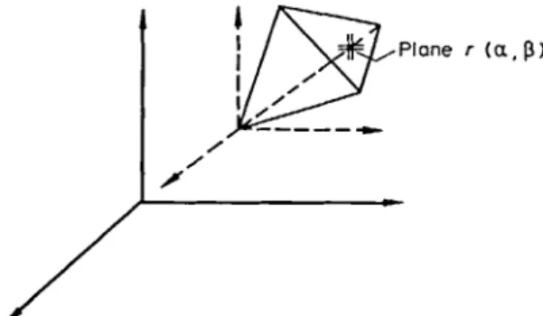
Plañe r ( a , (5)

( 7 ) Figure 2 Tetrahaedron, D¡. / , = fo¡^kij d v

where there is an obvious correspondence among the capitals ÍT, 51, «2, D, Jf and the integráis with kernels T, U, 2, D, S and where N.EIe. and N.Cel. means 'number of elements' and 'number of cells', respectively and:

N.EIe.

L = \

N.EIe.

L = l

*• ' represent the discretization of the (4) expression.

Computation of the coefficients

None of the boundary integráis presents any computational difficulty and the procedures used in elastic Solutions can be utilized without difficulty. This is why we shall concén-trate on the analysis of the volume integráis corresponding to plástic deformation. To compute those coefficients the domain D is divided into tetrahaedrical cells in which the valué of CP is assumed to be constant.

There are several cases, among which we shall distinguish two groups: when the integration is carried from points contained in a cell or when it refers to a point far from the cell.

The first category can be reduced to a simpler problem of whether the point is on the cell boundary or inside it {Figure 1). Taking the point as a vértex the cell can be divided into three {Figure la) or four {Figure Ib) sub-domains in which the common feature is that the integral has to be carried from a vértex of a tetrahaedron.

The second category is generally computed by numerical methods, while the first is done by semianalytical methods. Let us discuss this later problem. The integration from boundary points is:

I^jz^dV

Di where:

2fcf/ ~~ 2 fkij

3C3 fki¡ = (5jfc,-r,/ + 8kjrj - 5 urt k) + rt ¡rtlry k

Ci =

\-2v

C,=

8JT(1 -v) \-2v so that, integrating in D¡ {Figure 2),

(11)

h = - c

SU?

a 0

= ~C1 f I [ /W /c o s | 3 dad/3 (12)

where r ( a , /3) represents the equation of the face opposite the vértex from which the integration is done.

Changing to a system of natural coordinates (Figure 3) contained in that face:

A = surface of 123

P(Xp;yp;Zp)

x

Figure 3

be utilized without difficulty. This is why we shall concén-trate on the analysis of the volume integráis correspondong to plástic deformation. To compute these coefficients the domain D is divided into tetrahaedrical cells in which the valué of C is assumed to be constant.

There are several cases, among which we shall distinguish two groups: when the integration is carried from points contained in a cell or when it refers to a point far from the cell.

The first category can be reduced to a simpler problem of whether the point is on the cell boundary or inside it we have:

dad/3 = 2/1

r2 eos /3

and so:

dSi d%2

h = -2ACx f f - /Wy d 5 , d {2

í ' = l

(13)

where W¡ are the appropriate weights for a numerical Hammer quadrature.

The other case is the integral needed for the equation (7) of internal points. In this case:

-i

I2=\ ZmdV

D where:

_C G

or:

gijki = 3(1 - 2v)(b¡¡rykr¡t + &k¡rtirj)

+ 3(5//r?/r>fc + Bjkrtlryi + b¡kr,¡r,¡ + Spr^r^)

- 15rf,rt /r,, + (1 - 2i>)(8¡k8,j + SJk6„)

- ( l - 4 « 0 5/ y8w (14)

¡Di = J -¿S ¿9 = j j | 3gr2 cos/3 da d/J dr

D/ a p t£

= C f [ lnrg cos/3 da d / 3 - C l n

- C l n £ j f^ cos/3 da d/3

a (3

Summing up the contributions of the four tetraedra confluenting in tliis vértex, the second integral will be defined inside a sphere of radius £.

As:

(15)

r,ir,f c o s^ ^a ^ = ^Ü ~ W

•a 0

we obtain:

f (g cos/3 da d/3 = 0

and the integral will be:

I2 = C f flnrg cos/3 do

r

fin/-e d/3

d|2

(16)

(17)

a (3

which is solved numerically in the same way as It.

In the previously called 'second category', that is, when the integration point is far from the cell, the computation is done numerically from the beginning. That is:

/,' = f 2W / dV~- C, j-AijGVd^ dfc d?3 (18)

D and:

4JT(1 - v)

I'i = j ^ijkIdV-cj~g6Vd^d^dh (19)

D D

Iterative procedure

The establishment of equations (9) for as many points as elements on the boundary leads to a system:

H.ú = G.¡ + Í + D<£p (20)

and for internal cells:

ó = G'i-II'ii+Í' + (D' + C')ep (21)

Ax=F+D£p

ó=Áx+F" +D*-£p

(22)

(23)

H' is the tangent to the curve equivalent stress versus equivalent strain.

or:

x=A-1F + A-íD€p

Ó^A'A^F + A'A^DVP+F' +D*€p

In compact form: x=M + k£p

ó = Ñ + B£p

As (26) represent incremental valúes, it is possible to write, for a step/:

0 0 0

o

?/ = I ó* + á/ = I A \ - + ¿ I eg + A7,-+Bef

0 0 0

Program characteristics

(24)

The numerical process, presented above, has been developed (25) in a FORTRAN V program and implemented in a UNIVAC

1108. The mean properties of this program are: (1) It uses a constant interpolation function for the displacements, stresses and plástic strain fields.

(26) (2) I *u s e s ^a t triangular elements in order to discretize the

boundary of the domain.

(3) It introduces tetraedral cells with flat faces to discretize the plástic part of the domain.

(4) It considers homogeneous and isotropic materials only. (5) It is possible to take volume loads into account. (6) It is possible to take concentrated loads such as those corresponding to prestressing cables into account. (7) Materials have been considered for which the incom-pressibility of plástic strains (metáis, clays) is accepted. (8) The strain-hardening model that has been used is the isotropic one.

/ - i

• \¡N+B £ e£ + e? (27) The main parts of the flow chart of the programe are described below:

or:

x¡ = XjA/ + *(<£" + A£p) o¡ = hN+B(£p + Afi")

(28)

where M and N are elastic boundary and domain solutions and X/ the corresponding load factor. The iterative proce-dure is clearly shown in the flow chart contained in the next paragraph, where :

oe is the equivalent or effective stress (Von Mises criterion).

ae = - \{ox - oy)1 + (ox - azf + (ay - azf

Input data Print data

+ 6{Txy + TX2Z + ry2z)]

a?13" is the máximum valué of ae in the whole domain:

F'-=E?+

AEP-e'ij ~ E'ij ~ ~E'kkh¡

Eet is the modified equivalent deformation:

l • •

et ei¡eij

A£„ =

?-±

AEp

.-^e'.-K

Computation of integral coefficients for elastic case Generation of equation system for elastic case

\

Boundary conditions I

Computation of elastic solution X = M

i

Computation oí A, I,D and K matrices

I

Computation oM'.A'and U matrices i

Vector displacements in internal cells for elastic solution

Print elastic results i

Computation of matrix D and B=D*+A'K

i

Read o0, WandM

l Iterative process Computation of plástic strains

in internal cells

Print results u,t, a i

End

Iterativa process _References

Initialization of plástic strains

pr = O and ¡ncrementols A P. =0

For eoch cell

6 ij = X; • n • B • EP

i

Computes Te and H'

1

d>

AE//=0

Computation of

^ ' e'ij • Eet . A f p . hEfj

Comparison between Jast valué of AE,y and previous one

0-

^MD

END YES

10

11

Bui, H. D. Solids Struct. 1978, 14, 935

Banerjee and Mustoe. 'The boundary element rnethod for two-dimensional problems of elastoplasticity'.

Banerjee et al. In *Two and three-dimensional problems of elastic-plasticity methods - 1', Banerjee, Butterfield, App. Sci. Publishers, 1979

Kumar and Mukherjee. 7/if. J. Mech. Sci. 19,713 Mendelson. 'Boundary-integral methods in elasticity and Kumar, . . and Mukherjee, . . Int. J. Mech. Sci. 0000, 19, 713

Mendelson, . . 'Boundary-integral methods in elasticity and plasticity'.NASA TND, 7418,1973

Mendelson, A. 'Applications of boundary integral equations to elastoplasticity problems', Boundary-integral equations rnethod: computational applications in applied mechanics, Cruse and Rizzo, ASME, 47-84,1975

Morjaria and Mukherjee. Int. J. Numer. Meth. Eng. 1980,15, 97

Mukherjee and Jumar. J. Appl. Mech. 1978, , 45 Swedlow and Cruse. Int. J. Solids Struct. 1971, 7,1673 1673

Telles, J. and Brebbia, C. A. Appl. Math. Modelling 1979, 3, 466

Telles, J. and Brebbia, C. A. New development in boundary . element methods' (ed. Brebbia, C. A.), CML Publications, Southampton, UK, 1980

Appendix

Tensors

Here we present the Kelvin solution and the associated tensors, which have been used in previous equations. If we define:

x: Point where the concentrated load is applied y: Field point

r: \x-y\

we willhave:

Conclusions

This paper presents the application of B.I.E.M. to tri-dimensional plasticity and its implementation on the computer. This theme is being developed at present for more complicated cases at the Polytechnical University in Madrid and the University of Southampton, by the present authors and other members of these groups.

A U )

Notations

9

x

E^Ef.+EZ

%

E?i

'/(*) Xk

°ij(x)

«// (*) = A / , /

domain

boundary of domain interior point JC boundary point y

total strain elastic strain plástic strain

component /" of displacement of point x component i of stress vector in point x volume loads

stress tensor in an internal point Kronecker's delta

increment of a variable

derivative of function to component/

Figure A1

xf(y) = Ft* = A(x)e,

tf(y) = T,l{x,y)ei

uf(y) = u¡¡(x,y)ei oUy) = aiik(x,y)ej

where:

1

Uil

1

[{3-4v)6v+rt,rtl]

dr

Tji =

-S-nG(l-v)r2 dn

+ (l-2v)(rtinJ-n¡ri¡)]

aki¡ = 2W / = - Dk¡¡ = - 8<llvif2 °W = E ^ = 4 ( 1_G í ) ) 7 r r 31 3 ( 1 - 2 p X V . ^ . i + 6«Mr./)

x [(1 -2v)(8,krfj + 6/fcri{ - 5//r,k) + 3rf/r>yrfc] +3K5/iri /rj f c + 5;fcrj/r>i + 6/ /rj f c) - lSr^r^r^-r,,

*•" 4(1 _ „ ) r3 dn ' where:

+ K V . f+V , / ) -5 r. ¡r ,¡rd+ 3v(nirJr, k r = y i -*'•

+ "/r, /'', fc) + (! - 2i>)(3nfti-, ,-r/+ S^/j,- + 8¡kn¡) ' r

1