Accepted Manuscript
Superintegrability of the Fock-Darwin system E. Drigho-Filho, ¸S. Kuru, J. Negro, L.M. Nieto
PII: S0003-4916(17)30132-X
DOI: http://dx.doi.org/10.1016/j.aop.2017.05.003 Reference: YAPHY 67386
To appear in: Annals of Physics Received date : 22 March 2017 Accepted date : 7 May 2017
Please cite this article as: E. Drigho-Filho, et al., Superintegrability of the Fock-Darwin system, Annals of Physics(2017), http://dx.doi.org/10.1016/j.aop.2017.05.003
Superintegrability of the Fock-Darwin system
E. Drigho-Filhoa, S¸. Kurub, J. Negroc and L.M. Nietoc
aDepartamento de Fisica, Universidade Estadual Paulista-UNESP,
15054-000 S. Jose do Rio Preto, SP, Brazil
bDepartment of Physics, Faculty of Science, Ankara University, 06100 Ankara, Turkey cDepartamento de F´ısica Te´orica, At´omica y ´Optica, Universidad de Valladolid,
47011 Valladolid, Spain
May 9, 2017
Abstract
The Fock-Darwin system is analysed from the point of view of its symmetry properties in the quantum and classical frameworks. The quantum Fock-Darwin system is known to have two sets of ladder operators, a fact which guarantees its solvability. We show that for rational values of the quotient of two relevant frequencies, this system is superintegrable, the quantum symmetries being responsible for the degeneracy of the energy levels. These symmetries are of higher order and close a polynomial algebra. In the classical case, the ladder operators are replaced by ladder functions and the symmetries by constants of motion. We also prove that the rational classical system is superintegrable and its trajectories are closed. The constants of motion are also generators of symmetry transformations in the phase space that have been integrated for some special cases. These transformations connect different trajectories with the same energy. The coherent states of the quantum superintegrable system are found and they reproduce the closed trajectories of the classical one.
PACS: 03.65.-w 02.30.Ik
KEYWORDS: Fock-Darwin system, quantum dot, superintegrability, factorization, higher-order symmetry, coherent state.
1
Introduction
In this work, we will revisit the Fock-Darwin (FD) system [1, 2] with two main purposes: to examine in close detail its symmetries and its superintegrability character, and to give a complete picture of the system in both, the quantum and classical frameworks. The FD system consists in a charged particle moving in the plane and confined by a harmonic potential under an external uniform magnetic field. Here, we are not taking into account the spin splitting in the magnetic field since this can be directly added at any stage.
The FD system has a number of applications in several fields. For example, it is used as frequent ingredient of quantum dots. Due to the small size (of a few nanometers), when the discrete energy levels are filled with electrons, the quantum dot is called artificial atom, an entity whose properties have been recently described. If there are more than one electron confined in the quantum dot, the Coulomb interaction has to be taken into account. In this case, approximation methods, like diagonalization of the Hamiltonian matrix or the constant interaction model [3, 4, 5, 6, 7, 8], are available.
was studied long time ago for a Hamiltonian describing a particle in a central potential [10, 11, 12, 13, 14]. In general terms, a quantum system of ndegrees of freedom is called integrable if it has nalgebraically independent symmetry operators, including the Hamiltonian, commuting with each other. When there are additional symmetry operators so that we have the maximum set of 2n−1 independent symmetry operators (not necessarily commuting), the system is called superintegrable (or sometimes maximally superintegrable) [15, 16, 17]. In the classical context, the symmetries are replaced by constants of motion, and the commutativity by the vanishing of Poisson brackets. In these definitions it is assumed that the symmetries (or constants of motion) are polynomials in the momenta.
In this paper, we address the characterization of the symmetries of the quantum FD system in a simple and consistent way. First of all, let us remember that the FD system has two limiting cases, the isotropic harmonic oscillator (HO) and the Landau system, which are well known to be superintegrable systems, with second order symmetries leading to several sets of separable coordinates. However, for the generic FD system the situation is not so evident and depends on the ratio between two relevant frequencies, as we will see later. Only if this ratio is rational the system (called “rational” quantum FD system) will be superintegrable. In this special case, the symmetries are of higher order (greater than two), a fact that will not allow for additional separable coordinate systems [15]. As a consequence of the different symmetries of HO, Landau and the general FD system, the corresponding eigenvalues have also different degeneracy properties: for the Landau system there is an infinite degeneracy, in the HO each level has a finite degeneracy, and in the FD system there may be no degeneracy at all or a special finite degeneracy, depending on the above mentioned frequency ratio.
In the classical FD system, instead of symmetries we have to consider constants of motion. It turns out that the “rational” classical FD system is a superintegrable system where the bounded orbits of the motion are closed. In addition, the higher order constants of motion directly supply the equations of the trajectories and some of its properties. But also, these constants of motion are symmetry generators that will be studied in detailed. In particular, we will obtain finite symmetry transformations for a number of cases. The classical HO and Landau systems are also included as limiting cases.
In order to see the relation between classical and quantum phenomena, it is important to study quantum coherent states. The coherent states associated to the the FD system have been studied under different conditions. The first contributions were due to Feldman and Mank’o [18, 19, 20], and more recent application have been given in [21, 22, 23]. Another important area where coherent states of FD type systems have been considered is in paraxial optics, where similar Hamiltonians are used to describe some optical waves (the so called Hermite-Gaussian and Laguerre-Gaussian modes) [24, 25]. As in the present work we study the classical and quantum symmetry properties of the FD system, we have considered that, for the sake of completeness, it is also relevant to compute the coherent states in order to complement both points of view.
2
The quantum Fock-Darwin Hamiltonian
The FD system consists in a particle of mass m and charge e moving in a plane under a harmonic oscillator potential of constant k and subject to a constant magnetic field of intensity
B perpendicular to the plane. Using the symmetric gauge for the vector potential,
A=
−B2 y,B
2 x,0
, B= (0,0, B), (2.1)
the quantum FD Hamiltonian is
e
H = 1 2m
Px+ e B 2cy
2
+ 1 2m
Py−e B 2cx
2
+ k 2 x
2+y2 , (2.2)
where c is the speed of light, and Px = −i~∂x, Py = −i~∂y are momentum operators, with the following notation ∂x = ∂/∂x and ∂y = ∂/∂y. The corresponding stationary Schr¨odinger equation describing this system in Cartesian coordinates is given by
− ~
2
2m ∂
2
x+∂y2
+
m ω2
c 8 +
k
2
x2+y2+i~ωc
2 (x ∂y−y ∂x)
e
Ψ(x, y) =EΨ(e x, y). (2.3)
Besides the Larmor (or cyclotron) frequency ωc, there are other relevant frequencies involved here:
ωc=
e B
m c, ωo=
r
k
m, ω=
r
ω2
c
4 +ωo2, γ =
ωc/2
ω =
eB
√
e2B2+ 4mkc2 , (2.4)
where ωo is the natural frequency of the oscillator, ω is a FD characteristic frequency and γ is a ratio of frequencies.
Since this system has a geometric rotational symmetry around the z-axis, it is convenient to write the Hamiltonian (2.3) in polar coordinates (r, ϕ) and at the same time to change the expression for the eigenfunction as
e
Ψ(x, y) =r−1/2Ψ(r, ϕ). (2.5)
It is also convenient to express the eigenvalue equation in terms of the dimensionless variableρ
and parameter ε, defined as follows:
ρ= r
m ω
~ r, ε=
E
~ω. (2.6)
Then, from (2.3) the corresponding eigenvalue equation takes the form
HΨ(ρ, ϕ) = 1 2
"
−∂ρ2− 1/4 +∂
2
ϕ
ρ2 +ρ
2+ 2i γ∂
ϕ #
Ψ(ρ, ϕ) =εΨ(ρ, ϕ). (2.7)
In the sequel, we will allow for both positive and negative values of the Larmor frequencyωc in order to take into account the two possible signs of the producte B. Observe that−1≤γ≤1,
2.1
Quantum algebraic treatment
As we have foreseen, the Hamiltonian (2.7) explicitly commutes with the angular momentum operatorLe=−i~∂ϕ, which due to the units used in the equation will be replaced byL=−i∂ϕ. Hence, we can look for separated solutions
Ψ(ρ, ϕ) =R(ρ)Φ(ϕ). (2.8)
The angular part of wave function must take the form
Φ`(ϕ) =ei ` ϕ, LΦ`(ϕ) =`Φ`(ϕ), (2.9)
where, in order to have a single valued function, the parameter `must be restricted to integer values: `= 0,±1,±2. . . The radial part R(ρ) in (2.8) must be a square integrable solution of the reduced one-dimensional problem
H`R(ρ) = 1 2
−∂ρ2+ `
2−1/4
ρ2 +ρ
2−2γ `R(ρ) =ε R(ρ). (2.10)
A similar equation in the variable ρ is well known to appear when the factorization method is applied to the radial oscillator [26], except for the presence of the additional term with γ
coefficient. It has been shown in previous references [27] that this radial Hamiltonian can be factorized in two ways by means of two sets of differential operators
a±` = 1 2
∓∂ρ−
`+ 1/2
ρ +ρ
, b±` = 1 2
∓∂ρ+
`−1/2
ρ +ρ
, (2.11)
as follows:
H`= 2a+` a−` +`(1−γ) + 1 = 2b+`b−` −`(1 +γ) + 1. (2.12)
These two formulas lead to another expression forH`in terms of thea±`, b±` operators (excluding
`) [28]:
H`= (1 +γ)a+`a−` + (1−γ)b+` b−` + 1. (2.13)
All the previous relationships for radial operatorsa±` , b±` can be translated, with some care, into relations for “dressed” operators a±, b± in both polar coordinates, defined as
a−= 1 2e
i ϕ∂
ρ−−i∂ϕ+ 1/2
ρ +ρ
, a+= (a−)†, (2.14)
b−= 1 2e
−i ϕ∂ ρ−
i∂ϕ+ 1/2
ρ +ρ
, b+= (b−)†. (2.15)
Using the dressed operators, the factorization properties (2.12) come into
H = 2a+a−+ (1−γ)L+ 1 = 2b+b−−(1 +γ)L+ 1. (2.16)
From these relations we get the following expressions for the angular momentumL
L=b+b−−a+a−, (2.17)
and for the FD Hamiltonian
It is easy to prove that the operators a± andb± constitute two independent realizations of the Heisenberg algebra:
[a−, a+] = 1, [b−, b+] = 1, [a±, b±] = 0. (2.19)
The corresponding number operators are given by M = a+a− and N = b+b−. Taking into account the expression (2.17), it is also immediate to check that
[a±, L] =±a±, [b±, L] =∓b±. (2.20)
In other words, a+ and a− acting on eigenfunctions of L decreases and increases, respectively, the eigenvalue in one unit; the action of b± have the opposite effect.
2.2
Eigenfunctions and energies
By means of the above algebraic properties, the FD Hamiltonian (2.18) can be written in terms of the number operators as
H = (1 +γ)M + (1−γ)N+ 1. (2.21)
The eigenfunctions of (2.21) will be labeled by two positive integer numbers, m, n= 0,1,2, . . ., corresponding to the number operators M and N, respectively, and are given by the action of the creation operators on a fundamental eigenfunction Ψ0,0(ρ, ϕ):
Ψm,n(ρ, ϕ) = √ 1
m!n!(a
+)m(b+)nΨ
0,0(ρ, ϕ). (2.22)
The ground state wavefunction is determined by the conditions
a−Ψ0,0(ρ, ϕ) =b−Ψ0,0(ρ, ϕ) = 0 =⇒ Ψ0,0(ρ, ϕ) =K0ρ1/2e− 1
2ρ2, (2.23)
whereK0 is a normalization constant.
According to (2.21) and (2.6), the eigenvalues corresponding to these eigenfunctions are
εm,n=m(1 +γ) +n(1−γ) + 1 =⇒ Em,n=m(1 +γ) +n(1−γ) + 1~ω . (2.24)
Therefore, the action of a+ on an eigenfunction of H produces another one with eigenenergy
E increased in (1 +γ)~ω. On the other hand, the operator b+ has a similar action on the eigenfunctions, but with jumps of (1−γ)~ω units. Since −1 ≤ γ ≤ 1, the contribution of these creation operators to the total energy is different, in general. We say that a±and b± are ladder operators of the FD system with “different steps”. It is well known that in quantum mechanics ladder operators are quite helpful to determine the spectrum of a Hamiltonian, as we have just seen, but their classical counterpart may also play a relevant role in order to find the classical trajectories [29]. The connection between classical ladder functions and quantum ladder operators constitutes a general basis to construct coherent states [30, 31, 32], as it will be illustrated later in Section 5.
Coming back to the eigenfunctions (2.22) of the Hamiltonian (2.21), and taking into account (2.17), they are also eigenfunctions of the angular momentum:
LΨm,n(ρ, ϕ) = (n−m)Ψm,n(ρ, ϕ) =⇒ `=n−m , (2.25)
follows: from (2.25), the different eigenfunctions corresponding to the same eigenvalue`will be denoted by Ψ`p(ρ, ϕ),p= 0,1,2. . ., and can be expressed in terms of Ψm,n(ρ, ϕ), as
Ψ`p(ρ, ϕ) = (
Ψp,p+|`|(ρ, ϕ), for `≥0,
Ψp+|`|,p(ρ, ϕ), for `≤0, p= 0,1,2, . . .; `= 0,±1,±2, . . . (2.26)
Then, replacing this definition in (2.24), the eigenvalues are given by
Ep`= (2p+|`|+ 1)~ω− 1
2~` ωc. (2.27)
The corresponding eigenfunctions can be obtained by the action of the ladder operators, as in (2.22). For instance, for n≥m(or `≥0), we have
Ψ`p(ρ, ϕ) = p 1
(`+p)!p!(a
+)p(b+)`+pΨ
0,0(ρ, ϕ), (2.28)
and after straightforward computations we get
Ψ|`|p (ρ, ϕ) =Kp|`|ei ` ϕρ|`|+1/2e−ρ2/2L|`|p (ρ2), (2.29)
whereL|`|p (ρ2) are Laguerre polynomials and Kp|`| are normalization constants. The notation in terms of (`, p) has been used in some previous references, but hereafter we adopt Ψm,n(ρ, ϕ) with (m, n) labeling the eigenfunctions.
3
Particular cases of the superintegrable quantum FD system
In this section we will consider three particular cases of the FD system: the isotropic harmonic oscillator, the Landau system and, specially, the superintegrable “rational” FD system.
3.1
The two-dimensional isotropic harmonic oscillator
First of all, we will recall some known results for the two dimensional isotropic harmonic oscillator (HO) that can be obtained as a limit of the FD system when the magnetic field B goes to zero. In this case, the relevant magnitudes (2.4)-(2.6) take the specific values
ω=ωo, ωc =γ= 0, ρ= r
m ωo
~ r, ε=
E
~ωo, (3.1)
the Hamiltonian (2.18) has the special form
HHO =a+a−+b+b−+ 1 =M +N+ 1, (3.2)
and the eigenvalues (2.24) in this case are
εm,n=m+n+ 1 =⇒ Em,n= (m+n+ 1)~ωo m, n= 0,1,2, . . . , (3.3)
which correspond to the sum of the spectra of two independent one-dimensional harmonic os-cillators. Now, let us analyze in some detail the symmetries and degeneracy of the Hamiltonian (3.2). As can be seen from (3.3), the energy levels are degenerate: the states Ψm,n(ρ, ϕ) and Ψm0,n0(ρ, ϕ) have the same energy whenm+n=m0+n0 =k∈ {0,1,2. . .}. If this energy level
is labeled by EHO
A set of symmetry operators for this HamiltonianHHO is easily obtained from (3.2):
M =a+a−, N =b+b−, S−=a+b−, S+=a−b+. (3.4)
The symmetriesM andNfix an eigenfunction state Ψm,n, and the action of the other symmetries
S± on this state will give us the whole degeneracy subspace of constant energy. We should remark that the angular momentum operator Lis another symmetry, since according to (2.17)
L=N−M. In total, there are three independent symmetry operators, for instance M, N, S+,
and therefore we can say that this system is superintegrable. Although the four symmetries (3.4) are functionally dependent, they are useful to construct the u(2) symmetry algebra. Indeed, if we introduce the following basis
S= 1
2(N−M) = 1 2L, S
±, H =N+M+ 1, (3.5)
we get a realization of u(2) in the formu(2) =su(2)⊕u(1) =hS , S±i ⊕ hHi:
[S, S±] =±S±, [S−, S+] =−2S, [H,· ] = 0. (3.6)
We should remark the well known fact that as the superintegrability is realized by second order symmetries, this system is separable in more than one set of coordinates: Cartesian, polar and elliptic [15].
3.2
The Landau system
If the harmonic oscillator term is null (k = 0) in the FD system, we just have a charged particle in a constant magnetic field, which is the so-called Landau system. The characteristic values of the parameters (2.4)-(2.6) for this case are
ωo= 0, ω= ωc
2 , γ=±1, ρ= r
m ωc
2~ r, ε= 2E
~ωc. (3.7) The sign ofγ depends on the sign of the product of the charge and the field,eB. In what follows we adopt the positive sign,γ= 1, but equivalent considerations apply to the negative one. Here, the Hamiltonian (2.18) takes the special form
HL= 2a+a−+ 1 = 2M + 1, (3.8)
and the eigenvalues (2.24) are independent of n:
εLm= 2m+ 1 =⇒ EmL = m+ 1/2~ωc, m= 0,1,2. . . (3.9)
In this case, we can appreciate that the energy levels have infinite degeneracy because the energy does not depend on the second quantum number n: the states Ψm,n(ρ, ϕ), with the same m -value have the same energy, that we calledEmL. The values of EmL are the half odd multiples of the step energy ~ωc, where ωc is the cyclotron frequency, corresponding to the spectrum of a one-dimensional HO.
For Landau system, we have the following symmetry operators:
M =a+a−, N=b+b−, S−=b−, S+=b+, (3.10)
the whole subspace of energyEL
m. As in the HO limit,L=N−M is another symmetry operator. There are three independent symmetry operators (for instance M, b±), so that this system is also superintegrable. In this case, we can identify the symmetry Lie algebra as os(1)⊕u(1), whereos(1) =hN, S±iis the one dimensional oscillator algebra, andu(1) =hHicommutes with the other generators:
[H,· ] = 0, [S−, S+] = 1, [N, S±] =±S±. (3.11)
If we had chosen the other sign for γ, the roles of the operatorsa± andb±would have been exchanged in the previous discussion. As the maximum order of the symmetries (3.10) is two, there are more than one separable coordinate set: Cartesian and polar.
3.3
Quantum superintegrable rational FD system
We have seen in the previous subsections that for the special values γ = 0 and γ = ±1, corre-sponding to the HO and Landau limits for (2.21), we obtain superintegrable systems. Then, a natural question arises: Is the FD system also superintegrable for other values of γ such that 0<|γ|<1? To answer this query, let us assume that the coefficientγ is a rational number, in which case we will write
1 +γ
1−γ = p
q, p, q∈N, (3.12)
where p, q have no common non-trivial integer factors. Then, it is easy to show that the FD system admits the following symmetry operators:
M =a+a−, N =b+b−, S−= (a+)q(b−)p, S+= (a−)q(b+)p. (3.13)
As in the previous cases,M andN determine an eigenfunction Ψm,n(ρ, ϕ) and the symmetries
S± applied to this state produce all the remaining degenerate eigenstates. The description of the eigenspaces is similar, with some peculiarities that we will comment next. First of all, let us characterize the nondegenerate energy levels (eigenspaces of dimension one): there arep×q
such eigenspaces, each one spanned by one of the eigenfunctions:
Ψm,n(ρ, ϕ), with 0≤m < q, 0≤n < p . (3.14)
Now, let us consider the degenerate energy levels of dimension k+ 1. They are spanned by the eigengunctions
Ψk1q+m,k2p+n(ρ, ϕ), with 0≤m < q, 0≤n < p and k1+k2 =k, (3.15)
wherek, m, nare fixed andk1, k2take the values 0,1,2. . . The eigenfunctions Ψk1q+m,k2p+n(ρ, ϕ)
are connected among them by the S± symmetries. In total, there are p×q eigenspaces with the same degeneracy dimension. This degeneracy property can be seen in Figure 1, where the energy levels in (2.24),εm,n=m(1+γ)+n(1−γ)+1, are plotted as a function of eitherγ ∈[0,1] (left) or the magnetic field (right). We observe that:
• For B = 0, then γ = 0, and we recover the spectrum of the HO with finite degeneracy, given in (3.3).
0.0 0.2 0.4 0.6 0.8 1.0 0
2 4 6 8 10 12
γ
ε
1
/
5
1
/
2
1
/
3
2
/
3
0.0 0.5 1.0 1.5 2.0 2.5 3.0
0 2 4 6 8 10 12
B
ε
p
/
q
=
1.5
p
/
q
=
2
p
/
q
=
3
p
/
q
=
4
Figure 1: Plot of the dimensionless energy levels εm,n for FD system (2.24): on the left as a function
ofγ; on the right depending on magnetic fieldB (withmkc2/e2= 1). The vertical lines correspond to
rational values of (1 +γ)/(1−γ) =p/q(right) andγ(left), where the system is superintegrable and the energy levels have finite degeneracy.
• When B is such that (1 +γ)/(1−γ) = p/q is rational, we have also a superintegrable FD system with nontrivial symmetriesS±, giving rise to a finite degeneracy of the energy levels (see some especific values in Figure 1). The number of eigenspaces with the same degeneracy dimension isp×q.
Notice thatL=N−M is also a symmetry operator. As in the previous cases, we have three independent symmetry operators and we conclude that for rational values of γ the system is superintegrable; we will call it “the rational FD system”. In fact, we can see that the symmetry operators (3.4) and (3.10), correspond to special cases of (3.13): for p = q = 1 (HO) and
p= 1, q= 0 (Landau).
However, there are differences in this rational case with respect to the HO and Landau systems which are worth to comment. The first one is that the symmetry operators S± are of
p+q order, always higher than two. This means that they do not produce other separable set of coordinates besides the polar coordinates [15].
The second difference is that the symmetry operators given by (3.13) satisfy a polynomial algebra (not a Lie algebra):
[M, N] = 0, [S−, S+] =P1(M, N)−P2(M, N),
[M, S±] =∓q S±, [N, S±] =±p S±, (3.16)
whereP1(M, N) andP2(M, N) are the following polynomials of orden p+q onM, N:
P1(M, N) =S−S+=M(M −1). . .(M −q+ 1) (N+ 1). . .(N+p),
P2(M, N) =S+S−= (M + 1). . .(M+q)N(N−1). . .(N−p+ 1).
Hence, [S−, S+] is a polynomial inM andN of degreep+q−1. Forp=q= 1 andp= 1, q= 0,
we recover the symmetry algebras of the HO and Landau systems, respectively.
4
The classical FD system
In this section, we will study the motion and trajectories of the classical FD system, a task that will be done using ladder functions α±, β±, associated to the quantum ladder operatorsa±, b±
We start with the classical Hamiltonian ˜hcorresponding to the quantum Hamiltonian He of (2.2), where the momentum operators Px, Py and position operatorsx, yhave been replaced by their canonical variables. Next, we perform a change from Cartesian to polar coordinates (r, ϕ), and then, to dimensionless radial coordinates ρ, pρ given by
ρ=√m ω r, pρ= 1
√
m ωpr, (4.1)
in agreement with the quantum counterpart (2.6). Finally, the reduced classical Hamiltonian ˜
h/ω=h takes the form
h≡h(ρ, pρ, ϕ, pϕ) = 1 2
"
p2ρ+p
2
ϕ
ρ2 +ρ
2−2γ p
ϕ #
, (4.2)
where we are using the definitions (2.4) for the frequencies ωc, ωo, ω and the coefficient γ. As this system has rotational symmetry,hdoes not depend onϕ and the angular momentumpϕ is a constant of motion,pϕ =`∈R. Hence, the effective Hamiltonian obtained from (4.2) is
heff≡heff(ρ, pρ) =
1 2(p
2
ρ+Veff(ρ)), Veff(ρ) =
`2 ρ2 +ρ
2−2γ ` , (4.3)
whereVeff(ρ) is an effective potential.
4.1
Classical algebraic treatment
Now, we define the classical analogs of the ladder operators (2.14)-(2.15) as
α±= 1 2e∓
i ϕ∓ip ρ− pϕ
ρ +ρ
, β±= 1 2e±
i ϕ∓ip ρ+ pϕ
ρ +ρ
. (4.4)
Notice that α+, β+are the complex conjugate functions of α−, β−, respectively. Indeed, these functions satisfy the Poisson bracket relations of the direct sum of two classical Heisenberg algebras:
{α−, α+}=−i, {β−, β+}=−i, {α±, β±}= 0, (4.5) where{·,·} are Poisson brackets:
{f, g}= ∂f
∂ρ ∂g ∂pρ −
∂f ∂pρ
∂g ∂ρ+
∂f ∂ϕ
∂g ∂pϕ −
∂f ∂pϕ
∂g ∂ϕ.
The classical Hamiltonianhcan be expressed in a form that resembles the quantum case (2.18):
h= 2α+α−+ (1−γ)`= 2β+β−−(1 +γ)`= (1 +γ)α+α−+ (1−γ)β+β−. (4.6)
4.2
Constants of motion and trajectories of the classical FD system
If γ is a rational number then (1 +γ)/(1−γ) =p/q is rational too, the classical FD system is superintegrable and has the following constants of motion, which are the analogs of the quantum symmetry operators for the quantum superintegrable FD system:
M=α+α−, N =β+β−, S−= (α+)q(β−)p, S+= (α−)q(β+)p. (4.7)
The constants of motionS+andS− are complex conjugate of each other. The angular momen-tum is also a constant of motion that can be expressed as
Remark that from (4.4) one can check that L =pϕ. The constants of motion (4.7) satisfy the following Poisson brackets:
{M,N }= 0, {S−,S+}=i q2Mq−1Np−i p2MqNp−1,
{M,S±}=±i qS±, {N,S±}=∓i pS±. (4.9)
It can be shown that these classical Poisson brackets are the limit of the quantum commutators given in (3.16) according to the Dirac quantization rule: [ ˆA,Bˆ] =i~Cˆ =⇒ {A, B}=C.
Let us emphasize that there are only three independent constants of motion. For example, the set {h, pϕ,S+}is a possible choice. We can check that
S+S−=|S±|2= 2−(p+q) h+ (γ−1)pϕq h+ (γ+ 1)pϕp. (4.10)
Notice that due to (4.6) we have the following inequalities:
ε+ (γ−1)`≥0, ε+ (γ+ 1)`≥0. (4.11)
Therefore, S+can be written as
S+=eiϕ0|S+|=eiϕ0 1
2(p+q)/2 ε+ (γ−1)`
q/2
ε+ (γ+ 1)`p/2, (4.12)
where |S+| depends only on ε and `, while the phase ϕ
0 is the value characterizing the third
constant of motionS+. On the other hand, from (4.7) and (4.4), S+can be expressed in terms of ϕandρ as follows
S+=ei(p+q)ϕ 1
2q+p
ipρ− pϕ
ρ +ρ
q
−ipρ+ pϕ
ρ +ρ
p
. (4.13)
Hence, from (4.12)-(4.13) and taking into account (4.2), we find the equation of the orbits depending on the three constants of motion h=ε,pϕ =`andϕ0:
eiϕ0
2(p+q)/2 ε+(γ−1)`
q/2
ε+(γ+1)`p/2= e i(p+q)ϕ
2q+p
ipρ− pϕ
ρ +ρ
q
−ipρ+ pϕ
ρ +ρ
p
. (4.14)
This equation shows that the trajectories areϕ-periodic with fundamental periodT = 2π/(p+q). This important property is due to the existence of the third independent constant of motionS+
(or equivalentlyS−). By applying the previous formula, we will explicitly write the trajectories in polar coordinates for the particular cases of HO and Landau:
• Trajectories of the HO system: p=q= 1. The corresponding equation becomes
eiϕ0 ε+ (γ−1)`1/2 ε+ (γ+ 1)`1/2= e
i2ϕ
2
ipρ− pϕ
ρ +ρ −ipρ+ pϕ
ρ +ρ
. (4.15)
Subsituting pρ = ± p
2ε−`2/ρ2−ρ2+ 2γ` from (4.3) and p
ϕ = `, we get the explicit solution
ρ= p |`|
ε−(ε2−`2)1/2cos(2ϕ−ϕ 0)
, (4.16)
• Trajectories of the Landau system: p = 1, q = 0. Now, the equation of the trajectory becomes
eiϕ0 ε+ (γ+ 1)`1/2 =eiϕ√1
2
−ipρ+pϕ
ρ +ρ
, (4.17)
and the solution is
ρ= (2ε+ 4`)
1/2cos(ϕ−ϕ
0)±
p
(2ε+ 4`) cos2(ϕ−ϕ
0)−4`
2 , (4.18)
which is the polar equation of a circle with center at (pε/2 +`cosϕ0,
p
ε/2 +`sinϕ0)
and radiuspε/2.
The trajectories for other FD systems have more complicated expressions in polar coordinates, as can be seen in (4.14). However, the trajectories can be expressed more easily in parametric form in Cartesian coordinates, as we will see in the next section.
4.3
Classical motion
In order to find the motion of the classical FD system, we write the equations of motion for
α±, β±as ˙
α±={α±, h}=±i(1 +γ)α±, β˙±={β±, h}=±i(1−γ)β±, (4.19)
which can be immediately integrated to give
α±(t) =e±i(1+γ)tα±(0), β±(t) =e±i(1−γ)tβ±(0), (4.20)
where the integration constants areα±(0), β±(0)∈C. The classical Hamiltonian given in (4.6) is a constant of motion which, according to (4.20), takes the value
h= (1 +γ)|α+(0)|2+ (1−γ)|β+(0)|2. (4.21)
The evolution of α±(t) and β±(t) given in (4.20) leads to the motion which, in principle can be expressed in terms of polar coordinates ρ and ϕ, or equivalently, in terms of Cartesian coordinates (x, y). It happens that the formulas of motion are much simpler in the Cartesian coordinates, so hereafter we will restrict to them.
Let us now express the ladder functionsα±, β±in terms of Cartesian canonical coordinates: (x, px, y, py). To do this, we recall the expressions of the polar momenta
pρ =
x
p
x2+y2px+
y
p
x2+y2py, pϕ=−y px+x py. (4.22)
Substituting (4.22) in (4.4), writing e±i ϕ in terms of Cartesian coordinates and after straight-forward computations, we get the simple linear expressions
α±= 1
2(−py+x)∓i 1
2(px+y), β±= 1
2(py+x)±i 1
2(−px+y). (4.23)
We write the initial conditions in the form α±(0) = α0e±i θ1 and β±(0) = β0e±i θ2, with
α0, β0 ∈R+, and θ1, θ2∈R. This is equivalent to take the initial conditions
px(0) =−α0sinθ1−β0sinθ2, x(0) =α0cosθ1+β0cosθ2,
Then, using (4.20) and (4.23), we arrive to the explicit equations of motion in Cartesian coor-dinates:
x(t) =α0cos[(1 +γ)t+θ1] +β0cos[(1−γ)t+θ2],
y(t) =−α0sin[(1 +γ)t+θ1] +β0sin[(1−γ)t+θ2],
(4.24)
px(t) =−α0sin[(1 +γ)t+θ1]−β0sin[(1−γ)t+θ2],
py(t) =−α0cos[(1 +γ)t+θ1] +β0cos[(1−γ)t+θ2].
(4.25)
From here we can study the following special situations:
• For γ = 0, we have the motion in a two dimensional isotropic HO potential. The trajec-tories correspond to ellipses or circles.
• For γ = 1, we have the motion of the Landau system in a constant magnetic field. The trajectories (4.24) correspond to circles whose centers depend on the initial conditions.
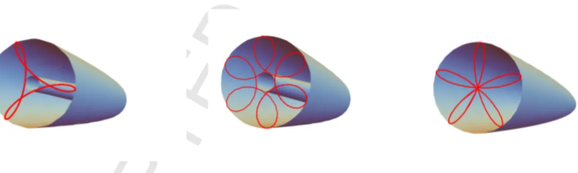
• For γ a rational number with|γ|<1, we already know that (1 +γ)/(1−γ) =p/q is also rational, and we have the motion of the superintegrable FD system with closed trajectories. Some examples of these trajectories, together with the corresponding effective potentials, are shown in Figure 2. When the values of α0 and β0 are equal, the effective potential
given by (4.3) has no singularity because the angular momentumpϕ=|β+(0)|2− |α+(0)|2 is zero. This can be seen in the last graphic of Figure 2. When they have different values, the angular momentum is different from zero and the effective potential has a singularity. This can be appreciated in the first two graphics of Figure 2. The number of the lobes of the trajectories depends on the values of pand q and it is given byp+q, because the fundamental period of the trajectories is given by T = 2π/(p+q) due to (4.14). The number of total turning points for the coordinateρ is 2(p+q).
Figure 2: Three plots of the classical trajectories (4.24) of the classical FD system (in red) with the surfaces of the effective potentials. On the left{γ= 1/3, p+q= 3, `= 96, α0= 10, β0= 14, θ1=θ2= 0},
on the center {γ = 2/3, p+q = 6, ` = 125, α0 = 10, β0 = 15, θ1 = 2, θ2 = 3}, and on the right {γ= 1/5, p+q= 5, `= 0, α0= 12, β0= 12, θ1= 2, θ2= 1}.
4.4
Symmetries of the classical FD system
It is well known that, in general, any constant of motion G(q,p) produce a type of infinitesimal canonical transformations on the phase-space, which lead to transformations of the classical tra-jectories: G(q,p) can be considered as a generator of an infinitesimal canonical transformation, such that any functionu(q,p) is changed as follows
d u
whereηis a continuous parameter. In principle, by integrating equation (4.26), a finite canonical transformation,u(η), is obtained. A formal solution can be found by expandingu(η) in a Taylor series about the initial conditions [33].
For the problem we are studying, it is convenient to start by computing the changes generated by S± and L given by (4.7)-(4.8) on the functions α± and β±, since the canonical variables (x, y, px, py) can be expressed in terms of α± andβ± according to (4.23). We can evaluate the following:
? Infinitesimal action of L:
d α± d η ={α
±,L}=∓iα±, d β±
d η ={β
±,L}=±iβ±. (4.27)
? Infinitesimal action of S+:
d α+
d η =iq(α
−)q−1(β+)p, d α−
d η = 0,
d β+ d η = 0,
d β−
d η =−ip(α
−)q(β+)p−1. (4.28)
? Infinitesimal action of S−:
d α+ d η = 0,
d α−
d η =−iq(α
+)q−1(β−)p, d β+
d η =ip(α
+)q(β−)p−1, d β−
d η = 0. (4.29)
In the sequel we will deal with the three special cases we have already considered in the quantum context: HO, Landau and rational FD systems. We will show that the integration of these differential equations leads to the finite action of symmetry transformations. In the case of the HO and Landau systems such finite transformations are linear and we will find then explicitly. However, in the generic rational FD system we will only be able to find the explicit formulas for some special cases which are essentially nonlinear.
4.4.1 Harmonic oscillator (q=p= 1 or γ= 0)
We introduce the new (real) constants of motion
S1 = (S++S−)/2, S2 = (S+− S−)/2i , S=L/2, (4.30)
in terms of{S±,L}given by (4.7)-(4.8), forq=p= 1. These new constants of motion{S1,S2,S} close the Lie algebrasu(2) [33], with Poisson brakets
{S,S1}=S2, {S,S2}=−S1, {S1,S2}=S. (4.31)
The angular momentum 2S generates rotations of the classical trajectories, while S1 andS2
give a type of transformation changing the shape of the trajectories. The finite transformations for these generators can be obtained by integrating the differential equations (4.27)-(4.29). The results are the following:
? Finite action of S1:
x0=xcosη/2 +pxsinη/2, y0 =ycosη/2−pysinη/2,
p0x=pxcosη/2−xsinη/2, p0y =pycosη/2 +ysinη/2.
? Finite action of S2:
x0=xcosη/2 +pysinη/2, y0=ycosη/2 +pxsinη/2,
p0x=pxcosη/2−ysinη/2, p0y =pycosη/2−xsinη/2.
(4.33)
? Finite action of S:
x0=xcosη/2−ysinη/2, y0=ycosη/2 +xsinη/2,
p0x=pxcosη/2−pysinη/2, p0y =pycosη/2 +pxsinη/2.
(4.34)
The effects of all these transformations (classical symmetries) for different values ofη on the trajectories can be seen in Figure 3. In these plots, the dashed lines correspond to the initial trajectory (η= 0).
The transformations generated byS1andS2leave the Hamiltonian invariant but they change
the value of the angular momentum. This means that, under these transformations, the effective potential changes, but the energy is conserved, and therefore they may be considered as classical analogs of the quantum mechanical shift operators.
-3 -2 -1 1 2 3 x
-3 -2 -1 1 2 3 y
-3 -2 -1 1 2 3 x
-3 -2 -1 1 2
3y
-3 -2 -1 1 2 3 x
-3 -2 -1 1 2 3 y
Figure 3: Plot of the action of the symmetry group elements on the classical trajectories of the harmonic oscillator: on the left they are generated by S (4.34), in the center byS1(4.32), and on the right byS2
(4.33); the relevant parameters are chosen to be{γ= 0, α0= 1, β0= 2, θ1= 0, θ2= 0}.
4.4.2 Landau system (q= 1, p= 0 or γ= 1)
For this case, the constant of motions given by (4.7) take the form
M=α+α−, N =β+β−, S−=β−, S+=β+. (4.35)
We introduce again real constants of motion in terms of S±given by (4.35) and L:
S1 = (S++S−)/2, S2= (S+− S−)/2i , S =L=N − M. (4.36)
They satisfy
{S,S1}=S2, {S,S2}=−S1, {S1,S2}=−1
2. (4.37)
? Finite action of S1:
x0 =x, y0=y+ η
2, p0x=px−
η
2, p0y=py. (4.38)
? Finite action of S2:
x0 =x− η
2, y
0 =y, p0
x=px, p0y =py−η
2. (4.39)
The action of S has the same form as in (4.34).
The effect of all these symmetry transformations for different values of η on the trajectories can be seen in Figure 4. The value η= 0 corresponds to the initial motion, and it is shown in Figure 4 by dashed line.
-1 1 2 3 x
-1 1 2 3 y
0.5 1.0 1.5 2.0 2.5 3.0 x
-1.0 -0.5 0.5 1.0 1.5 y
0.5 1.0 1.5 2.0 2.5 3.0 x
-1.0
-0.5 0.5 1.0 y
Figure 4: Plot of the action of the symmetry group elements on the classical trajectories of the Landau system: on the left they are generated by S (4.34), in the center byS1 (4.38), and on the right by S2
(4.39); the relevant parameters are chosen to be{γ= 1, α0= 1, β0= 2, θ1= 0, θ2= 0}.
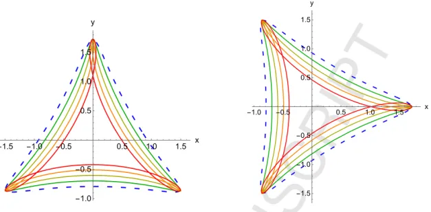
4.4.3 Rational FD system for arbitrary q, p
For the generic rational FD system we consider the constants of motion already introduced in (4.36). Again,S is the angular momentum, and therefore it generates rotations, as described in the HO and Landau subsection. Thus, we will concentrate on the action of S1 andS2.
(A) Finite action of S1: we have to solve the following nonlinear equations:
d α+
d η =i q
2(α−)
q−1(β+)p, d α−
d η =−i q
2(α
+)q−1(β−)p,
d β+
d η =i p
2(α
+)q(β−)p−1, d β−
d η =−i p
2(α−)
q(β+)p−1.
(4.40)
It is quite difficult to find the general solution ofα±andβ±for any value ofq andp, but it is possible to get some special solutions. Let us propose the following polar-type ansatz for the solutions of (4.40)
α±(η) =ρ1(η)e±iθ1(η), β±(η) =ρ2(η)e±iθ2(η), (4.41)
whereρ1, ρ2andθ1, θ2are real functions depending on the group parameterη. Substituting
in (4.40), we arrive to the following equations
d ρ2
d η =− p
2ρ q
1ρp2−1 sin(qθ1−pθ2), d θ2
d η = p
2ρ q
1ρp2−2 cos(qθ1−pθ2),
d ρ1
d η = q
2ρ q−1
1 ρp2 sin(qθ1−pθ2),
d θ1
d η = q
2ρ q−2
1 ρp2 cos(qθ1−pθ2).
They lead to energy conservation for the classical FD system: pρ2
1+qρ22 =c1 = ε. Now,
let us consider two special cases:
(A1) Ifqθ1−pθ2 = 0, then from (4.42) it follows that ρ1 and ρ2 are constants satisfying
ρ1/ρ2=q/pandθ1 andθ2 are linear functions of ηgiven by
θ1(η) = q
2ρ q−2
1 ρp2η+φ1, θ2(η) = p
2ρ q
1ρp2−2η+φ2, (4.43)
where the constants φ1, φ2 also satisfyφ1/φ2 =p/q. In summary, we have integrated the
action of the symmetry on the points characterized byα±=ρ1e±iφ1, β±=ρ2e±iφ2, such
that ρ1/ρ2 = q/p and φ1/φ2 = p/q. It can be shown that this kind of transformations
acting on these points give the same trajectory as their corresponding motion.
(A2) Ifqθ1−pθ2=π/2, thenθ1 andθ2 are constants and ρ1 andρ2 are the functions of
η. For example, we can obtain the explicit expressions ifq= 1 andp= 2:
ρ1(η) =
r
c1
2 tanh r
c1
2 η+c2
, ρ2(η) =√c1sech
r
c1
2 η+c2
, (4.44)
where c1 and c2 are integration constants. Then, we can expressα± andβ± in terms of
the transformation parameterη as:
α±(η) = r c1 2 tanh r c1
2 η+c2
e±iθ1, β±(η) =√c
1sech
r
c1
2 η+c2
e±iθ2. (4.45)
Finally, we express the finite action ofS1 as:
x0=√c1sech
r
c1
2 η+c2
cosθ2+
r
c1
2 tanh r
c1
2 η+c2
cos2θ2+
π
2
,
y0 =√c1sech
r
c1
2 η+c2
sinθ2−
r
c1
2 tanh r
c1
2 η+c2
sin2θ2+ π
2
,
p0x=−√c1sech
r
c1
2 η+c2
sinθ2−
r
c1
2 tanh r
c1
2 η+c2
sin2θ2+
π
2
,
p0
y=√c1sech
r
c1
2 η+c2
cosθ2−
r
c1
2 tanh r
c1
2 η+c2
cos2θ2+π
2
.
(4.46)
In Figure 5 (left), we represent some examples of motions which are related by means of this finite action of the symmetry S1. The initial points α±(0) and β±(0) are fixed by
(4.44) with η= 0, andqθ1−pθ2 =π/2. Case (A2) is more interesting than (A1) because
these symmetry transformations connect different motions.
(B) Finite action of S2 = (S+− S−)/2i. The differential equations to be solved are:
d α+
d η = q
2(α−)
q−1(β+)p, d α−
d η = q
2(α
+)q−1(β−)p,
d β+
d η =− p
2(α
+)q(β−)p−1, d β−
d η =− p
2(α−)
q(β+)p−1,
(4.47)
which have the same difficulties as the symmetryS1. Nevertheless, we can find particular
solutions corresponding to the two cases (A1) and (A2) considered above forS1. They are
-1.5 -1.0 -0.5 0.5 1.0 1.5 x
-1.0 -0.5 0.5 1.0 1.5 y
-1.0 -0.5 0.5 1.0 1.5 x
-1.5
-1.0
-0.5 0.5 1.0 1.5 y
Figure 5: Different motions connected by the symmetries generated by S1 (left) and by S2 (right)
corresponding to the energy ε= 2 andγ= 1/3, q= 1, p= 2, c2 = 0.5, θ2 = π/8. The initial motion is
represented by the dotted blue curve.
5
Coherent states
It was shown in Section 2.2 that the quantum FD system has two independent sets of ladder operatorsa±andb±, which generate all the eigenfunctions from the ground state. Therefore, it is quite natural to define the coherent states for this system as the eigenstates of both annihilation operators a− andb−:
a−|α, βi=α|α, βi, b−|α, βi=β|α, βi, (5.1)
whereα, β ∈C. As both type of operators commute, we can write|α, βi=|αi ⊗ |βi, being |αi
and|βicoherent states of the usual harmonic oscillator. Therefore, we can write|α, βias
|α, βi= e−|α|2/2
∞ X
m=0
αm
√
m!|mi !
⊗ e−|β|2/2
∞ X
n=0
βn
√
n!|ni !
. (5.2)
Now, we are interested in an explicit form for the coherent state wavefunction analytically by substituting the differential realizations (2.14)-(2.15) of the annihilation operators a−, b− in (5.1):
Ψα β(ρ, ϕ) =K(α, β)ρ1/2e−ρ
2/2
eρ(α e−i ϕ+β ei ϕ), (5.3)
where K(α, β) is a normalization constant that must be determined because it will play an essential role later. The probability density is
|Ψα β(ρ, ϕ)|2=|K(α, β)|2ρ e−ρ
2
e2ρ u(α ,β) cos (ϕ−ϕ0), (5.4)
whereu(α , β) =|α+β∗|. After imposing normalization of the coherent state Z
R2|Ψα β(ρ, ϕ)|
2 dρ dϕ= 1,
|K(α, β)|2 can be expressed in terms ofu(α , β) and the modified Bessel functionsI1, I0 as
|K(α, β)|2= 2
π3/2eu2/2
(u2I
1(u2/2) + (u2+ 1)I0(u2/2))
The time evolution of the eigenstates |mi ⊗ |niof the FD Hamiltonian is
e−itH|mi ⊗ |ni=e−itεmn|mi ⊗ |ni, (5.6)
and taking into account the eigenvalue equation for the FD system HΨm,n =εm,nΨm,n, with
εm,n=m(1 +γ) +n(1−γ) + 1, we can write the time evolution of |α, βi:
|α, β, ti = e−i t e−|α|2/2
∞ X
m=0
(α e−i(1+γ)t)m
√
m! |mi !
⊗ e−|β|2/2
∞ X
n=0
(β e−i(1−γ)t)n
√
n! |ni !
= e−i t|α e−i(1+γ)t, β e−i(1−γ)ti. (5.7)
This result means that the time evolution of the coherent state wavefunction (5.3) can be obtained replacing α→α e−i(1+γ)t andβ→β e−i(1−γ)t. In order to find the correspondence of classical trajectories and coherent states, we should identify the eigenvalues α, β in (5.1) with the valuesα− andβ− of (4.20).
In Figure 6, we plot the probability density of some coherent states and the analogous classical trajectories, which were already considered in Figure 2. From the analysis of both figures it can be seen that the classical trajectories and the expected value of the position coordinates (x, y) for the coherent states are very close.
Figure 6: Plot of the probability density (5.4) of the coherent states and the classical trajectories (red) for: {γ= 1/3, α0= 10, β0= 14, θ1=θ2= 0}(left),{γ= 2/3, α0= 10, β0= 15, θ1= 2, θ2= 3} (center)
and {γ= 1/5, α0= 12, β0= 12, θ1= 2, θ2= 1}(right).
6
Conclusions and remarks
In this work, we have systematically studied the symmetry properties of the FD system, which is characterized by a parameter γ relating the frequencies associated to the harmonic oscillator (ωo) and the magnetic field (ωc). We took a different approach from the existing literature, paying attention to the similarities of symmetries in the quantum and classical frameworks: the connection of symmetries and degeneracies in the quantum context and the relation between constants of motion and transformation of motions with the same energy in the classical case.
can also be expressed in terms of a±, b±. However, only when γ is rational the FD system is superintegrable.
In the particular casesγ= 0 (harmonic oscillator, HO) andγ =±1 (Landau), the symmetries are of second order and allow separation in other coordinate systems (besides polar). In these two cases, the symmetry operators close Lie algebras: u(2) for HO andos(1)⊕u(1) for Landau. However, in the other superintegrable rational cases the symmetries are of higher order and the separation is only possible in polar coordinates. For such cases the symmetry algebras are polynomial, and its explicit form was computed.
We have also explained the relation between the symmetries and degeneracy of the energy levels. The symmetry operators acting on any eigenfunction will generate the whole energy eigenspace. For the HO the dimension of each eigenspace is k+ 1 (k = 0,1, . . .), for Landau it is infinite dimensional, and for the FD system is k+ 1, where the number of eigenspaces with the same degeneracy dimension is p×q.
In the classical FD system, there are ladder functions α± and β± corresponding to the quantum operatorsa± andb±. Following the same procedure as in the quantum case, we have shown that the FD system corresponding to rational γ values is superintegrable. We have computed explicitly the Poisson algebra of constants of motion, which are the classical limit of the corresponding quantum symmetry algebra.
The classical trajectories are directly obtained from the constants of motion. Due to the superintegrability they are closed, and in this case we have also seen that they are 2π/(p+q) periodic in the polar angle ϕ and they have 2(p+q) turning points in the variable ρ. We have studied the action of the constants of motion as generators of symmetry transformations of the classical motion. In particular, we have been able to give explicit expressions of the finite action for the HO and Landau. In the general rational FD case the differential equations are nonlinear and a full integration is quite difficult. However, we have been able to find solutions for some particular cases, showing how some motions are transformed by means of finite symmetry transformations.
The connection between the quantum and classical systems is established through coherent states: we have computed explicit expressions of the coherent states in polar coordinates and we have shown that their evolution follow closely the classical motion trajectories.
In this work, we have restricted to the simplest original FD system, but there are other models where our considerations also apply. For instance, quantum dots with anisotropic oscillator confining potentials have been already considered in the literature [5, 8]. The superintegrability conditions can be extended in this case for another characteristic frequency quotient (playing the role of γ), however the separable coordinates are not polar, but elliptic. In the context of paraxial optics, more interaction terms appear in the Hamiltonian allowing for a discussion of the conditions to implement superintegrability. Similar properties have been displayed in some graphics of the coherent states and classical trajectories [24, 25]. Other variations of the FD model are related with spin Zeeman and Rashba effects, or with the inclusion of electric fields [8]. Works in these directions are presently in progress.
Acknowledgments
References
[1] V. Fock. Bemerkung zur quantelung des harmonischen oszillators im magnetfeld.Zeitschrift
f¨ur Physik, 47:446–448, 1928.
[2] C.G. Darwin. The diamagnetism of the free electron. Math. Proc. Cambridge Philos. Soc., 27:86–98, 1931.
[3] P. Hawrylak. Single-electron capacitance spectroscopy of few-electron artificial atoms in a magnetic field: Theory and experiment. Phys. Rev. Lett., 71:3347–3350, 1993.
[4] L.P. Kouwenhoven, D.G. Austing, and S. Tarucha. Few-electron quantum dots. Rep. Prog.
Phys., 64:701–736, 2001.
[5] A.V. Madhav and T. Chakraborty. Electronic properties of anisotropic quantum dots in a magnetic field. Phys. Rev. B, 49:8163–8168, 1994.
[6] H.-Y. Chen, V. Apalkov, and T. Chakraborty. Fock-darwin states of dirac electrons in graphene-based artificial atoms. Phys. Rev. Lett., 98:186803, 2007.
[7] B. Szafran, F.M. Peeters, S. Bednarek, and J. Adamowski. Anisotropic quantum dots: Correspondence between quantum and classical wigner molecules, parity symmetry, and broken-symmetry states. Phys. Rev. B, 69:125344, 2004.
[8] S. Avetisyan, P. Pietil¨ainen, and T. Chakraborty. Strong enhancement of rashba spin-orbit coupling with increasing anisotropy in the fock-darwin states of a quantum dot. Phys. Rev. B, 85:153301, 2012.
[9] B.L. Johnson and G. Kirczenow. Enhanced dynamical symmetries and quantum degenera-cies in mesoscopic quantum dots: Role of the symmetries of closed classical orbits.Europhys.
Lett., 51:367–373, 2000.
[10] J.M. Lauch and E.L. Hill. On the problem of degeneracy in quantum mechanics. Phys. Rev., 40:641–645, 1957.
[11] M. Moshinsky, J. Patera, and P. Winternitz. Canonical transformation and accidental degeneracy. iii. a unified approach to the problem. J. Math. Phys., 16:82–92, 1975.
[12] M. Moshinsky and C. Quesne. Does accidental degeneracy imly a symmetry group? Ann.
Phys., 148:462–488, 1983.
[13] M. Moshinsky, N. M´endez, E. Murow, and J.W.B. Hughes. Accidental degeneracies in the zeeman effect and the symmetry groups. Ann. Phys., 155:231–268, 1984.
[14] C. Quesne. Accidental degeneracies and symmetry group of the harmonic oscillator in a strong magnetic field. J. Phys. A: Math. Gen., 19:1127–1139, 1986.
[15] W. Miller, S. Post, and P. Winternitz. Classical and quantum superintegrability with applications. J. Phys. A: Math. Theor., 46:423001, 2013.
[16] E.G. Kalnins, W. Miller, and G.S. Pogosyan. Superintegrability and higher-order constants for classical and quantum systems. Phys. Atom. Nucl., 74:914–918, 2011.
[18] I.A. Malkin and V.I. Man’ko. Coherent states of a charged particle in a magnetic field. Sov.
Phys. JETP, 28:527–532, 1969.
[19] I.A. Malkin and V.I. Man’ko. Coherent states and green’s function of a charged particle in variable electric and magnetic fields. Sov. Phys. JETP, 32:949–953, 1971.
[20] A. Feldman and A.H. Kahn. Landau diamagnetism from the coherent states of an electron in a uniform magnetic field. Phys. Rev. B, 28:4584–4589, 1970.
[21] I.W. Sudiarta and D.J.W. Geldart. Solving the schr¨odinger equation for a charged particle in a magnetic field using the finite difference time domain method.Phys. Lett. A, 372:3145– 3148, 2008.
[22] H.E. Santos, N.M.R. Peres, and J.M.B. Lopes dos Santos. Evolution of squeezed states under the fock-darwin hamiltonian. Phys. Lett. A, 80:053401, 2009.
[23] A. Dehghani and B. Mojaveri. New physics in landau levels. J. Phys. A: Math. Theor., 46:385303, 2013.
[24] Y.F. Chen, Y.C. Lin, K.F. Huang, and T.H. Lu. Spatial transformation of coherent optical waves with orbital morphologies. Phys. Rev. A, 82:043801, 2010.
[25] Y.F. Chen. Geometry of classical periodic orbits and quantum coherent states in coupled oscillators with su(2) transformations. Phys. Rev. A, 83:032124, 2011.
[26] E. Drigho-Filho and M.A.C. Ribeiro. Generalized ladder operators for shape-invariant potentials. Phys. Scrip., 64:386–412, 2001.
[27] D.J. Fern´andez, J. Negro, and M.A. del Olmo. Group approach to the factorization of the radial oscillator equation. Ann. Phys., 252:386–412, 1996.
[28] K. Kikoin, M. Kiselev, and Y. Avishai.Dynamical Symmetries for Nanostructures. Springer-Verlag/Wien, 2012.
[29] S¸. Kuru and J. Negro. Factorizations of one dimensional classical systems. Ann. Phys., 323:413–431, 2008.
[30] L.M. Nieto. Coherent and supercoherent states with some recent applications. AIP Conf.
Proc., 809:3–23, 2006.
[31] S. Cruz y Cruz, S¸. Kuru, and J. Negro. Classical motion and coherent states for p¨oschl-teller potentials. Phys. Lett. A, 372:1391–1405, 2008.
[32] R. Campoamor-Stursberg, M. Gadella, S¸. Kuru, and J. Negro. Action-angle variables, ladder operators and coherent states. Phys. Lett. A, 376:2515–2521, 2008.