A Self-Adaptive Evolutionary Approach to the
Evolution of Aesthetic Maps for a RTS Game
Ra´
ul Lara-Cabrera, Carlos Cotta and Antonio J. Fern´
andez-Leiva
∗Universidad de M´
alaga, Andaluc´ıa Tech, Departamento de
Lenguajes y Ciencias de la Computacin.
Abstract
Procedural content generation (PCG) is a research field on the rise, with numerous papers devoted to this topic. This paper presents a PCG method based on a self-adaptive evolution strategy for the automatic gen-eration of maps for the real-time strategy (RTS) game Planet Wars. These maps are generated in order to fulfill the aesthetic preferences of the user, as implied by her assessment of a collection of maps used as training set. A topological approach is used for the characterization of the maps and their subsequent evaluation: the sphere-of-influence graph (SIG) of each map is built, several graph-theoretic measures are computed on it, and a feature selection method is utilized to determine adequate subsets of measures to capture the class of the map. A multiobjective evolutionary algorithm is subsequently employed to evolve maps, using these feature sets in order to measure distance to good (aesthetic) and bad (non-aesthetic) maps in the training set. The so-obtained results are visually analyzed and compared to the target maps using a Kohonen network.
1
Introduction
Within the field of computational intelligence we find the procedural content generation (PCG) [1] for games, which represents a set of algorithmic techniques used to automatically generate game content, whether it be maps, levels, 3D models, music and/or even rules. The employment of PCG provides several ad-vantages to the development of video games, such as a reduction in the expenses linked to manually creating the content, a reduced amount of used memory and the ability to create infinite games (e.g., new levels/characters/missions can be automatically created to extend the lifetime of the game). PCG has been ap-plied adequately during the development of several successful commercial games such as Borderlands saga or the sandbox games Minecraft and Terraria.
PCG covers various methodologies, being our work focused on the search-based procedural content generation (SBPCG) [2]. This search-search-based method-ology consists in generating a substantial amount of game resources in order to find, through a guided search (e.g., via meta-heuristics) those assets that
∗Email: {
meet a certain level of quality. Therefore, it is necessary to define the quality criterion for the generated content. The quality criteria we used in this study was how aesthetic the generated resources were (more specifically, the content we consider are maps for a real-time strategy game). In our earlier work [3, 4], we used two different criteria when generating and evaluating the maps, in
particular balance (i.e., no player gets an advantage over the other) and level
of dynamism (measured in terms of resource fluctuations or by evaluating the nature of confrontations between the players). The goal in both cases was to produce interesting games providing atractive challenges to the players. While fulfilling our requirements of balance and dynamism, the generated maps lacked aesthetic (for example, maps with their planets clustered in a small region), an interesting property that a map might has and that may conduct to obtain even more appealing games; for this reason, we now analyze how to incoporate this feature to our generated maps.
The chosen game,Planet Wars, is a real-time strategy game developed in
the context of the Google AI Challenge competition. This game genre offers a wide variety of artificial intelligence research problems [5] (such as opponent modelling, spatial and temporal reasoning, resource management and real-time planning). Planet Wars is a game about conquering planets and fighting space battles between several players. The goal is to conquer all the planets while trying to eliminate all opponents. These planets, which can hosts ships and are distributed over a 2-dimensional plane, may belong to any player or be neutral (that is, the planet belongs to nobody). Non-neutral maps produce new ships every turn, depending on their size. Players send groups of ships (i.e., fleets) from planets they control to other ones. If the player owns the target planet then the number of arriving ships is added to the number of defending ships on that planet, otherwise a battle takes place in the target planet: ships of both sides destroy each other so the player with the highest number of ships owns the planet (with a number of ships determined by the difference between the initial number of ships). The distance between the planets affects the required time for a fleet to arrive to her destination, which remains fixed during the fleet movement (that is, it is not possible to change the destination of a moving fleet). Although the game is played in turns, players issue their orders at the same time, so it can be considered as a real-time game. Games can end when a player has defeated the other or when the maximum number of turns is reached (the winner is the player with the highest number of controlled planets).
2
Background
pro-gramming), using either subjective human-based feedback [8, 9] or automated quality measures such as accessibility [10] or edge-length [11]. Another example by Mahlmann et al. [12], who suggested a search-based map generator based on the transformation of low resolution matrices into higher resolution maps (using
cellular automatas) for a simplified version of the RTS game Dune II.
3
Map Characterization
The maps from Planet Wars are made of a certain number of planets np
dis-tributed over a 2D plane. Every planet is defined by their position on the plane
(coordinates (xi, yi)), their sizesi and a number of shipswi. The size si sets
the rate at which a planet will generate new ships every turn (as long as the
planet is controlled by any player) while the remaining parameter,wi, indicates
the number of defending ships. We denoted a map as a list [~ρ1, ~ρ2,· · · , ~ρnp],
where each ~ρi is a tuple hxi, yi, si, wii. It is mandatory to specify the initial
home planets of the players, which were fixed as the first two planets ~ρ1 and
~
ρ2. The number of planets np is not fixed and should range between 15 and
30 as set by the rules of the Google AI Challenge 2010 (this variable number
of planets is included in the self-adaptive evolutionary approach described later on).
We characterized every map by computing several measures from the map’s spheres-of-influence graph (SIG) [13]. This kind of graph can be used to extract information about a set of points and establishes a relationship between them, which is based on their spatial arrangement and is not affected by rotation, translation and scaling (see Figure 1). SIGs can be applied to many research areas and applications, such as in computer vision (as a low-level operator for object recognition from input dot patterns), data mining (for clustering objects with similar attribute values) and computer graphics (for defining surfaces over point clouds). The procedure for generating the SIG for a certain map is as follows:
1. For each planetpiplaced at (xi, yi), compute the distancedito the closest
planet
di= min
j {k(xi−xj, yi−yj)k |j 6=i} (1)
wherekvkis the Euclidean norm of vectorv.
2. For each planet pi, draw a circle with center (xi, yi) and radiusdi
3. Build the SIG as a graphG(V, E), whereV ={p1,· · · , pnp}and (u, v)∈E
iff the circles with centers inuand vintersect.
We gathered two sets of maps, which were used later as a baseline to compare with, one of them containing 100 maps with good aesthetics and the other one including 100 non-aesthetic maps. An expert evaluated the maps and tagged them as aesthetic or non-aesthetic, based on her perceptions and artistic criteria. Then we computed several measures relating to the previously generated SIGs, namely:
• Number of connected components (sub-graphs in which any two vertices
Figure 1: A sphere-of-influence graph.
Density 0.120.140.16
0.180.200.220.240.26
Size/Betw. correlation 0.60.4
0.20.0 0.20.4
Neigh. size assort. 0.3 0.2 0.1 0.0 0.1 0.2
(a)
Density 0.120.140.16
0.180.200.220.240.26 0.20.30.4Clustering 0.50.6
0.70.8 Size/Degr. correlation 0.80.6
0.4 0.2 0.00.2 0.4 0.6
(b)
Figure 2: Distribution of aesthetic (circles) and non-aesthetic (crosses) maps according to the values of the variables from group A (a) and B (b)
• Average node’s degree (number of edges incident to the node).
• Density of the graph, which measures the ratio between number of edges
and nodes (specifically for undirected graphsδ= 2m/(n(n−1)), with n
andmbeing the number of nodes (i.e. np) and edges respectively).
• Average clustering coefficient. The clustering coefficientciof a node
quan-tifies how interconnected (or grouped) with his neighbors it is.
Mathemat-ically, ci = 2Ei/[ki(ki−1)] where Ei is the number of edges connecting
the immediate neighbors of nodeiandki is the degree of nodei.
• Pearson correlation between the size of the nodes and their betweenness.
The latter is a measure of the importance as intermediate gateway of a node in a graph, as is computed as the average fraction of shortest paths between any two nodes that go through a third certain node.
• Size assortativity, i.e., Pearson correlation coefficient between the size of nodes connected in the graph.
Subsequently, we created a Random Forest classifier for each possible combi-nation of the above measures and we evaluated the performance of the classifiers by a Leave-one-out (LOO) cross-validation. Each classifier had 50 estimators (i.e., decision trees), bootstrap sampling and the Gini impurity criterion as the function to measure the quality of the splits. After analyzing the AUC (Area under ROC curve) values of the different combinations, we decided to use the following groups of variables as the map characterization (see Figure 2):
• Group A: Graph’s density (δ), correlation between node size and
be-tweenness (ρSB), and size assortativity (ρSize) (i.e., Pearson correlation
coefficient between the size of connected planets). (AU C= 0.9916)
• Group B: Graph’s density (δ), clustering coefficient (ci) and Pearson’s
correlation coefficient between planets’ sizes and their degree (ρSG). (AU C=
0.9984)
We compared the similarity between maps using these two groups of features
in the following way: each map is characterized by a tuple hδ, ρSB, ρSizei and
hδ,c¯i, ρSGi; then the Euclidean distance between these tuples defined the
similar-ity among the planets they represented. The previously defined sets of aesthetic and non-aesthetic maps made up a baseline to compare with so the problem of generating aesthetic maps turned into an optimization problem about min-imizing the distance between generated and aesthetics maps while maxmin-imizing their distance to non-aesthetic maps. The latter was essential in order to insert diversity into the set of generated maps, hence avoiding the creation of maps that were very similar to the aesthetic ones.
4
Procedural Map Generation
We used a NSGA-II multi-objective self-adaptive (µ+λ) evolution strategy (with
µ= 10 andλ= 100) as the map generator. The objectives, as described in
sec-tion 3, were to increase and reduce the distance between the generated maps and non-aesthetic and aesthetic maps, respectively. The solutions are represented as
mixed real-integer vectors of planets, planet’s coordinates (xi, yi) are real-valued
numbers but sizes si and initial number of ships wi are positive integers. To
overcome this situation we considered a hybrid mutation operator with different methods for parameters of either type. For real-valued parameters, it used a Gaussian mutation; as for integer variables, it used a method that generates suitable mutations [14, 15].
The method for integer variables is similar to the mutation of real values but, in this case, the difference of two geometrically distributed random ables produces the perturbation (instead of the normal distributed random
vari-ables used by the Gaussian mutation). Real-valued parametershr1, ..., rniwere
extended with nstep sizes, one for each parameter (thus providing the means
for self-adaptation), resulting in hr1, ..., rn, σ1, ..., σni. The mutation method is
specified as follows:
σ0i = σi·eτ
0·N(0,1)+τ·N
i(0,1) (2)
0.1 0.2 0.3 0.4 0.5 0.6 0.7
0.2 0.4 0.6
distance to aesthetics
distance to non−aesthetics
Aesthetics
Non−aesthetics
Non−dominated
(a)
0.2 0.4 0.6 0.8
0.2 0.4 0.6
distance to aesthetics
distance to non−aesthetics
Aesthetics
Non−aesthetics
Non−dominated
(b)
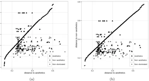
Figure 3: Cumulative set of non-dominated generated solutions (circle) for group of variables A (a) and B (b) and maps from aesthetic (triangle) and non-aesthetic (square) baseline sets.
whereτ0∝1/√2n, andτ∝1/p2√n. A boundary rule is applied to step-sizes
to forbid standard deviations very close to zero: σi0 < 0 ⇒ σ0i = 0 (in this
algorithm,σ0 comprises a 1% of the parameter’s range).
Regarding integer-valued parameters hz1, ..., zmi they were extended in a
similar way as real-valued parameters, resulting in hz1, ..., zm, ς1, ..., ςmi. The
following equations define the mutation mechanism:
ςi0 = max(1, ςi·eτ·N(0,1)+τ
0
·N(0,1)) (4)
ψi = 1−(ςi0/m)
1 + s
1 +
ςi0 m
2
−1
(5)
zi0 = zi+
ln(1
−U(0,1))
ln(1−ψi)
−
ln(1
−U(0,1))
ln(1−ψi)
(6)
whereτ = 1/√2m andτ0= 1/p2√m.
In the case of the recombination, we chose a “cut and splice” operator that recombines two individuals by swapping cut pieces with different sizes. It selects one cut point for each individual and then swaps these pieces, getting two new individuals with a different number of planets in relation to their parents (af-fecting the complexity of the maps, i.e., the number of planets in the solutions, and enabling the algorithm with additional self-adaptation features).
Assort. Sizes Corr. Size−Betw. Density
0.0 0.4 0.8
Aesthetic maps
Assort. Sizes Corr. Size−Betw. Density
0.0 0.4 0.8
Non−dominated maps
Assort. Sizes Corr. Size−Betw. Density
0.0 0.4 0.8
Non−Aesthetic maps
(a)
Clustering Corr. Size−Grade Density
0.0 0.4 0.8
Aesthetic maps
Clustering Corr. Size−Grade. Density
0.0 0.4 0.8
Non−dominated maps
Clustering Corr. Size−Grade Density
0.0 0.4 0.8
Non−Aesthetic maps
(b)
Figure 4: Distribution of the variables from each group, group A (a) and group B(b), for both non-dominated solutions and baseline maps.
5
Experimental Results
We conducted two sets of experiments, one for each group of variables. Each set of experiments consisted of 20 runs of the evolutionary algorithm described previously, with 100 generations per run, obtaining a set of non-dominated solutions in each. Then we calculated the cumulative set of non-dominated solutions for each group (see Figure 3). As we can see, the relationship between both distances is linear regardless of the group of variables used, specifically in the middle range of the Pareto front. This suggests that it is hard to increase the distance of the solutions to non-aesthetic maps without also increasing it toward the aesthetic maps, in addition to the high density of the search space. Furthermore, we should observe that there are aesthetic maps from the baseline with a higher mean difference to non-aesthetics maps than some non-aesthetic ones, and vice versa (i.e., there are aesthetic maps that are more similar to non-aesthetic maps than other non-aesthetic ones, and vice versa). This hints at the subjectivity of the expert during the process of map classification.
Regarding how the characterization values of baseline and generated maps are distributed (see Figure 4), we can observe that there are not high differences between the variables from aesthetic and non-aesthetic maps. However, some
values from non-dominated maps, such as ρSB and ρSize from group A, are
higher than their corresponding values from baseline maps, which should explain the high distance between some of the non-dominated solutions and baseline maps (as seen in Figure 3).
We created two self-organizing maps (SOMs), one for each group of vari-ables, so that we could be sure about the validity of the generated maps and we could make a comparison between both groups of variables. These maps are artificial neural networks that are trained using unsupervised learning to gen-erate a discretized representation of the input space [16]. In this case, we built
(a) (b)
Figure 5: Map’s distribution over the SOMs (groups A (a) and B (b)). Red for non-aesthetic, green for aesthetic and blue for non-dominated.
using our baseline maps as the training set, and then, we projected the non-dominated solutions onto the SOM (see Figure 5). As we can see in both cases, they were not able to establish a clear distinction between aesthetic (green) and non-aesthetic (red) maps (note the overlapped zones). Regarding the projected solutions, they occupy a distinct region in the case of group A, while in group B the region is blurred (even some solutions are located in a different area: specifically the lower right area). Besides, the red component of the solutions from group B seems to be greater than the group A red component, which may indicate that the results obtained from the group B variables are lower quality.
6
Conclusion
● ● ● ● ● ● ● ● ● ● ● ● ● ● ● ● ● ● ● ● ● ● ● 41 101 101 43 43 79 79 55 55 40 40 58 58 67 67 63 63 4 4 63 63 63 63 (a) ● ●● ● ● ● ● ● ● ● ● ● ● ● ●
101 2 2 2 2 101 101 101 2 2 2 101 101 101 2 (b) ● ● ● ● ● ● ● ● ● ● ● ● ● ● ● ● ● ● ● ● ● ● ● 4 5 3 8 14 15 15 3 14 2 4 11 6 11 7 7 11 9 2 9 12 12 4 (c) ● ● ● ● ● ● ● ● ● ● ● ● ● ● ●● ● ● ● 5 7 8 9 10 11 4 1 11 10 12 8 4 16
53 1
5 9 (d) ● ● ● ● ● ● ● ● ● ● ● ● ● ● ● ● ● ● ● ● ● ● 15 2 12 12 7 4 7 7 2 12 6 7 8 1 14 2 14 64 14 2 14 29 (e) ● ● ● ● ● ● ● ● ● ● ● ● ● ● ● ● ● ● 6 1 13 3 5 6 8 1 11 6 7 9 5 13 4 8 5 7 (f)
is capable of generating fully playable aesthetic maps for the aforementioned real-time strategy game.
Future work will try to explore the connection between aesthetics and playa-bility (as defined in [3, 4]), defining augmented fitness functions to take the latter into accout. We also plan to introduce the user in the loop in order to refine the automated aesthetic criterion.
Acknoledgements
This work is partially supported by Spanish MICINN under project ANY-SELF (TIN2011-28627-C04-01), Junta de Andaluc´ıa under project
P10-TIC-6083 (DNEMESIS) and Universidad de M´alaga. Campus de Excelencia
Inter-nacional Andaluc´ıa Tech.
References
[1] M. Hendrikx, S. Meijer, J. Van Der Velden, and A. Iosup, “Procedural
content generation for games: A survey,” ACM Trans. Multimedia
Comput. Commun. Appl., vol. 9, no. 1, pp. 1:1–1:22, Feb. 2013. [Online]. Available: http://doi.acm.org/10.1145/2422956.2422957
[2] J. Togelius, G. N. Yannakakis, K. O. Stanley, and C. Browne, “Search-based
procedural content generation: A taxonomy and survey,” IEEE
Transac-tions on Computational Intelligence and AI in Games, vol. 3, no. 3, pp. 172–186, 2011.
[3] R. Lara-Cabrera, C. Cotta, and A. J. Fern´andez-Leiva, “Procedural map
generation for a RTS game,” in13th International GAME-ON Conference
on Intelligent Games and Simulation, A. F. Leiva et al., Eds. Malaga (Spain): Eurosis, 2012, pp. 53–58.
[4] ——, “A procedural balanced map generator with self-adaptive complexity
for the real-time strategy game planet wars,” in Applications of
Evolu-tionary Computation, A. Esparcia-Alc´azaret al., Eds. Berlin Heidelberg: Springer-Verlag, 2013, pp. 274–283.
[5] M. Buro, “RTS games and real-time AI research,” inBehavior
Represen-tation in Modeling and Simulation Conference, vol. 1. Curran Associates, Inc., 2004.
[6] R. Lara-Cabrera, C. Cotta, and A. J. Fern´andez-Leiva, “A Review of
Com-putational Intelligence in RTS Games,” in2013 IEEE Symposium on
Foun-dations of Computational Intelligence, M. Ojeda, C. Cotta, and L. Franco, Eds., 2013, pp. 114–121.
[7] J. Togelius, R. De Nardi, and S. Lucas, “Towards automatic
person-alised content creation for racing games,” in Computational Intelligence
and Games, 2007. CIG 2007. IEEE Symposium on, 2007, pp. 252–259. [8] M. Frade, F. F. de Vega, and C. Cotta, “Modelling video games’ landscapes
users’ experience,” inApplications of Evolutionary Computing, ser. Lecture
Notes in Computer Science, M. Giacobini et al., Eds., vol. 4974. Berlin
Heidelberg: Springer-Verlag, 2008, pp. 485–490.
[9] ——, “Breeding terrains with genetic terrain programming: The evolution
of terrain generators,”International Journal of Computer Games
Technol-ogy, vol. 2009, 2009.
[10] M. Frade, F. de Vega, and C. Cotta, “Evolution of artificial terrains for
video games based on accessibility,” inApplications of Evolutionary
Com-putation, ser. Lecture Notes in Computer Science, C. Di Chio et al., Eds. Berlin Heidelberg: Springer-Verlag, 2010, vol. 6024, pp. 90–99.
[11] M. Frade, F. F. de Vega, and C. Cotta, “Evolution of artificial terrains
for video games based on obstacles edge length,” in IEEE Congress on
Evolutionary Computation. IEEE, 2010, pp. 1–8.
[12] T. Mahlmann, J. Togelius, and G. N. Yannakakis, “Spicing up map
gen-eration,” inApplications of Evolutionary Computation, ser. Lecture Notes
in Computer Science, C. D. Chio et al., Eds., vol. 7248. M´alaga, Spain:
Springer-Verlag, 2012, pp. 224–233.
[13] G. T. Toussaint, “A graph-theoretic primal sketch,” Computational
Mor-phology, pp. 229–260, 1988.
[14] R. Li, “Mixed-integer evolution strategies for parameter optimization and their applications to medical image analysis,” Ph.D. dissertation, Leiden University, 2009.
[15] G. Rudolph, “An evolutionary algorithm for integer programming,” in
Par-allel Problem Solving from Nature III, ser. Lecture Notes in Computer
Sci-ence, Y. Davidor, H.-P. Schwefel, and R. M¨anner, Eds. Jerusalem, Israel:
Springer-Verlag, 1994, vol. 866, pp. 139–148.
[16] T. Kohonen, “The self-organizing map,”Proceedings of the IEEE, vol. 78,