Transmitter-Side Antennas Correlation in
SVD-Assisted MIMO Systems
Andreas Ahrens1, Francisco Cano-Broncano2and C´esar Benavente-Peces2
1 Hochschule Wismar, University of Technology, Business and Design
Department of Electrical Engineering and Computer Science Communications Signal Processing Group
Philipp-M¨uller-Straße 14, 23966 Wismar Germany
andreas.ahrens@hs-wismar.de http://www.hs-wismar.de 2 Universidad Polit´ecnica de Madrid
E.U.I.T de Telecomunicaci´on Ctra. Valencia. km. 7, 28031 Madrid, Spain
fcbroncano@gpss.euitt.upm.es cesar.benavente@upm.es
http://www.upm.es
Abstract. MIMO techniques allow increasing wireless channel perfor-mance by decreasing the BER and increasing the channel throughput and in consequence are included in current mobile communication standards. MIMO techniques are based on benefiting the existence of multipath in wireless communications and the application of appropriate signal pro-cessing techniques. The singular value decomposition (SVD) is a popular signal processing technique which, based on the perfect channel state in-formation (PCSI) knowledge at both the transmitter and receiver sides, removes inter-antenna interferences and improves channel performance. Nevertheless, the proximity of the multiple antennas at each front-end produces the so called antennas correlation effect due to the similar-ity of the various physical paths. In consequence, antennas correlation drops the MIMO channel performance. This investigation focuses on the analysis of a MIMO channel under transmitter-side antennas correlation conditions. First, antennas correlation is analyzed and characterized by the correlation coefficients. The analysis describes the relation between antennas correlation and the appearance of predominant layers which significantly affect the channel performance. Then, based on the SVD, pre- and post-processing is applied to remove inter-antenna interferences. Finally, bit- and power allocation strategies are applied to reach the best performance. The resulting BER reveals that antennas correlation effect diminishes the channel performance and that not necessarily all MIMO layers must be activated to obtain the best performance.
1
Introduction
MIMO communication systems have been studied along the last two decades because their ability to improve wireless channel performance by decreasing the BER and increasing the channel capacity (data rate) without requiring either additional transmit power neither extra bandwidth. In consequence MIMO tech-niques are incorporated in communication standards. MIMO systems benefits from scattered environments where multipath is present and in order to obtain the full advantages promised by MIMO techniques additional appropriate signal processing techniques are applied to take advantage of the multipath effect [5].
The singular value decomposition (SVD) is a popular technique which allows removing the inter-antenna interferences due to the multiple antennas arrange-ments at both the transmitter and the receiver sides [3]. The SVD transforms the multipath MIMO channel into multiple independent layers (input single-output channels, SISO). In order to get the full benefits of using the SVD and obtain the best performance, perfect channel state information (PCSI) should be available at both the transmitter and receiver front-ends. Once the SVD has been applied each resulting layer path is affected by a different gain factor given by the corresponding singular value resulting in layers with different performance. The ideal set-up is that in which after applying the SVD all the layers behave in the same way, i.e., all the singular values take the same value. Unfortunately this is not the common situation and the various layers have different performance.
MIMO wireless channels are affected by the various disturbances influencing regular wireless communication systems. Additionally, due to the use of multiple antennas at both the transmitter and receiver sides, and the typical close spacing of the antennas due to physical limitations, the so called antennas correlation effect arises [6, 10, 11] affecting the MIMO channel performance.
MIMO channels where antennas are uncorrelated have been largely studied and have reached a state of maturity. In contrast, antennas-correlated MIMO channels require substantial further research in order to characterize the anten-nas correlation effect and its influence on the channel performance which allows the application of appropriate strategies to optimize the MIMO channel perfor-mance.
Antennas correlation diminishes multipath richness, which is essential to MIMO techniques. Due to that effect the various paths established from each transmitter-side antenna to each receiver-side antenna become similar. Under this condition applying the SVD deals to singular values which are quite dif-ferent and the ratio between the largest and smallest singular values becomes high. In consequence predominant layers arise, some with large singular values which have a pretty good performance and others with quite low singular values which have a poor performance. The overall effect is the drop of the channel performance.
system performance in order to seek for appropriate strategies to improve the overall channel performance.
Based on independent layers resulting from the application of the pre- and post- processing by using the SVD to the antennas correlated MIMO channel, bit and power allocation techniques can be applied to improve the MIMO sys-tem performance [13, 7]. Given the MIMO channel decomposition into various independent layers with different performance, various transmission modes are defined and investigating by allocating a different number of bits per transmit symbol along the various layers while maintaining the overall data rate. Through the analysis of some exemplary transmission modes this paper shows that not all the layers should be activated in order to obtain the best results.
Power allocation techniques distribute the available transmit power along the different transmit antennas. One of the most popular techniques is the so called water-filling. Based on the layers quality (mainly determined by the cor-responding singular value), the layers which should be activated are indentified and hence the total available transmit power is appropriately distributed.
Against the aforementioned background, the novel contribution of this pa-per is that we demonstrate the benefits of amalgamating a suitable choice of activated MIMO layers and number of bits per symbol together with the ap-propriate allocation of the transmit power under the constraint of a given fixed data throughput and under the antennas correlation effect. Our results show that under the constraint of correlation only a few number of layers should be used for the data transmission when minimizing the overall bit-error rate.
The remaining part of this paper is organized as follows. Section 2 describes the MIMO system model including the antennas correlation characterization. The bit- and power assignment in correlated channel situation is discussed in section 3. The obtained results are presented and interpreted in section 4. Finally section 5 remarks the main results obtained in this investigation.
2
MIMO System Model
This section is aimed to establish the MIMO system model affected by transmitter-side antennas correlation effect. First, the correlation coefficients are defined and characterized in order to finally describe the overall MIMO system model.
2.1 Transmitter-side correlation coefficients characterization
angle. In consequence two paths are described and the correlation coefficient describes how like they are.
d1
d2 d/2
d/2 antenna #1
Transmitter side Receiver side
antenna #1
antenna #2 φ
Fig. 1.Antennas’ physical disposition: two transmit and one receive antennas
When analyzing the system configuration, presented in Fig. 1, the correlation between the signal sr 1(t), i. e. the signal arriving at the receive antenna from transmit antenna #1, and the signalsr 2(t), i. e. the signal arriving at the receive antenna from transmit antenna #2, is given by
ρ(TX)1,2 =
E{sr 1(t)·s∗
r 2(t)} −E{sr 1(t)} ·E{sr 2(t)}
p
E{sr 1(t)·s∗ r 1(t)} ·
p
E{sr 2(t)·s∗ r 2(t)}
, (1)
and simplifies as shown in [2] to ρ(TX)1,2 = e
−j 2π(d1−d2)
λ . (2)
The transmit antenna separation dλ = d/λ given in wavelengths units can be
expressed as
d2−d1
λ =dλ·cos(φ) . (3) Inserting (3) in (2), the transmitter-side correlation coefficient is given by
ρ(TX)1,2 = ej 2π dλcos(φ) . (4) The antennas path correlation coefficient for line of sight (LOS) trajectories de-pends on the antennas separation dλ and the transmit antennas reference axis
rotation angle φ (or signals angle of departure). By taking the scattered envi-ronment of wireless channels into consideration, the transmit antennas reference axis rotation angleφbecomes time-variant and (4) results in:
ρ(TX)1,2 =E{ej 2π dλcos(φ+ξi)} . (5) The parameterξi in (5) expresses the randomness of the angles for the various
0 1 2 3 4 5 0
0.2 0.4 0.6 0.8 1
|
ρ
(T
X
)
1
,
2
(
φ
,σ
ξ
)
|
→
σξ→
φ=30◦
φ=60◦
φ=90◦
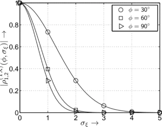
Fig. 2.Variation of the correlation coefficient|ρ(TX)1,2 (φ, σξ)|as a function ofσξ andφ
assuming an antennas separation in wavelengths ofdλ= 1/4
σ2
ξ. Calculating the expectation under this assumption leads to the following
equation:
ρ(TX)1,2 (φ, σξ) = ej 2π dλcos(φ)e
−1
2(2π dλsin(φ)σξ)2 . (6) When analysing Fig. 2 and Fig. 3, high valued correlation coefficients appear for small values ofφandσξ parameters. Additionally, in case of a small antenna
separation, i. e. reducingdλ, the received signalssr 1(t) andsr 2(t) become even
more similar.
2.2 Correlated MIMO System Model
The (nR×nT) system matrix H of a correlated MIMO system model is given by
vec(H) =R
1 2
HH·vec(G) , (7)
where Gis a (nR×nT) uncorrelated channel matrix with independent, iden-tically distributed complex-valued Rayleigh elements and vec(·) is the operator stacking the matrixGinto a vector column-wise [8]. Based on the quite common assumption that the correlation between the antenna elements at the transmit-ter side is independent from the correlation between the antenna elements at the receiver side, the correlation matrixRHH can be decomposed into a trans-mitter side correlation matrixRTX and a receiver side correlation matrix RRX following the Kronecker product ⊗. Under this assumption the matrixRHH is formulated as
RHH=RTX⊗RRX . (8)
In this paper, no correlation at the receiver side is assumed. Therefore, the (nR×nR) receiver-side correlation matrixRRX simplifies to
0 5 10 15 20 0 0.2 0.4 0.6 0.8 1 | ρ (T X ) 1 , 2 ( φ ,σ ξ ) | → σξ→
φ=30◦
φ=60◦
φ=90◦
Fig. 3.Variation of the correlation coefficient|ρ(TX)1,2 (φ, σξ)|as a function ofσξ andφ
assuming a wavelength specific antenna separation ofdλ= 1/16
with the matrix I describing the identity matrix. The (nR ×nR) correlation matrixRTX for the investigated (4×4) MIMO system is finally given by:
R(4TX×4)=
1 ρ(TX)1,2 ρ (TX) 1,3 ρ
(TX) 1,4 ρ(TX)2,1 1 ρ
(TX) 2,3 ρ
(TX) 2,4 ρ(TX)3,1 ρ
(TX)
3,2 1 ρ (TX) 3,4 ρ(TX)4,1 ρ
(TX) 4,2 ρ
(TX) 4,3 1
. (10)
Therein, the correlation coefficientρ(TX)k,ℓ describes the transmitter side correla-tion between the transmit antenna kandℓ. Taking line-of-sight conditions into account, the correlation coefficient results according to (4) in
ρ(TX)k,ℓ = e
−j 2π(k−ℓ)dλcos(φ) for k < ℓ . (11) Extending these results to scattered conditions, the transmitter side correlation coefficient results according to (5) fork < ℓin
ρ(TX)k,ℓ (φ, σξ) = e
−j 2π(k−ℓ)dλcos(φ)e−1
2(2π(k−ℓ)dλsin(φ)σξ)2 . (12) For the calculation of the transmitter-side correlation coefficient for values of k > ℓ it can be exploited that the values of the correlation coefficients are complex conjugated. This is due to the sign change when computing the distance difference between antennas with different antenna reference (see Fig. 4). Finally, the following equation can be used to calculate the correlation coefficient for values ofk > ℓ
ρ(TX)ℓ,k =ρ∗(TX)
k,ℓ . (13)
d1
d2
d/2 d/2 antenna #2
antenna #3
d antenna #1
antenna #1
d
antenna #4
d3
d4
Tx Rx
φ
Fig. 4.Antennas’ physical disposition: four transmit and one receive antennas
depicts the layer system model resulting after applying the singular value decom-position, where the weighting factors p
ξℓ,k represent the positive square roots
of the eigenvalues of the system matrix per MIMO layer ℓ and per transmit-ted data block k. The transmitted complex input symbol per MIMO layer ℓ is described bycℓ,kand the additive white Gaussian noise (AWGN) bywℓ,k,
respec-tively. In general, correlation influenced the unequal weighting of the different
cℓ,k yℓ,k
wℓ,k
p ξℓ,k
Fig. 5.Resulting system model per MIMO layerℓand transmitted data blockk
layers. In order to carefully study the influence of the correlation, two channel constellations are chosen as highlighted in Table 1. The corresponding unequal weighting of the different layers is shown in Fig. 6 and Fig. 7 for an exemplarily studied (4×4) MIMO system. Therein, the difference in the layer-specific fluc-tuations is described by the probability density function (pdf) of the parameter ϑ=p
ξℓ=4,k/pξℓ=1,k, which shows the unequal weighting of the different layers
within the MIMO system.
Table 1.Parameters of the of the investigated channel constellations
Description φ σξ dλ
Weak correlation 30◦ 1 1
Strong correlation 30◦ 1 0,25
0 0.1 0.2 0.3 0.4 0.5
0 0.005 0.01 0.015 0.02
uncorrelated correlated
p
d
f
→
ϑ →
Fig. 6.PDF (probability density function) of the ratioϑbetween the smallest and the largest singular value for weakly correlated (solid line) as well as uncorrelated (dotted line) frequency non-selective (4×4) MIMO channels (dλ= 1,φ= 30◦ andσξ= 1,0)
which is reached when all the layers have the same performance (assuming the same noise power at the receiver-side). In this particular case the layer-specific weighting factors, i. e., the singular values, are very similar. For weak antennas correlation, as depicted in Fig. 6, this parameter decreases which means some layers performs better than others and the overall MIMO channel performance drops. When antennas correlation is significantly high, the parameterϑbecomes smaller, meaning a noticeable difference in the performance of the various layer. Now, predominant strong and weak layers appear which decreases the overall channel performance (by increasing the BER).
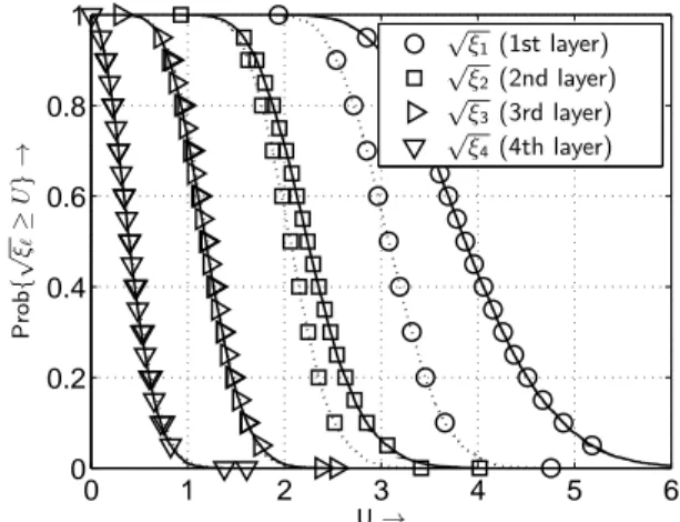
The distribution of the layer-specific characteristic can be studied when an-alyzing the CCDF (complementary cumulative distribution function) for the different degrees of correlation as shown in Fig. 8 and Fig. 9. The antennas cor-relation increases the probability of having layers with larger values (see layers
√
ξ1and√ξ2) and increases for weak layers the probability of having lower values (see layers√ξ3 and√ξ4).
0 0.1 0.2 0.3 0.4 0.5 0
0.005 0.01 0.015 0.02
uncorrelated correlated
p
d
f
→
ϑ →
Fig. 7.PDF (probability density function) of the ratioϑbetween the smallest and the largest singular value for strongly correlated (solid line) as well as uncorrelated (dotted line) frequency non-selective (4×4) MIMO channels (dλ= 1/4,φ= 30◦andσξ= 1,0)
performance is obtained. Weak correlation spreads the curves by right shifting those corresponding to the highest singular values increasing the probability of getting large values in contrast to the smallest singular values. Under strong antennas correlation the CCDF curve for the largest singular values are indeed more right shifted while the smallest ones are left shifted. In consequence, in this case the probability of the largest singular value to obtain a high value increases while the probability of taking the smallest singular values a lower value also increases dealing to the MIMO channel worse performance.
3
Bit- and Power Assignment
AssumingM-ary Quadrature Amplitude Modulation (QAM), the argument̺= U2
A/UR2 of the complementary error function [4, 9] can be used to optimize the quality of a data communication system by taking the half-vertical eye-opening UAand the noise power per quadrature componentUR2 at the detector input into account [1]. The half-vertical eye-opening per MIMO layerℓand per transmitted symbol blockkresults in
UA(ℓ,k)=
p
ξℓ,k·Usℓ , (14)
where Usℓ denotes the half-level transmit amplitude assuming Mℓ-ary QAM
and p
ξℓ,k represents the positive square roots of the eigenvalues of the matrix
HHH. The average transmit powerPsℓ per MIMO layerℓdetermines the
half-level transmit amplitude Usℓ and is given by
Psℓ=
2 3U
2
0 1 2 3 4 5 6 0
0.2 0.4 0.6 0.8
1 √
ξ1(1st layer)
√
ξ2(2nd layer)
√
ξ3(3rd layer)
√
ξ4(4th layer)
P
ro
b
{
√ ξ
ℓ
≥
U
}
→
U→
Fig. 8.CCDF of the layer-specific distribution for weakly correlated (solid line) as well as uncorrelated (dotted line) frequency non-selective (4×4) MIMO channels (dλ= 1,
φ= 30◦ andσ
ξ= 1,0)
Activating L ≤ min(nT, nR) MIMO layers, the overall transmit power Ps =
PL
ℓ=1Psℓcan be calculated.
Power Allocation (PA) can be used to balance the BER in the different numbers of activated MIMO layers [1]. The resulting layer-specific system model including power allocation is highlighted in Fig. 10. The layer-specific power allocation factors√pℓ,k adjust the half-vertical eye opening according to
UA PA(ℓ,k)=√pℓ,k·
p
ξℓ,k·Usℓ . (16)
This results in the layer-specific transmit power per symbol blockk
Ps PA(ℓ,k)=pℓ,kPsℓ . (17)
Taking all activated MIMO layers into account, the overall transmit power per symbol blockkis obtained as
Ps PA(k) =
L
X
ℓ=1
Ps PA(ℓ,k)=Ps . (18)
In order to balance the BER in the different numbers of activated MIMO layers, solutions for the so far unknown PA parameters are needed.
0 1 2 3 4 5 6 0
0.2 0.4 0.6 0.8
1 √
ξ1(1st layer)
√
ξ2(2nd layer)
√
ξ3(3rd layer)
√
ξ4(4th layer)
P
ro
b
{
√ ξ
ℓ
≥
U
}
→
U→
Fig. 9.CCDF of the layer-specific distribution for strongly correlated (solid line) as well as uncorrelated (dotted line) frequency non-selective (4×4) MIMO channels (dλ= 1/4,
φ= 30◦ andσ
ξ= 1,0)
cℓ,k yℓ,k
wℓ,k
p ξℓ,k
√p ℓ,k
Fig. 10.Resulting layer-specific system model including MIMO-layer PA
for the signal-to-noise ratio at the detector input
̺(PAℓ,k)=
UA PA(ℓ,k)2 U2
R
= constant ℓ= 1,2, . . . , L . (19)
When assuming an identical detector input noise varianceU2
R for each channel output symbol the beforehand introduces Equal-SNR criteria requires the same half vertical eye opening of each channel output symbol
UA PA(ℓ,k)= constant ℓ= 1,2, . . . , L . (20) The power to be allocated to each activated MIMO layerℓand transmitted data blockkcan be shown to be calculated as follows:
pℓ,k=
1 U2
sℓ·ξℓ,k
· L L
P
ν=1 1
U2 sν·ξν,k
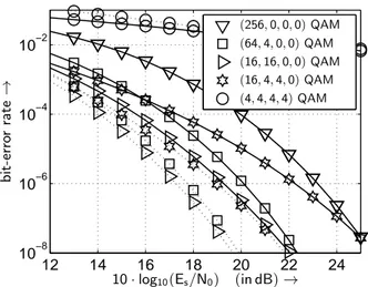
Table 2.Investigated QAM transmission modes throughput layer 1 layer 2 layer 3 layer 4
8 bit/s/Hz 256 0 0 0
8 bit/s/Hz 64 4 0 0
8 bit/s/Hz 16 16 0 0
8 bit/s/Hz 16 4 4 0
8 bit/s/Hz 4 4 4 4
and guarantees for each channel output symbol (ℓ = 1, . . . , L) the same half vertical eye opening of
UA PA(ℓ,k)=√pℓ,k·
p
ξℓ,k·Usℓ=
v u u u t
L
L
P
ν=1 1
U2 sνξν,k
. (22)
Together with the identical detector input noise variance for each channel output symbol, the above-mentioned equal quality scenario is encountered.
4
Results
In this work a (4×4) MIMO system with transmitter-side antennas correlation is studied.
In order to transmit at a fixed data rate while maintaining the best possible integrity, i. e., bit-error rate, an appropriate number of MIMO layers has to be used, which depends on the specific transmission mode, as detailed in Table 1.
The choice of fixed transmission modes regardless of the channel quality can be justified when analyzing the probability of choosing a specific transmission mode by using optimal bit loading [12]. As highlighted in Table 3 for uncorrelated MIMO channels, it turns out that only an appropriate number of MIMO layers has to be activated, e. g., the (16,4,4,0) QAM configuration. However, when
Table 3. Probability of choosing specific transmission modes at a fixed data rate by using optimal bitloading (10·log10(Es/N0) = 10 dB)
mode (64,4,0,0) (16,16,0,0) (16,4,4,0) (4,4,4,4) pdf 0.0116 0.2504 0.7373 0.0008
Table 4. Probability of choosing specific transmission modes in weakly correlated MIMO channels at a fixed data rate by using optimal bitloading (10·log10(Es/N0) = 10
dB)
mode (64,4,0,0) (16,16,0,0) (16,4,4,0) (4,4,4,4) pdf 0.1274 0.3360 0.5366 0.0
Table 5. Probability of choosing specific transmission modes in strongly correlated MIMO channels at a fixed data rate by using optimal bitloading (10·log10(Es/N0) = 10
dB)
mode (64,4,0,0) (16,16,0,0) (16,4,4,0) (4,4,4,4) pdf 0.8252 0.1087 0.0605 0.0
well as in Table 5 for highly correlated MIMO channels, the importance of using layers with large singular values increases.
The optimal performance results when using PA are shown in Fig. 11 and Fig. 12: The BER becomes minimal in case of an optimized bit loading with highest bit loading in the layer with largest singular values.
Fig. 13 and 14 show the MIMO system performance when using fixed trans-mission modes and having different degrees of correlation. As highlighted by the BER curves, in case of high correlation only the layers with the largest singular values should be used for the data transmission.
5
Conclusion
12 14 16 18 20 22 24
10−8
10−6
10−4
10−2
10·log10(Es/N0) (in dB)→
b
it
-e
rr
or
ra
te
→
(256,0,0,0)QAM (64,4,0,0)QAM (16,16,0,0)QAM (16,4,4,0)QAM (4,4,4,4)QAM
Fig. 11.BER with optimal PA (dotted line) and without PA (solid line) when using the transmission modes introduced in Tab. 2 and transmitting 8 bit/s/Hz over frequency non-selective (4×4) MIMO channels (dλ = 1, φ = 30◦ and σξ = 1,0) with weak
transmitter-side correlation
12 14 16 18 20 22 24
10−8
10−6
10−4
10−2
10·log10(Es/N0) (in dB)→
b
it
-e
rr
or
ra
te
→
(256,0,0,0)QAM (64,4,0,0)QAM (16,16,0,0)QAM (16,4,4,0)QAM (4,4,4,4)QAM
Fig. 12.BER with optimal PA (dotted line) and without PA (solid line) when using the transmission modes introduced in Tab. 2 and transmitting 8 bit/s/Hz over frequency non-selective (4×4) MIMO channels (dλ = 1/4, φ= 30◦ and σξ = 1,0) with strong
12 14 16 18 20 22 24
10−8
10−6
10−4
10−2
10·log10(Es/N0) (in dB)→
b
it
-e
rr
or
ra
te
→
no Correlation weak Correlation strong Correlation
Fig. 13.BER with optimal PA (dotted line) and without PA (solid line) when using the (16,16,0,0 QAM transmission mode and transmitting 8 bit/s/Hz over frequency non-selective (4×4) MIMO channels with different degrees of correlation
12 14 16 18 20 22 24
10−8
10−6
10−4
10−2
10·log10(Es/N0) (in dB)→
b
it
-e
rr
or
ra
te
→
no Correlation weak Correlation strong Correlation
The analysis has demonstrated that the representation of the PDF of the ratio between the smallest and the largest singular values provides a useful mean to predict the channel behavior and the appropriateness of activating all the MIMO layers. Besides, the singular values CCDF gives relevant information concerning the probability of obtaining predominant (strong and weak) layers and infer the MIMO channel behaviour. The best performance is obtained when all CCDF coincide (are the same) or are quite close. CCDF curve dispersion reveals the existence of predominant layer lowering the MIMO performance. Additionally, in order to mitigate correlation effects the investigation has analyzed the effect of bit and transmit power allocation along the various MIMO layers as techniques for improving channel performance even in the presence of antennas correlation. Regarding the power allocation, a basic technique has been applied in order to obtain the same quality along the different activated layers, i.e., the same SNR at each detector. This technique allows obtaining a higher performance. Moreover, bit loading has been studied through the description of some profiles (transmission modes) dealing to different constellation per layer (bit per symbol interval) but maintaining the overall transmission rate. A remarkable conclusion is that activating all the MIMO layers not necessarily provides the best perfor-mance as highlighted in the results where the transmission modes (64,4,0,0) and (16,16,0,0) present the best performance. In order to highlight the importance of this fact the probability of using each transmission mode was analyzed and the previous conclusion was remarked.
References
1. Ahrens, A. and Lange, C. (2008). Modulation-Mode and Power Assignment in SVD-equalized MIMO Systems. Facta Universitatis (Series Electronics and Ener-getics), 21(2):167–181.
2. Cano-Broncano, F., Benavente-Peces, C., Ahrens, A., Ortega-Gonzalez, F. J., and Pardo-Martin, J. M. (2013). Analysis of MIMO Systems with Transmitter-Side Antennas Correlation. In International Conference on Pervasive and Embedded Computing and Communication Systems (PECCS), Barcelona (Spain).
3. Haykin, S. S. (2002). Adaptive Filter Theory. Prentice Hall, New Jersey.
4. Kalet, I. (1987). Optimization of Linearly Equalized QAM.IEEE Transactions on Communications, 35(11):1234–1236.
5. K¨uhn, V. (2006). Wireless Communications over MIMO Channels – Applications to CDMA and Multiple Antenna Systems. Wiley, Chichester.
6. Lee, W.-Y. (1973). Effects on Correlation between two Mobile Radio Base-Station Antennas. IEEE Transactions on Vehicular Technology, 22(4):130–140.
7. Mutti, C. and Dahlhaus, P. (2004). Adaptive Power Loading for Multiple-Input Multiple-Output OFDM Systems with Perfect Channel State Information. InJoint COST 273/284 Workshop on Antennas and Related System Aspects in Wireless Communications, pages 93–98, Gothenburg.
10. Salz, J. and Winters, J. H. (1994). Effect of Fading Correlation on adaptive Arrays in digital Mobile Radio. IEEE Transactions on Vehicular Technology, 43(4):1049– 1057.
11. Shiu, D., Foschini, G., Gans, M., and Kahn, J. (2000). Fading Correlation and its Effect on the Capacity of Multielement Antenna Systems. IEEE Transactions on Communications, 48(3):502–513.
12. Wong, C. Y., Cheng, R. S., Letaief, K. B., and Murch, R. D. (1999). Multiuser OFDM with Adaptive Subcarrier, Bit, and Power Allocation. IEEE Journal on Selected Areas in Communications, 17(10):1747–1758.