K-means algorithms for functional data

K

-means algorithms for functional data

María Luz López García

a

, Ricardo García-Ródenas

a,n

, Antonia González Gómez

b a

Departamento de Matemáticas, Escuela Superior de Informática, Universidad de Castilla la Mancha, 28012 Ciudad Real, Spain b

Departamento de Matemática Aplicada a los Recursos Naturales, E.T. Superior de Ingenieros de Montes, Universidad Politécnica de Madrid, 28040 Madrid, Spain

a r t i c l e i n f o

Keywords:

Functional data

K-means

Reproducing Kernel Hilbert Space Tikhonov regularization theory Dimensionality reduction

a b s t r a c t

Cluster analysis of functional data considers that the objects on which you want to perform a taxonomy are functionsf:XRp_{↦Rand the available information about each object is a sample in afinite set of} pointsf_n¼ fðxi;yiÞAXRgni¼1. The aim is to infer the meaningful groups by working explicitly with its infinite-dimensional nature.

In this paper the use ofK-means algorithms to solve this problem is analysed. A comparative study of threeK-means algorithms has been conducted. TheK-means algorithm for raw data, a kernelK-means algorithm for raw data and aK-means algorithm using two distances for functional data are tested. These distances, calleddVn anddϕ, are based on projections onto Reproducing Kernel Hilbert Spaces (RKHS)

and Tikhonov regularization theory. Although it is shown that both distances are equivalent, they lead to two different strategies to reduce the dimensionality of the data. In the case ofdVn distance the most

suitable strategy is Johnson–Lindenstrauss random projections. The dimensionality reduction ford_ϕis based on spectral methods.

A key aspect that has been analysed is the effect of the samplingfxign

i¼1on theK-means algorithm performance. In the numerical study anex professoexample is given to show that if the sampling is not uniform inX, then aK-means algorithm that ignores the functional nature of the data can reduce its performance. It is numerically shown that the originalK-means algorithm and that suggested here lead to similar performance in the examples whenXis uniformly sampled, but the computational cost when working with the original set of observations is higher than theK-means algorithms based ond_ϕordVn,

as they use strategies to reduce the dimensionality of the data.

ThenumericaltestsarecompletedwithacasestudytoanalysewhatkindofproblemtheK-means algorithmforfunctionaldatamustface.

1. Introduction

Cluster analysis allows data structures to be explored. These tools provide afirst intuitive data structure by identifying mean-ingful groups. Two essential elements in cluster analysis are data

representation and the specification of similarity between them.

Most of these methods assume that the objects can be represented

as points in Euclidean spacesRn_{;but for some problems data are}

random functions (physical processes, genetic data, chemical spec-tra, voice recording, control processes, etc). In this paper we assume

that the objects are functions f:XRp_{↦R and the information}

provided by each of them is a sampling of a finite set of points

fn¼ fðxi;yiÞAXRgni¼1. The aim is to infer the data structure by

working explicitly with their infinite dimensional nature in Hilbert spaces. Thisfield is known asfunctional data analysis(FDA)[29,11]. Jacques and Preda [17]establish a classification of the different clustering methods for functional data as follows: (i) raw-data clustering, (ii) two-stage methods, (iii) non-parametric clustering and (iv) model-based clustering. A similar classification for clustering

of time-series data is proposed by Liao [22]. The methods of type

(i) work directly with raw data, type (ii) indirectly with features extracted from the raw data, type (iii) use a specific distance or dissimilarity between functions and type (iv) with models built from the raw data, in which the estimation of features and clustering are performed simultaneously.

Methods (ii)–(iv) developed in functional data clustering use

Hilbert spaces to tackle the functional nature of the data and to obtain a representation of these data. Many of the methods choose an orthogonal basis of functions

Φ

¼ f

φ

1;…;

φ

Lg with LAN and each functional datum is represented as a linear combination of the vectors in the basis

Φ

. Usual choices of

Φ

are Fourier,Waveletsor

B-splines. In this paper following[15], we consider each function as n_{Corresponding author.}

E-mail addresses:MariaLuz.Lopez@uclm.es(M. Luz López García), ricardo.garcia@uclm.es(R. García-Ródenas),

a point in a general function space and then project these points onto a Reproducing Kernel Hilbert Space (RKHS) by using the Tikhonov regularization theory. This mechanism induces a distance among the functions of the sample and therefore it allows cluster-ing algorithms to be applied to functional data. This process is completed with a strategy for dimensionality reduction consisting

of a new projection onto a finite-dimensional Euclidean space

which makes the distance between the functions coincide with the Euclidean distance of the projected data. The method proposed in this paper is an instance of a two-stage method but it allows the algorithms of this class to be reinterpreted (mainly based on it functional principal component analysis) as methods that compute the similarity measure as the distance between the projections of the data onto a Hilbert space.

The mathematical theory of RKHS[25]has been applied to several fields such assupport vector machines(SVM)[9],principal component analysis[30],canonical correlation analysis[13]andFisher's discrimi-nant analysis[26]. RKHS has also been applied tofinite-dimensional cluster analysis giving rise to the so-called kernel-based clustering methods. Filippone et al.[12]classify clustering methods based on kernels into three categories: (i) methods based on kernelization of the distance, (ii) clustering infeature spacesand (iii) methods based on SVM. It has been experimentally shown that methods based on kernels allow correct grouping of clusters with nonlinear borders.

This paper is focused on theK-means algorithm [24], which

may have been the most popular clustering algorithm since the

60s. This algorithm has been deeply range-studied in the finite

case[33]and it has been extended to many situations asK-means

based on kernels, see[30,14,8].

Cadre and Paris[5]developed a numericalK-means algorithm

for infinite-dimensional Hilbert spaces. This numerical scheme

discretizes functions on grids and considers that all grid cells have the same volume. These authors show that the theoretical perfor-mance of this algorithm matches the classical.

Functional data clustering has also been addressed by theK-means

algorithm in [1,28]. As a _first step the dimension of the data is

reduced, and then as a second step theK-means forfinite dimensional data is used. In[1]the dimension reduction strategy consists of an

approximation of the curves into a _finite B-spline basis and the

B-spline coefficients are used as feature vectors. Peng and Müller[28]

use principal component scores to reduce the dimensionality. Yao

et al.[37]introduce the kernel approximately harmonic projection

(KAHP) which is a suitable strategy to reduce dimensionality of

the data in combination with the K-means algorithm in a fi

nite-dimensional context. Chen and Li[7]propose the use of a Johnson–

Lindenstrauss type random projection as a preprocessing for func-tional learning algorithms. These ideas are adapted to this work in a context of functional data clustering, as Biau et al. [3]. A second strategy based on spectral methods is introduced.

We discuss numerical aspects ofK-means algorithms for cluster

analysis in infinite-dimensional Hilbert spaces. The proposed

algo-rithm, named KK-means, consists of applying theK-means algorithm

to functional data using projections on RKHS. The contributions of this paper can be summarized as follows:

An interpretation of the two-stage methods based on principal

component analysis is given. These approaches calculate the distance between the empirical functions as the distance between their projections onto function spaces. In this paper two types of projections have been proposed (in two different bases) using the Tikhonov regularization theory.

A numerical study is conducted using (i) theK-means algorithm

applied to a raw data, (ii) the approximate kernelK-means (aKKm,

[8]) and (iii) the KK-means algorithm. By means of the Kappa

coefficient of agreement, it is shown that if the data are sampled at regular time intervals the functional nature of the data can be

ignored without damaging the performance of the clust-ering procedure. This is a numerical validation of the theoretical

result of[5]. A numerical counter-example has been included,

with a non-uniform discretization strategy, for raw-data cluster-ing methods in which the performance of aKKm and the

K-means algorithm is significantly deteriorated compared with

the KK-means algorithm, which accounts for the functional nature.

The effectiveness of a dimension reduction strategy based on the

number of eigenfunctions has been numerically demonstrated. It was found that when data are uniformly sampled, KK-means

and aKKm have a significantly lower computational cost than a

K-means algorithm applied to raw data.

In Section 2 we develop metrics for empirical functions and establish relationships to calculate them by the Euclidean distance

between projections infinite dimensional spaces. In Section 3we

carry out a numerical experiment to evaluate the performance of the proposed algorithms and analyse a case study. Finally, inSection 4

we gather together the conclusions obtained.

2. Projecting functional data onto reproducing Kernel Hilbert spaces

Fig. 1shows the contents of this section schematically. As afirst step, we project the empirical functions onto a Reproducing Kernel

Hilbert Spaces (RKHS)HK applying the Tikhonov regularization

theory in RKHS. Following González-Hernández[15]we use two

representations of these projections, one using kernel expansions

and the other eigenfunctions. We define the distance between two

empirical functions as the distance inHK between their

projec-tions. Secondly, we use Cholesky decomposition to show that this distance between functions can be calculated by the Euclidean distance between a data transformation. This theoretical result presents two meaningful advantages: (i) it allows the use of the

vectorialK-means algorithm codes for functional data and (ii) as

the Johnson–Lindenstrauss-type random projections to reduce the

dimensionality requires working with Euclidean distance, this transformation enables it to be used. Other theoretical

contribu-tions are set out inAppendix Awhich it shows that the proposed

scheme (depicted in Fig. 1) coincides with functional principal

component analysis (FPCA) in which projections are performed

using the Tikhonov regularization theory. This identification

allows us to interpret the FPCA as a cluster method in which the similarity measure is the distance between projected functions.

This section begins with a brief revision of RKHS and the Tikhonov regularization theory in RKHS. The general theory of

Empirical functions (Raw data)

{(xi,yi)}

Projections of functional data

Reproducing Kernel Hilbert

Space (RKHS)

s-Dimensional Euclidean Space

(Euclidean distance)

Metric transformation

Tikhonov regularization is in the book of [34] and the general theory of RKHS is in[2].

Definition 1 (Reproducing Kernel). LetHbe a real Hilbert space of

functions de_fined inXRp_{with inner product}

;

h iH. A function

K:XX↦Ris called a Reproducing Kernel ofHif

1. Kð;xÞAHfor allxAX.

2. fðxÞ ¼f;Kð:xÞ_H for allfAHand for allxAX.

We define the norm by‖f‖H¼f;f1_H=2

A Hilbert space of functions that admits a Reproducing Kernel is

called aReproducing Kernel Hilbert Space(RKHS). The reproducing

Kernel of a RKHS is uniquely determined. Conversely, if K is a

positive definite and symmetric kernel (Mercer kernel), then it

generates a unique RKHS in which the given kernel acts like a Reproducing Kernel.

For our purpose we list the fundamental properties of RKHS:

Theorem 1. Let H be a real Hilbert space of functions defined in XRp_{with inner producth i;}

H. Let K:XX↦Rbe a Reproducing

Kernel ofH. Then it follows that

(a) Kðx;yÞ ¼Kð;xÞ;Kð;yÞ_Hfor all x;yAX. (b) ‖f‖2

H¼∑ni¼1∑nj¼1

α

i

α

jKðxi;xjÞfor all fAHwhere

f¼ ∑n i¼1

α

iKð;xiÞ

with xiAX.

(c) Let LKðfÞðxÞ ¼RXKðx;yÞfðyÞdy with fAL

2_{ðXÞ. Mercer's Theorem}

asserts that

Kðx;yÞ ¼ ∑1 j¼1

λ

j

ϕ

jðxÞ

ϕ

jðyÞ;

where

ϕ

j is the j-th eigenfunction of LKand

λ

jits corresponding

non-negative eigenvalue. (d) The function spaceHis given by

H¼ f_AL2_ðXÞ

: ∑1 j¼1

λ

1

j f;

ϕ

j

D E

L2_ðXÞ

2

o1

( )

ð1Þ

and the inner product can be written as

f;g

H¼ ∑ 1

j¼1

λ

1

j f;

ϕ

j

D E

L2_ðXÞ g;

ϕ

j

D E

L2_ðXÞwith f;gAH: ð2Þ

Now we brie_fly describe the Tikhonov discrete regularization

for the problem at hand. Let K be a Mercer kernel and HK its

associated RKHS. Consider a subset compactXRp_{and let}

ν

_{be a}

Borel probability measure inXR. Let the regression function

f_νðxÞ ¼ Z

Rdνðy xÞ

ð3Þ

whered_νðyjxÞis the conditional probability measured onR. Both

ν

andf_νare unknown and what we want is to reconstruct this mean

function. Let

Xn≔fx1;…;xng X

and letfnbe a random sample independently drawn from

ν

andf_ν

onX. That is

fn≔fðxi;yiÞAXRg n i¼1:

The Tikhonov regularization considers the function space

Vn≔spanKð;xÞ:xAXn ð4Þ

wherespanis the linear hull and projectsf_ν onto this space by

using the samplefn. The Tikhonov regularization theory makes a

stable reconstruction off_νby solving the following optimization

problem:

fn≔arg min fAVn

1

n ∑

n

i¼1

fðxiÞyi 2

þ

_γ

‖f‖2

HK ð5Þ

where

γ

40 and‖f‖HKrepresents the norm offinHK. The solution

fn of (5) is called the Regularized

γ

-Projection of f_ν onto HK associated to the samplefn.

The Regularized

γ

-Projection offnn belongs toVnHK and for this reason it can be expressed as a linear combination of any basis ofHK. In the next subsection we calculate these projections onto

two basis of HK. The first basis consists of the functions

fKðx;xiÞ: xiAXng and the second one consists of eigenfunctions f

_ϕ

1;

ϕ

2;⋯gof the integral operatorLK.

2.1. Kernel representation and associated distance

Therepresentationtheorem gives a closed form solution offn

for the optimization problem (5). This theorem was introduced

by Kimeldorf and Wahba[19] in a spline smoothing context and

has been extended and generalized to the problem of minimizing risk of functions in RKHS, see[31,10].

Theorem 2 (Representation). Let fn be a sample of f_ν, let K be a

(Mercer) kernel and let

γ

40. Then there is a unique solution fnof(5)

that admits a representation by

fnðxÞ ¼ ∑n i¼1

α

iKðx;xiÞ; forall xAX; ð6Þ

where

α

¼ ð

_α

1;…;

α

nÞT is a solution to the linear equation systems:

ð

_γ

nInþKxÞ

α

¼y; ð7Þ

whereInis the identity matrix nn,y¼ ðy1;…;ynÞT and the matrix

Kx is given by Kð xÞij¼Kðxi;xjÞ. The expression (6) leads to the

estimate of f_νin Xn b

f n¼Kx

α

ð8Þ

Theorem 1(b) establishes that the norm offinVnis given by the following inner product:

‖f‖2

Vn¼

α

T

Kx

α

; for allfAVn: ð9Þ

As Kx is a symmetric positive definite matrix it admits the

decomposition

Kx¼VTDV ð10Þ

where the rows of the matrixVare the eigenvectors of the matrix

Kx and Dis a diagonal matrix whose diagonal entries are the

corresponding (non-negative) eigenvalues. Therefore,

Kx¼ ðD1=2VÞTðD1=2VÞ ¼UTU ð11Þ withU¼D1=2V. Using the Cholesky decomposition(11)

‖f‖2

Vn¼

α

T_K

x

α

¼

α

TUTU

α

¼

α

~T

α

~¼‖

α

~‖2 ð12Þ

with

α

~¼U

α

. This expression shows that the norm of fðxÞ ¼

∑n

i¼1

α

iKðx;xiÞ, with xiAXn, in Vn coincides with the Euclidean norm of a transformation of the space, that is‖

α

~‖.

Definition 2 (Distance dVn). LetXbe a compact set and

ν

,

μ

two Borel

probability measures defined onXR. LetK:XX↦Rbe a Mercer kernel andHKits associated RKHS. Letf_νandg_μbe functions defined as (3). Let fn≔fðxi;yiÞAXRg

n

i¼1 and gn≔fðxi;y0iÞAXRg n i¼1 be

two samples of the previous functions obtained from the probability distributions

ν

and

μ

. Suppose that the Regularized

γ

-Projection of these functions arefnðxÞ ¼∑n

We define the square of the distancedVnfromfntognby

d2Vnðfn;gnÞ≔‖f

n_gn_‖2

Vn¼ ð

α

β

Þ

T_K xð

α

β

Þ

¼ ð

_α

_β

ÞT_UT_Uð

_α

_β

_{Þ ¼‖Uð}

_α

_β

_Þ‖2

¼‖U

α

U

β

‖2_¼‖

_α

_~

_β

~_‖2 _ð13Þ

where

α

~≔U

α

and

β

~≔U

β

.

2.2. RKHS representation and associated distance

González-Hernández[15]introduces an alternative

representa-tion for sampling funcrepresenta-tions in RKHS.

Theorem 3 (RKHS representation). Let X be a compact set and let

ν

be a Borel probability measure defined on XR. Let K:XX↦Rbe a Mercer kernel andHK its associated RKHS. Let f_νbe defined by(3)

and fn¼ fðxi;yiÞAXRga sample of fνdrawn from the probability

distribution

ν

. Let LK be the integral operator associated with the

kernel K and letf

λ

1;

λ

2;…gbe the eigenvalues of LKandf

ϕ

1;

ϕ

2;…g

the corresponding eigenfunctions. Then the projection fngiven by the minimization of(5)can be written by

fnðxÞ ¼∑ j

α

ϕ

j

ϕ

jðxÞ ð14Þ

where

α

ϕ_j are the weights of the projection of fnonto the function space RKHS generated by the eigenfunctions

ϕ

1ðxÞ;

ϕ

2ðxÞ;…

. In practice, when a finite sample is available, the first srrankðKxÞ

weights

α

ϕ_j can be estimated by

b

α

ϕj ¼

ℓj ffiffiffi

n

p ð

_α

T_v

jÞ; j¼1;…;s; ð15Þ

where ℓj is the j-th eigenvalue of the matrix Kx, vj is the j-th

eigenvector of Kx and

α

is the solution to Eq.(7).This leads to the

approximation:

fnðxÞ ¼∑ j

α

ϕ

j

ϕ

jðxÞffi ∑ s

j¼1

b

α

ϕ

j

ϕ

jðxÞ: ð16Þ

The functions

ϕ

jðxÞare unknown but they can be approximated at

the sampling points xi by

ϕ

bjðxiÞ ¼ ffiffiffin p

vji to obtain the following

approximation: b

f nffipffiffiffin ∑s j¼1

b

α

ϕ

jvj; ð17Þ

wherebfn¼ ðbfnðx1Þ;…;bf n

ðxnÞÞT.

Definition 3 (Empirical

γ

-regularized distance d_ϕ). Let X be a

compact set and let

ν

and

μ

be two Borel probability measures

defined onXR. LetK:XX↦Rbe a Mercer kernel andHK its

associated RKHS. Let f_ν and g_μ be functions defined as (3). Let

fn≔fðxi;yiÞAXRgni¼1andgn≔fðxi;y0iÞAXRg n

i¼1be two samples

of the previous functions drawn from the probability distributions

ν

and

μ

. Suppose that the Regularized

γ

-Projection of these

functions isfnðxÞffi∑s

j¼1

α

bϕj

ϕ

jðxÞandgnðxÞffi∑sj¼1

β

b

ϕ j

ϕ

jðxÞ.

We de_fine the square of the empirical distance d_ϕ from fn

tognby

d2_ϕðfn;gnÞ≔‖fngn‖2HK¼ f

n_gn_;fn_gn

HK ð18Þ

¼ ∑1 j¼1

λ

1

j fngn;

ϕ

j

D E

L2_ðXÞ

ϕ

j;f n_gn

D E

L2_ðXÞ ð19Þ

¼ ∑s j¼1

ð

α

bϕj

β

b ϕ j Þ2

λ

j :

ð20Þ

Following González-Hernández[15]and Smale and Zhou[32]the

eigenvalues and eigenvectors ofKx=nconverge to the eigenvalues

and eigenfunctions ofLK, and we have

λ

jffiℓj

n ð21Þ

and we obtain the following approximation:

d_ϕðfn;gnÞffi

ffiffiffiffiffiffiffiffiffiffiffiffiffiffiffiffiffiffiffiffiffiffiffiffiffiffiffiffiffiffiffiffiffiffi

∑s j¼1

nð

α

bϕj

β

b ϕ j Þ 2 ℓj v u u u

t ¼‖

α

~ϕ

_β

~ϕ_{‖ ð22Þ}

where ‖‖ is the Euclidean norm,

α

~ϕ≔pffiffiffinDs1=2

α

bϕ,

β

~ ϕ

≔ ffiffiffi

n

p

Ds1=2

β

b ϕ

andDs1=2is the matrixss

Ds1=2¼

1_ffiffiffiffi

ℓ1

p _{0 ⋯ 0}

0 1_ffiffiffiffi

ℓ2 p _{⋯ 0}

0 0 ⋯ 1_ffiffiffiffi

ℓs p 0 B B B @ 1 C C C A:

2.3. Dimensionality reduction strategies for each distance dVnand dϕ

The functional data, due to their nature, in most cases are of very high dimension. This leads the application of the cluster algorithms to require high CPU times and intensive use of the RAM. In this subsection we discuss (i) how to reduce the original data representation according to the distanced_ϕordVnand (ii) the

relationship between the two distances.

First we discuss the question (ii). Let us see that the distances

dVnanddϕcoincide fors¼n. The distancesdVnanddϕproject the

original data and thus the Euclidean distance for projected data is calculated. Let us check that fors¼nboth projections coincide. Let

~

α

ϕ_and

_α

_{~ be the projection of the functionf}

nonto RKHS and the

kernel respectively. In this case D¼Dn and the coefficients

α

bϕ, given by(15), are written in the matrix form:

b

α

ϕ¼ 1ffiffiffi

n

p DV

α

ð23Þ

therefore ifs¼n

~

α

ϕ_¼pffiffiffi_nD1=2

s

α

bϕ¼D 1=2

DV

α

¼U

α

¼

α

~: ð24Þ This is the expected result since the distances are based on two representations in different basis of the same function. The essential difference between these two approaches is how they reduce the dimension of the data.

2.3.1. Dimensionality reduction by working with d_ϕ

According to the relationships set out inAppendix Awith FPCA,

it follows that a dimension reduction strategy must be based on the magnitude of the eigenvalues fℓjg. Let fℓ1;…;ℓsg be the s

largest eigenvalues ofKxandVsthe matrix whose rows are thes

eigenvectors. In this case the matrix of projection is

Ps¼D1s=2Vs: ð25Þ

2.3.2. Johnson–Lindenstrauss-type random projections to reduce dimensionality by working with dVn

We now analyze Johnson–Lindenstrauss-type random

projec-tions to reduce the dimensionalitynof the data as described in[3]. The key idea that enables the use of these projections is that the distances between the empirical functions are calculated by the Euclidean distance of the transformed data.

Given s a positive integer and s sequences of independent

random variables ðM1;iÞiZ1⋯ðMs;iÞiZ1 with normal distribution

with mean 0 and variance 1/s, we de_fine

Ms≔

M11 ⋯ M1n

⋮ ⋮ ⋮

A random projection using the linear function M:Rn_↦Rs _with

Mð

_α

Þ ¼Ms

α

is defined. The next lemma[3]states how to choose the value ofs.

Lemma 1 (Johnson–Lindenstrauss Lemma). For any

ε

;

δA

ð0;1Þand any positive integer N, let s be a positive integer such that

s_Z4ð

ε

2 =2

ε

3

=3Þ1_log N_ffiffiffi

δ

p _:

Then, for any set D of N points and for all ð

α

~;

β

~ÞADD with probability1

_δ

,the following holds:

ð1

_ε

Þ‖

α

~

_β

~‖r‖Ms

α

~Ms

β

~‖rð1þ

ε

Þ‖

α

~

β

~‖: ð26Þ

The Johnson–Lindenstrauss lemma guarantees that the

dis-tance derived from the standard Euclidean product is preserved in the set ofNoriginal data points. Applying this to our case:

dVnðfn;gnÞ ¼‖

α

~

β

~‖ffi‖MsU

α

MsU

β

‖ ð27Þ where

α

~≔U

α

and

β

~≔U

β

. The matrix of projection, for the metric

dVn, is

Ps¼MsU: ð28Þ

2.4. The K-means algorithm for functional data

In this section we synthesize the above results into aK-means

algorithm for functional data. In essence, the functional data are

projected onto asdimensional space and theK-means algorithm

infinite-dimensional spaces is applied to the functional data. The

K-means algorithm for functional data is described inTable 1.

Remark 1. This paper addresses the critical issue of cluster analysis in calculating distance between empirical functions so these results are efficiently applicable to many clustering schemes. Observe that once the functional data are projected in Step 1, any other clustering algorithm, such as hierarchical clustering, could have been applied in Step 2.

3. Numerical trials

In this section several numerical experiments are performed. Our main goals are:

To determine when it is necessary to consider explicitly the

functional nature of the data that we wish to analyse. To do

this, we will compare numerically the basicK-means algorithm

and a kernelK-means algorithm, specifically the approximate

kernelK-means (aKKm) applied to raw data with the KK-means

algorithm.

To determine the advantages of considering distances derived

from the functional projections.

To analyze the effect of the dimensionality reduction parameter

sused tod_ϕin the performance of KK-means algorithm.

To provide the methodology described with a real example and

to identify what difficulties must be addressed.

The first three questions are addressed in Experiments1a–1c

and the third goal inExperiment2.

3.1. Description of the numerical experiments

3.1.1. Test problems

The test problems used in the numerical experiments are:

Waves: These data are obtained by a convex combination of triangular waves[4]defined as follows (seeFig. 2):

y1ðxÞ ¼uh1ðxÞþð1uÞh2ðxÞþ

ε

ðxÞfor the class 1;

y2ðxÞ ¼uh1ðxÞþð1uÞh3ðxÞþ

ε

ðxÞfor the class 2;

y3ðxÞ ¼uh2ðxÞþð1uÞh3ðxÞþ

ε

ðxÞfor the class 3;

where u is a uniform random variable in ð0;1Þ;

ε

ðxÞ is a standard normal variable and the functionshkare the following triangular waves inxA½1;21:

h1ðxÞ≔maxð6jx11j;0Þ; h2ðxÞ ¼h1ðx4Þ; h3ðxÞ ¼h1ðxþ4Þ

The data generated are shown inFig. 3.

Signals with different type of noise: This test problem is

described in [21]. It starts with a piecewise linear function

which is perturbed by three different types of noise. In this

problem we aim to decide ifK-means algorithm for functional

data would be able to group signals according to their type of noise since all the signals share the same non-random trend. Spectrometric: This dataset is made up of the performance

of the infrared absorbtion spectrum of meat samples. Each

Table 1

The proposedK-means algorithm for functional data (KK-means).

Step 0. (Initialization). GivenXn≔fx1;…;xng Xand a sample of empirical functionsffjg N j¼1wheref

j

≔fðxi;yijÞAXR:i¼1;…;ng, choose a type of kernelKð;Þand its

parametrization. Calculate the kernel matrixKxasKx¼Kðxi;xjÞ. Choose the regularization parameterγ. Solve the followingNlinear equation systems:

ðγnInþKxÞα¼yj; j¼;…;N (29)

whereyj_{¼ ðy}

1j;…;ynjÞT. Denote byαjthose solutions

Step 1. (Projection). Choose a dimensionsto represent data and one of the projections(25) or (28). Project the original data using the expression:

αj_¼Psαj_{; j¼1;…;N:} (30)

Step 2. (The K-means algorithm inRs_{). Apply theK-means algorithm to the datasetfα}j_gN j¼1 Step 3. (Calculation of the centroid). Calculate the centroids in the original spaceVnor in RKHS

observation consists of an absorbtion spectrum in 100 wave-lengths that vary from 850 to 1050 nm. Furthermore, for each sample a chemical analysis has been carried out to determine the fat content. Each class is determined by those samples with less than 30% of fat content and more than 30%. These data are

available athttp://www.math.univ-toulouse.fr/staph/npfda.

Phonemes: This database gathers the pronunciation of the 5 phonemes (“sh”, “iy”, “dcl”, “aa”, “ao”) emitted by 400

individuals. These data are thelog-periodogramsdiscretized at

150 points and are available in http://www.math.univ-tou

louse.fr/staph/npfda.

Irrationals: We have constructed the following three irra-tional functions:

y1ðxÞ ¼xð1xÞþ

ε

ðxÞfor class 1;

y2ðxÞ ¼x3=2ð1xÞþ

ε

ðxÞfor class 2;

y3ðxÞ ¼x2ð1xÞþ

ε

ðxÞfor class 3;

where

ε

ðxÞis a uniform random variable inð0:2;0:2Þ. We have generated 100 functions for each class. In this example the

sampling of the region X is not uniform. On one hand, the

intervalð0:1;0:9Þhas been uniformly sampled at 9 points and on the other handð0:9;1has been uniformly sampled at 1000

points. The generated data are shown in Fig. 4. The main

characteristic of this example is that the sampling X is not

uniform.

50Words, Adiac, MedicalImages, SwedishLeaf, Synthe-tic-control and WordsSynonyms: In order to provide a comprehensive evaluation, we have added these six diverse time series datasets, from the UCR Time Series repository. The essential characteristic of those problems is that they have a

large number of clusters. The datasetSynthetic-controlis

synthetic, i.e. created by some researchers to test some

prop-erty. The datasets 50Words, MedicalImagesand

WordsSy-nonymsare real, i.e. they were recorded as natural time series

from some physical process. Finally, the datasets Adiacand

SwedishLeafare shape type, these are one-dimensional time series that were extracted by processing some two-dim-ensional shapes. All these time series were sampled regularly in time. The data are available in[18].

Radar: We consider 472 radar signals obtained from the Topex/Poseidon satellite in a 25 mile band of the Amazon river. Each wave is associated with a type of terrain and these data are used in hydrology and altimetry. These data are real and the true number of clusters is unknown. The data are available in

http://www.math.univ-toulouse.fr/staph/npfda/. Experiment2 has been carried out on this dataset.

Table 2 shows the number of objects, the number of sample

points and the number of original clusters. Fig. 3.Wavesproblem.

3.1.2. Proposed methods

In numerical experiments we consider the following algorithms:

1. K-means: Each functional datum is given by a samplingfðxi;yiÞgni¼1.

TheK-means algorithm applied to this type of data ignores the

values ofxi and uniquely considers the vectorðy1;…;ynÞ.

2. L-KK-means: We take the Laplacian kernel defined by

Kðxi;xjÞ≔e1=σ 2 1‖xixj‖1

where‖‖1is the norm 1 and

σ

1AR.

3. G-KK-means: We take the Gaussian kernel defined by

Kðxi;xjÞ≔e1=σ 2 2‖xixj‖22

where‖‖2is the Euclidean norm and

σ

2AR.

4. P-KK-means: In this case we take the polynomial kernel defined by

Kðxi;xjÞ≔ 1þaxTi xj b

witha40 and bAN:

5. Kernel K-means algorithms: We have considered approximate

kernelK-means (aKKm) algorithm[8]as an important instance of this class. The desired goal is to compare these methods with those

proposed in this work. In this case the kernel function is evaluated on the vector of imagesfyi_{g, i.e.Kðy}i_;yj_{Þand the Laplacian, Gaussian} and polynomial kernels have also been considered .

The kernel parameters are shown in Table 3. The value of

regularization parameter

γ

is 0.0001 for L-KK-means and

G-KK-means methods. For P-KK-G-KK-means method is

γ

¼1 in all the test

exceptIrrationalsproblem where

γ

¼0.0001.

3.2. Experiment 1: numerical tests

3.2.1. Experiment 1a: performance of the K-means and KK-means algorithms

In this section theK-means and KK-means algorithms are going

to be tested on the datasets. The results are evaluated by compar-ing the groupcompar-ing obtained by the cluster algorithm with the

original grouping. Two indices that are used by Xu et al.[36]to

perform document clustering are theaccuracy(AC) and theindex

of the mutual information. Thefirst is defined by

AC¼∑Ni¼1

δ

ð

α

i;mapð

β

iÞÞ

N

whereNis the number of functions and

δ

ðx;yÞis the delta function that is one if x¼yand 0 otherwise, andmapð

_β

iÞthat maps each label

β

_iwith its equivalent in the original data. The Kuhn_–Munkres

algorithm (or Hungarian algorithm) has been used tofind the best

mapping mapð

_β

iÞ [23]. Note that this index matches the best

observed proportion of agreement between the two groupings. The Kappa Coefficient of Agreement

κ

[6]is a statistical measure of

the degree of agreement between two experts and it could be an

alternative to the use of themutual information index. This index is also applied to cluster analysis. Each object of the sample is classified twice by the same category system. The goal is to evaluate if the observed agreement is higher than expected. This statistic is defined by

κ

¼PoPe

1Pe ð31Þ

where Po¼∑Kk¼1pðck;mapðckÞÞ is the observed proportion of the objects in the sample (that is AC index) that have been classified in the same category by both experts (the cluster algorithm and the sys-tem of original categories) and Pe¼∑Kk¼1pðckÞpðmapðckÞÞ is the expected proportion of agreement between categories. The numerator of

κ

is the proportion observed to be greater than expected and its denominator is the maximum value that the numerator could take. The range of possible values of

κ

is the interval½1;1. This value is more suitable thanACbecause it corrects the effect of the expected agreement.

In Experiment1a we use the distanced_ϕ with the strategy of

reduction of the dimensionality given inSection 2.3.2where the

number of eigenvaluessis indicated inTable 4.

TheK-means algorithm works well for uniformly spaced functional data (see[5]). In our case, this is shown inTable 5where theK-means algorithm gives

κ

values similar to those obtained with methods based on projections on RKHS in all the test problems with uniformly spaced

data.1 _{To research this matter further we consider the following}

distance in the function spaceL2½a;b and an approximation using trapezoidal-rule of integration:

‖fðxÞgðxÞ‖2 L2_½a;b¼

Zb

a

fðxÞgðxÞ ð Þ2_dx

ffih ðfðaÞgðaÞÞ 2

2 þ

ðfðbÞgðbÞÞ2

2 þ ∑

n1

i¼1

ðfðaþihÞgðaþihÞÞ2 ! Table 2

Statistics of test problems.

Problem Clusters (K) Objects (N) Sample size (n)

Waves 3 450 400

Signals 3n _{150 100}

Spectrometric 2 215 100

Phonemes 5 2000 150

Irrationals 3 300 1009

50Words 50 905 270

Adiac 37 781 176

MedicalImages 10 1141 99

SwedishLeaf 15 1125 128

Synthetic-control 6 600 60

WordsSynonyms 25 905 270

Radar ? 472 70

n_{There are three types of functions regarding the way the noise of the signals is}

generated, but a unique cluster if we consider the non-random piece of the function.

Table 3

Kernel parameters used in the numerical tests.

Problem σ1 σ2 a b

KK-means

Waves 1 1 1.0eþ00 5

Signals 10 10 1.0e03 5

Spectrometric 1 1 1.0e04 5

Fonemes 1 1 1.0e04 5

Irrationals 10 5 1.0e02 5

50words 1 1 1.0e02 5

Adiac 1 1 1.0e03 5

MedicalImages 1 1 1.0e03 5

SwedishLeaf 10 1 1.0e03 5

Synthetic-control 1 10 1.0e03 5

WordsSynonyms 1 1 1.0e03 5

aKKm

Waves 40 36 1.0e02 5

Signals 30 95 1.0e04 5

Spectrometric 3 1 1.0e04 5

Fonemes 15 23 2.0eþ02 5

Irrationals 12 5 1.0e01 5

50words 18 24 1.0e03 5

Adiac 2 0.3 1.0e02 5

MedicalImages 4 3 1.0e03 5

SwedishLeaf 10 1 1.0e03 5

Synthetic-control 7 9 1.0e03 5

WordsSynonyms 13 10 1.0e03 5

1

whereh¼ ðbaÞ=n. If we have a sample off(x) andg(x) such that

fðaþihÞ ¼fi andgðaþihÞ ¼gi and we denotefandgby the vectors ðf1;…;fnÞandðg1;…;gnÞ, then

‖fðxÞgðxÞ‖2

L2_½a;bffih‖fg‖2h

ðfðaÞgðaÞÞ2

2 þ

ðfðbÞgðbÞÞ2

2 !

:

If the number of datanis large then we deduce the above expression, where_‖‖is the Euclidean norm, that

‖fðxÞgðxÞ‖2

L2_½a;bffih‖fg‖

2

p‖fg‖2 :

It shows that theK-means algorithm is equivalent to working, when the points are uniformly distributed, with a distance proportional to ‖fðxÞgðxÞ‖2

L2_½a;bÞ. This justifies the obtained results.

The most significant result is obtained in theIrrationals

problem. This problem has been madeex profesoto show that if

the points setfxigdoes not sample uniformly the spaceX, then the

K-means algorithm can reduce its performance.

Each algorithm is run 1000 times. For each sample we have calculated the average number of iterations to converge, the propor-tion of achieved successes, that is, the proporpropor-tion of times that the algorithm stops at the best solution of the sample and CPU times to

perform all the runs. The results are shown inTable 6where it can be seen that all the algorithms exhibit similar behavior except for the

execution time. Kernel projections based methods reduce signifi

-cantly the dimensionality of the problems and contribute a mean-ingful saving in CPU time.

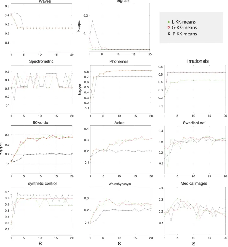
3.2.2. Experiment 1b: the parameter s

The parameter s is essential for the performance of the

KK-means algorithms. Small values of the parametersreduce the

com-putational cost, but too small values could lead to information being lost and computational performance being damaged. To analyze this issue KK-means algorithms have been run on test problems,

analyzing the value of the concordance coefficient

κ

versus the

parameter s¼1;…;20. The results are shown in Fig. 5. It is

generally observed that the maximum performance of KK-means algorithms is achieved by small values ofsshowing that it is a viable

strategy to reduce the dimensionality. Note that inWavesexample

the original classification arranges the data asy1;y2;y3whereas

KK-means algorithms use the functionsh1;h2;h3as category systems.

This means that when the parametersincreases this discrepancy is

enhanced.

3.2.3. Experiment 1c: perfomance of the approximate Kernel K-means

The essential difference between the kernel clustering methods proposed in the literature and the one developed in this paper is that they ignore the datafxig(ignore functional nature) and work directly with the data pointsfyi_gN

i¼1whereyiAR

n

. Unliked2_ϕand

d2Vn, the kernel distance function is computed as

d2Kðyi;yjÞ≔Kðyi;yiÞþKðyj;yjÞ2Kðyi;yjÞ ð32Þ whereKð⋯;Þ:RN_RN_{↦Ris a kernel function.}

We have focused the study on the aKKm algorithm because this algorithm achieves better clustering performance than the tradi-tional low rank kernel approximation and the running time and

memory requirements are significantly lower than those of kernel

K-means. Appendix A shows how the aKKm algorithm can be

derived by applying theK-means algorithm on a transformation of

the original data.

The aKKm algorithm samplesm5Npoints to approximate the

kernel matrix Ky _ij¼Kðyi;yjÞ. The parametermplays the role of

data reduction, the same role as the parametersin the KK-means

algorithms. We have repeated Experiment 1a using the valuem¼s

and Laplacian, Gaussian and polynomial kernels. As the data are now fyi_gN

i¼1 instead of fxigni¼1 they have different orders of

magnitude and it is necessary to calculate suitable parameters

for these algorithms. The parameters used are shown inTable 3.

Table 4

Value ofsused in test problems.

Problem s Problem s

Waves 10 Signals 10

Spectrometric 30 Phonemes 10

Irrationals 10 radar 20

50Words 20 Adiac 20

MedicalImages 20 SwedishLeaf 20

Synthetic-control 20 WordsSynonyms 20

Table 5

Kappa coefficient of agreementκ.

Problem K-means L-KK-means G-KK-means P-KK-means

Waves 0.263 0.260 0.263 0.253

Signals 0.010 0.010 0.010 0.010 Spectrometric 0.448 0.309 0.308 0.326 Phonemes. 0.824 0.818 0.821 0.701 Irrationals 0.150 0.425 0.525 0.525 50words 0.349 0.380 0.372 0.197

Adiac 0.319 0.319 0.308 0.190

MedicalImages 0.198 0.193 0.173 0.260 SwedishLeaf 0.313 0.326 0.305 0.324 Synthetic-control 0.482 0.482 0.590 0.650 WordsSynonyms 0.248 0.245 0.242 0.206

Table 6

Computational cost.

Problem K-means L-KK-means G-KK-means P-KK-means

Iter. p CPU (s) Iter. p CPU (s) Iter. p CPU (s) Iter. p CPU (s)

Waves 7.8 0.94 112.3 7.8 0.96 12.7 8.3 0.95 14.1 14.1 0.11 19.1

Signals 4.7 0.26 29.9 9.2 0.23 8.8 9.7 0.62 12.3 12.9 0.07 29.9

Spectrometric 7.4 1.0 25.4 7.4 0.70 11.8 7.5 1.0 14.1 9.7 0.79 14.6

Phonemes. 20.6 0.21 1188.4 24.9 0.002 163.6 23.7 0.29 166.2 23.2 0.34 59.9 Irrationals 13.1 0.001 5047.9 15.8 0.029 26.5 13.1 0.365 12.5 12.4 0.188 12.6 50words 22.3 0.001 4461.3 22.5 0.001 334.5 22.2 0.001 330.9 24.5 0.001 245.8 Adiac 36.8 0.001 2746.3 35.6 0.001 364.0 36.4 0.001 371.7 42.4 0.001 306.1 MedicalImages 31.1 0.003 582.9 30.1 0.001 132.2 30.7 0.001 145.5 32.9 0.002 117.6 SwedishLeaf 32.5 0.001 1246.9 30.9 0.001 219.3 32.3 0.001 194.6 39.1 0.001 219.7 Synthetic-control 11.8 0.067 46.6 11.5 0.007 21.2 11.5 0.048 22.1 13.3 0.001 22.8 WordsSynonyms 26.7 0.001 3080.3 26.6 0.001 216.1 26.9 0.001 217.1 30.9 0.001 174.3

The results obtained are displayed inTables 7 and 8. It can be observed that the performance of the algorithm is in general similar to KKmeans algorithms in almost all the problems. There

are only two significantly different problems. Theirrationals

problem, from not considering the functional natureaKKm, has a degree of concordance of almost 0. On the other hand the

Signals problem was not accurately addressed by the

KK-means methods. This is because the type of noise defines the

class in which each function is placed. Once an empirical function is projected, its noise is smoothed, and functions become indistinguishable from the KK-means algorithm. By contrast, the aKKm algorithm is able to identify the type of noise present in each signal.

3.3. Experiment 2: an application of functional cluster analysis for radar signals

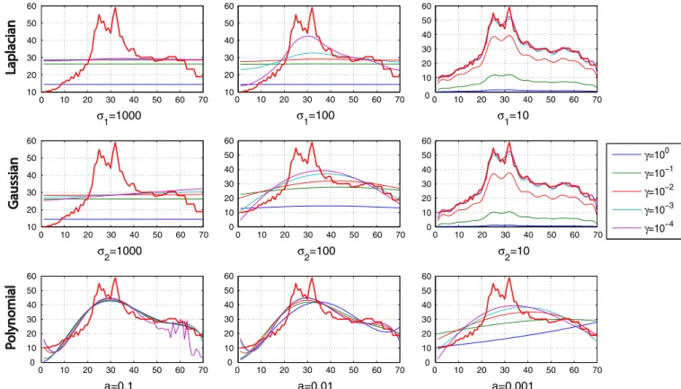
3.3.1. Computation of the kernel and its parameters

In this section we apply the proposed methodology to the real

Radarproblem. Thefirst task is to calculate the type of kernel, its parametrization and the regularization parameter

γ

. The expression

parameter b¼5 in all the experiments. The

γ

took the values 100;101;102;103and 104. The role that plays this parameter is shown clearly in Gaussian kernel with

σ

2¼10.“Great”values of

γ

for the determined problem lead the projection to take the shape of the original curve, but the norm of the projection is much smaller

than the norm of the original. Thus the parameter measurement

γ

involves taking

γ

-0þbut without causing an ill-posed system(7). A

polynomial kernel with a¼0.1 and

γ

¼104 exhibits an ill-posed

system. A visual inspection allows the choice of

σ

1¼

σ

2¼10 and

a¼0.01 and a regularization parameter

γ

¼104_{. We also note that}

Gaussian and Laplacian kernels produce similar projections and get results reproducing the average signal.

3.3.2. Determining the number of clusters

A second problem we must address to applyK-means algorithm

(for functional data or non-functional) is that the number of cluster

Kmust be known. Halkidi et al.[16]classify the validity methods in external, internal and relative methods. The external and internal are statistical methods based on Monte Carlo simulation. The relative methods choose a definedvalidity indexthat is optimized with respect to a Clustering Parametrization, in this case with

respect to the number of clustersK. In this numerical experiment

we have chosen three indexes representing different contexts. A

Xie-Beni index [35] has been applied to some fuzzy clustering

algorithms, the coefficient of determination for hierarchical cluster

analysis andF-Snedecor index for partitional methods such as the

K-means algorithm. We de_fine the following indexes:

1. Coefficient of determinationR2_{: This coefficient measures the} proportion of variance explained by the model. It is defined by

R2K¼1

SSKwithin

SStotal;

K¼2;…;Kmax ð33Þ

whereSSKwithinandSStotalare respectively the sum of squares in

K-clusters and the total sum of squares, that is,SS1within. This statisticR2K takes values inð0;1and its value can be a guide to choosing the number of clusters.

Wilks' Lambda Statistic is usually applied to multivariate analysis

of variance (MANOVA) and is associated with the coefficient of

determination by the expression R2_{¼1 Wilks’Lambda. The}

Wilks' Lambda Statistic has been applied to cluster analysis to

determine the number of clusters [20]. Kuo and Lin [20]

determine the value that gives a larger decreased of the statistic by visual inspection, in our case, a larger increased ofR2_{(that is,} a non-smooth point that looks like a sharp point).

2. F-Snedecor index: Analysis of covariance (ANCOVA) is a para-metric statistical method that tries tofind a significant differ-ence between the averages of certain groups but discounting the effects of the covariances (quantitative factors). Suppose we want to contrast the goodness of a statistical between Model 1 and another more complex model (with more parameters)

that we call Model 2. TheFstatistic can be written by

Fk2k1;Nk2¼

ðR22R 2

1Þ=ðk2k1Þ

ð1R22Þ=ðNk2Þ

; ð34Þ

wherek1andk2are the number of parameters estimated for

each of the models,R21andR 2

2are the coefficient of

determina-tion obtained with the models 1 and 2 respectively andNis the

number of observations. If we applied the above statistic to compare a partition withk1¼1 clusters to another withk2¼K,

the statistic would take the expression

IndexF¼ R

2

K=ðK1Þ ð1R2KÞ=ðNKÞ

: ð35Þ

Observe thatR21¼1ðSS 1

within=SStotalÞ ¼1ðSStotal=SStotalÞ ¼0. The motivation for using this index is found in the work of

Milligan and Cooper [27] which carried out an intensive

res-earch, based on Monte Carlo simulation analysis, for determining the correct number of clusters. They recommend maximizing the index

trðBÞ

K1

= tr_NðW_KÞ

: ð36Þ

TheBandWterms are the between and pooled within cluster

sum of squares and cross product matrices. Observe if we divide

the numerator and denominator of the index(36)by the total

sum of squaresSStotalwe obtain the index(35). 3. Xie-Beni index. It is defined by

IXB≔

∑N

j¼1∑Kk¼1ujkdðf j

;vk_Þ

Nminkaidðvk;viÞ

ð37Þ

Table 8

Computational cost.

Problem Laplacian aKKm Gaussian aKKm Polynomial aKKm

Iter. p CPU (s) Iter. p CPU (s) Iter. p CPU (s)

Waves 9.4 0.506 14.9 8.8 0.321 9.4 9.5 0.005 12.5

Signals 6.7 0.025 7.3 7.4 0.030 8.4 4.5 1.000 4.7

Spectrometric 7.6 0.012 9.5 6.9 0.363 6.2 6.2 0.757 5.4

Fonemes 17.1 0.464 41.4 16.3 0.160 35.5 21.4 0.107 51.0

Irrationals 7.5 0.002 13.6 17.5 0.001 33.5 5.5 0.394 9.8

50words 24.4 0.001 316.8 22.7 0.001 307.9 23.7 0.001 326.1

Adiac 35.0 0.001 246.5 24.5 0.001 179.0 32.1 0.001 279.2

MedicalImages 28.6 0.004 120.7 24.2 0.004 84.9 31.7 0.003 128.2

SwedishLeaf 29.0 0.001 151.6 25.6 0.001 120.3 33.4 0.001 208.3

Synthetic-control 11.0 0.004 22.6 9.7 0.058 21.6 11.6 0.002 25.8

WordsSynonym 28.4 0.001 211.6 27.1 0.001 201.5 26.6 0.001 198.3

p: estimate of the probability the method will reach the global optimum. Iter.: the mean number of iterations. Table 7

Kappa coefficient of agreementκfor aKKm.

Problem Laplacian aKKm Gaussian aKKm Polynomial aKKm

Waves 0.247 0.263 0.340

Signals 0.490 0.730 0.020

Spectrometric 0.154 0.328 0.448

Fonemes 0.781 0.839 0.466

Irrationals 0.010 0.010 0.010

50words 0.355 0.351 0.355

Adiac 0.246 0.359 0.329

whereujk¼1 if the elementjbelongs to clusterkand takes the value 0 otherwise,vi_{are the centroid of the clusters andf}j_the original data.

Fig. 7shows the coefficient of determinationR2_{and theFand}

Xie-Beni indexes. The first observation is that K-means,

L-KK-means and G-KK-L-KK-means algorithms have a similar behavior,

different from the behavior of the P-KK-means algorithm. TheF

and Xie-Beni indexes would take 2 clusters but there is little difference between 2 and 3 clusters. If we look at the coefficient of

determination R2 we find that K¼3 has a sharp point

(non-smooth). This criterion is used to determine the number of

clusters, the one that produces an abrupt change (that leads to the appearance of a sharp point). In addition, the value ofR2_{can be} used as a selection criterion because it can be explained as the square of the proportion of variance. For 2 and 3 clusters we obtain

R2 _{0:4 andR}2 _{0:5, respectively. Finally taking into account the}

above considerations we chooseKn¼3.

Fig. 8 shows the solution found by G-KK-means for Kn¼3

clusters. The cluster 1 contains 94 signals, the cluster 2 has 47 signals and the third cluster has 329. The projected curves are in the

left column and the original curves in the right.Fig. 9shows the

centroids (on the left the average of the projections and on the right the average of the original signals).

Fig. 6.Average projection for different kernels and parameters of theRadarproblem. (For interpretation of the references to color in thisfigure caption, the reader is referred to the web version of this article.)

4. Conclusions

In this paper we have addressed the problem of cluster analysis for

functional data. The proposed algorithm of K-means carried out by

this work, named KK-means, solves two important challenges: (i) it is

applicable to function domains where it is not possible to control the discretizationfxigni¼1 of the functions and (ii) these discretizations

lead to high dimensional problems due to the functional nature of the data and need strategies to reduce their dimensionality, in such a way that the performance of the procedure cluster is not reduced. Fig. 8.Solution found in theRadarproblem with G-KK-means. The curves in the left column are the projection and in the right column are the original curves.

The metricsdVnanddϕbased on projections onto Reproducing

Kernel Hilbert spaces (RKHS) and the Tikhonov regularization theory have been used. We have shown that both metrics are equivalent, however they lead, due to their nature, to two different strategies for reducing the dimension of the problem. In the case ofdVnthe most suitable strategies are Johnson–Lindenstrauss-type

random projections. The dimensionality reduction ford_ϕis based

on spectral methods.

In the numerical study we have given an exampleex professoto

show that if the samplingfxigni¼1 is not uniform inXa K-means

algorithm that ignores the functional nature of the data can reduce its performance. We have show numerically that for examples

where X is sampled uniformly the performance of the original

K-means algorithm and the aKKm algorithm is similar to the one

proposed but the computational cost, when working with the set of original data, is larger than the KK-means algorithm based ond_ϕ

or alternatively aKKm algorithm, because both algorithms use dimensionality reduction strategies.

It has been numerically proven that small values of the parameter

s, less than 20;allow for maximum performance of the algorithms. We have illustrated this methodology with a real problem to analyse what problems must be faced by the KK-means algorithm.

For real functions of a single real variable the expression (17)

allows a graphical representation that guides the choice of the

kernel type, its parameters and the regularization parameter

γ

.

Determining the correct number of clusters is a hard task.

Relying on a unique index can be misleading.R2_{is a good tool as}

it measures the proportion of variance and therefore choosing the minimum number of clusters to reach a specific value ofR2can be a good criterion. The good thing about methods based on projections is that they eliminate data noise and allow a better estimation ofR2_.

Acknowledgements

The authors wish to acknowledge financial support from

Ministerio de Economía y Competitividad under Project TRA2011-27791-C03-03.

The authors express their gratitude to the anonymous referees, the associate editor and the editor whose comments greatly improved this paper.

Appendix A. Relationships between functional principal component analysis anddVnanddϕ

FPCA is a tool which represents curves in a function space of reduced dimension. In this appendix we show the relationship between FPCA and the projections used in this paper. In this appendix, we follow the description of FPCA for time series (which is more restrictive than the case discussed in the paper) by Jacques and Preda[17]. We assume that for a time seriesf(t) theL2continuous stochastic process holds 8tA½0;T; lim

h-0E½ðfðtþhÞfðtÞÞ

2 _{¼0: ð38Þ}

Let

μ

ðtÞ ¼E½fðtÞ be the mean function and the covariance operator

Voff:

V:L2ð½0;TÞ↦L2ð½0;TÞ

g-VðgÞ≔ZT

0

Vð;tÞgðtÞdt

is an integral operator with kernelVdefined by

Vðs;tÞ ¼E½ðfðsÞ

_μ

ðsÞÞðfðtÞ

_μ

ðtÞ; s;tA½0;T: ð39Þ The spectral analysis ofV provides a countable set of positive eige-nvaluesf

_λ

jgjZ1associated with an orthonormal basis of eigenfunctions

ffjgjZ1. Theprincipal componentsfCjgjZ1 off(t) are random variables

defined as the projection offon the eigenfunctions ofV:

Cj¼ Z T

0

ðfðtÞ

_μ

ðtÞÞfjðtÞdt: ð40Þ

The Karhunen–Loeve expansion holds

fðtÞ ¼

_μ

ðtÞþ∑ jZ1

CjfjðtÞ; tA½0;T: ð41Þ

Truncating(41)at thefirststerms one obtains the best approximation in normL2off(t) by

fðsÞðtÞ ¼

μ

ðtÞþ ∑s j¼1

CjfjðtÞ; tA½0;T: ð42Þ

The computational methods for FPCA assume that the functional data

belong to a finite dimensional space expanded by some basis of

functions. Let

α

i¼ ð

α

i1;…;

α

iLÞT be the expansion coefficient of the observed curvebfiin the basis

Φ

¼ f

φ

1;…;

φ

Lgsuch that

b

fiðtÞ ¼

Φ

ðtÞT

α

i ð43Þ with

Φ

ðtÞ ¼ ð

φ

1ðtÞ;…;

φ

LðtÞÞ

T

:

LetA~ be theNL-matrix whose rows are the vectors

α

T

i, let

A¼ ðIN1Nð1=N;…;1=NÞÞA~ where IN and 1N are respectively the

identity NN-matrix and the unit column vector of size N and

W¼RT

0

Φ

ðtÞ

Φ

ðtÞ

T_{dt is the symmetric LL matrix of the inner}

products between the basis functions. The functional principal component analysis is reduced to the usual PCA of the matrixAW1=2. The eigenfunctionfjbelongs to the linear space spanned by the basis

Φ

:

fjðtÞ ¼

Φ

ðtÞTbj ð44Þ

withbj¼ ðbj1;…;bjLÞT

The principal component scores are given by

Cj¼AWbj: ð45Þ

We now compare the FPCA with the KK-means algorithms. Observe that the principal components have zero mean whereas the projectionsfnðxÞonto RKHS do not assume this condition. Operation-ally this means that working with the coefficient matrixAin the FPCA and withA~ in the case of the paper. If we translate the data thendVn

andd_ϕare preserved. The use ofAinstead ofA~ is equivalent to the translation of data to the origin and both approaches are equivalent.

To interpret dVn under the FPCA, consider the basis

φ

jðtÞ≔

Kðt;xjÞwithxjAXn. In this case,Theorem 1(a) guarantees

W¼Kx¼UTU)W1=2¼U: ð46Þ

By using FPCA, thefirst principal components ofAW1=2¼AUare

calculated. The distancedVnuses the transformation of the dataAU

as equivalent to considering all the principal components and working with the basisfKð;xjÞgxjAXn.

To interpretd_ϕ, we assume that the analytical expression for

the kernelVisKand consider

φ

j¼

ϕ

j the elements of the basis. Sinceffjgis an orthonormal basis forL2ð½0;TÞwe have

fj¼ ffiffiffi

λ

p

j

ϕ

j)bj¼ ð0;…; ffiffiffi

λ

p

j;…;0ÞT ð47Þ

and therefore the principal component is calculated

Cj¼AWbj¼A

1

λ1 0 ⋯ 0

0 1

λ2 ⋯ 0

0 0 ⋯ 1

λs 0 B B B @ 1 C C C Abjffi

ffiffiffi n p A 1_ffiffiffiffi ℓ1

p _{0 ⋯ 0}

0 1_ffiffiffiffi

ℓ2 p _{⋯ 0}

0 0 ⋯ 1_ffiffiffiffi

ℓs p 0 B B B @ 1 C C C Aej

¼pffiffiffinADs1=2ej ð48Þ

whereejis a vector whose components are all zero except for the

j-th component which is equal to one. This proves that the d_ϕ

There are two novel aspects with respect to the classical FPCA.

Thefirst issue is that the expansion(43)is performed using the

Tikhonov regularization theory. The second one is to interpret Euclidean distance between feature vectors (the principal compo-nents) as the distance between the projected functions.

Appendix B. Approximate kernelK-means (aKKm)

The purpose of this appendix is to show how the aKKm

algorithm can be obtained by applying the algorithmK-means to

a transformation of the original data. The main idea of these methods is the so-calledkernel trick, which allows inner products

to be computed in some, possibly in_finite-dimensional, feature

space. These methods are based on a nonlinear mapping

Ψ

ðÞ which projects the data representation in the original space onto thefeature spaceH. AMercer kernel Kð;Þ:YY↦Rallows us to

evaluate an inner product in thefeature spaceby the expression:

Kðyi;yjÞ ¼D

Ψ

ðyiÞ;

Ψ

ðyjÞE

H ð49Þ

whereh i;_H denotes the inner product inH.

The aKKm randomly samples mdata points m5N, denoted

by Yb¼ fby1;…;ybmg and construct a subspace Hb¼span½

Ψ

ðyb

1

Þ;

…;

Ψ

ðybmÞ. The kernel distance in the spaceHbis computed by

d2_H

bðy

k

;ys_Þ

≔ckðÞcsðÞ;ckðÞcsðÞ_H

b¼ ð

α

k

α

sÞ

T_Kb_ð

_α

k

α

sÞ ð50Þ

where

ckðÞ ¼ ∑ m

i¼1

α

kiKðyb i

;Þ;csðÞ ¼ ∑ m

i¼1

α

siKðby i

;Þ and Kbij¼Kðby i

;byjÞ

ð51Þ

Assuming the matrixKbis well-conditioned2_{and using the Cholesky}

decomposition b

K¼UTU:

The expression(50)can be calculated with Euclidean inner product

d2_H

bðy

k_;ys_{Þ ¼ U}

_α

kU

α

s;U

α

kU

α

s

2 ð52Þ

Chitta et al.[8]show that the relationship between the original data and the projections is given by

α

k¼Kb 1

φ

T

k ð53Þ

where

φ

k is the e k-th row of the matrix KBARNm which is

defined byKBði;jÞ ¼Kðyi;by j Þ.

Finally the above clustering method is equivalent to applying

theK-means algorithm (Euclidean distance) to the transformed

data (in rows)

KBKb 1

UT¼KBU1ðUTÞ1UT¼KBU1: ð54Þ

References

[1]C. Abraham, P.A. Cornillon, E. Matzner-Løber, N. Molinari, Unsupervised curve clustering using B-splines, Scand. J. Stat. 30 (3) (2003) 581–595.

[2]N. Aroszajn, Theory of reproducing kernels, Trans. Am. Math. Soc. 68 (3) (1950) 337–404.

[3]G. Biau, L. Devroye, G. Lugosi, On the performance of clustering in Hilbert spaces, IEEE Trans. Inf. Theory 54 (2) (2008) 781–790.

[4]L. Breiman, J. Friedman, R. Olshen, C. Stone, Classification and Regression Trees, Wadsworth, Belmont, CA, 1984.

[5]B. Cadre, Q. Paris, On Hölderfields clustering, Test 21 (2) (2012) 301–316. [6]J. Carletta, Assessing agreement on classification tasks: the kappa statistic,

Comput. Linguist. 22 (1996) 249–254.

[7]D.-R. Chen, H. Li, On the performance of regularized regression learning in Hilbert space, Neurocomputing 93 (2012) 41–47.

[8] R. Chitta, R. Jin, T.C. Havens, A.K. Jain, Approximate kernel K-means: solution to large scale kernel clustering, in: Proceedings of the 17th ACM SIGKDD International Conference on Knowledge Discovery and Data Mining, San Diego, California, USA, 2011, pp. 895–903.

[9]C. Cortes, V. Vapnik, Support-vector networks, Mach. Learn. 20 (3) (1995) 273–297. [10]D. Cox, F. O'Sullivan, Asymptotic analysis of penalized likelihood and related

estimators, Ann. Stat. 18 (1990) 1676–1695.

[11]F. Ferraty, P. Vieu, Nonparametric Functional Data Analysis, Springer Series in Statistics, Springer, New York, 2006.

[12]M. Filippone, F. Camastra, F. Masulli, S. Rovetta, A survey of kernel and spectral methods for clustering, Pattern Recognit. 41 (1) (2008) 176–190.

[13]C. Fyfe, P. Lai, Kernel and nonlinear canonical correlation analysis, Int. J. Neural Syst. 10 (5) (2001) 365–377.

[14]M. Girolami, Mercer kernel-based clustering in feature space, IEEE Trans. Neural Netw. 13 (3) (2002) 780–784.

[15] J. González-Hernández, Representing Functional Data in Reproducing Kernel Hilbert Spaces with Applications to Clustering, Classification and Time Series Problems (Ph.D. thesis), Department of Statistics, Universidad Carlos III, Getafe, Madrid, 2010.

[16]M. Halkidi, Y. Batistakis, M. Vazirgiannis, On clustering validation techniques, J. Intell. Inf. Syst. 17 (2-3) (2001) 107–145.

[17] J. Jacques, C. Preda, Functional Data Clustering: A Survey, Research Report, No. 8198, INRIA, 2013.

[18] E. Keogh, Q. Zhu, B. Hu, Y. Hao. X. Xi, L. Wei, C.A. Ratanamahatana, The UCR Time Series Classification/Clustering Homepage: www.cs.ucr.edu/ eamonn/ time_series_data/, 2011.

[19]G. Kimeldorf, G. Wahba, A correspondence between Bayesian estimation on stochastic processes and smoothing splines, Ann. Math. Stat. 41 (2) (1970) 495–502. [20]R. Kuo, L. Lin, Application of a hybrid of genetic algorithm and particle swarm optimization algorithm for order clustering, Decis. Support Syst. 49 (4) (2010) 451–462.

[21]J.Łȩski, A. Owczarek, A time-domain-constrained fuzzy clustering method and its application to signal analysis, Fuzzy Sets Syst. 155 (2005) 165–190. [22]T.W. Liao, Clustering of time series data- a survey, Pattern Recognit. 38 (2005)

1857–1874.

[23]L. Lovász, M.D. Plummer, Matching Theory, vol. 367, American Mathematical Society, Chelsea Publishing, Providence, 2009.

[24]J. MacQueen, Some methods of classification and analysis of multivariate observations, in: L.M. Le Cam, J. Neyman (Eds.), Proceedings of the Fifth Berkeley Symposium on Mathematical Statistics and Probability, vol. 1, University of California Press, Berkeley, CA, 1967, pp. 281–297.

[25]J. Mercer, Functions of positive and negative type and their connection with the theory of integral equations, Philos. Trans. R. Soc. Lond. Ser. A 209 (1909) 415–446.

[26] S. Mika, G. Rätsch, J. Weston, B. Schölkopf, K.-R. Müller, Fisher discriminant analysis with kernels. in: Proceedings of the IEEE International Workshop on Neural Networks for Signal Processing, Madison, USA, 1999, pp. 41–48. [27]G. Milligan, M. Cooper, An examination of procedures for determining the

numbers of clusters in a data set, Psychometrika 50 (1985) 159–179. [28]J. Peng, H.-G. Müller, Distance-based clustering of sparsely observed

stochas-tic, processes with applications to online auctions, Ann. Appl. Stat. 2 (3) (2008) 1056–1077.

[29]J.O. Ramsay, B. Silverman, Functional Data Analysis, Springer, New York, 2006. [30]B. Schökopf, A. Smola, K.-R. Müller, Nonlinear component analysis as a kernel

eigenvalue problem, Neural Comput. 10 (5) (1998) 1299–1319.

[31] B. Schölkopf, R. Herbrich, A.J. Smola, A generalized representer theorem, in: Proceedings of the Annual Conference on Computational Learning Theory, 2001, pp. 416–426.

[32] S. Smale, D.X. Zhou, Geometry on Probability Spaces, Working Paper, 2007. [33]D. Steinley, K-means clustering: a half-century synthesis, Br. J. Math. Stat.

Psychol. 59 (1) (2006) 1–34.

[34]A. Tikhonov, V.Y. Arsenin, Solutions of Ill-Posed Problems, Wiley, New York, 1997. [35]X.L. Xie, G. Beni, A validity measure for fuzzy clustering, IEEE Trans. Pattern

Anal. Mach. Intell. 13 (8) (1991) 841–847.

[36] W. Xu, X. Liu, Y. Gong, Document clustering based on non-negative matrix factorization, in: Proceedings of the SIGIR, 2003, pp. 267–273.

[37]G. Yao, W. Hua, B. Lin, D. Cai, Kernel approximately harmonic projection, Neurocomputing 74 (17) (2011) 2861–2866.

María Luz López Garcíais an Assistant Professor of Applied Mathematics at the University of Castilla-La Mancha. She received her M.Sc. degree in Mathematics from theUniversidad Autónoma de Madrid, Spain, in 1990 and a Ph.D. from theUniversidad de Castilla-La Mancha, Spain, in 2013. Her current research interests include data mining applied to transportation systems and artificial intelligence.

2

If the matrixKb had ill-conditioned problems, it could be replaced with

Ricardo García-Ródenasis an Assistant Professor of Applied Mathematics at the University of Castilla-La Mancha. He received a Mathematics degree from the

Universidad de Valencia, Spain, in 1991 and a Ph.D. from theUniversidad Politécnica de Madrid, Spain, in 2001. His current research interests include operational research in transportation systems and artificial intelligence.

Antonia González Gómezis an Assistant Professor of Applied Mathematics at theUniversity Politécnica de Madrid. She received a Mathematics degree from the