ENVIRONMENTAL ASSESSMENT OF LOW SPEED POLICIES FOR MOTOR
VEHICLE MOBILITY IN CITY CENTRES
J. CASANOVA1, * 1Department of Energy and Fluid Mechanical Engineering
N. FONSECA2 Universidad Politécnica de Madrid
2Department of Energy Systems
Universidad Politécnica de Madrid
Received: 16/12/11 *to whom all correspondence should be addressed:
Accepted: 09/03/12 e-mail: [email protected]
ABSTRACT
In order to assess the influence of reducing the speed limit from 50 km h-1 to 30 km h-1 in one-lane streets in local residential areas in large cities, real traffic tests for pollutant emissions and fuel consumption have been carried out in Madrid city centre. Emission concentration and car activity were simultaneously measured by a Portable Emissions Measurement System. Real life tests carried out at different times and on different days were performed with a turbo-diesel engine light vehicle equipped with an oxidizer catalyst and using different driving styles with a previously trained driver.
The results show that by reducing the speed limit from 50 km h-1 to 30 km h-1, using a normal driving style, the time taken for a given trip does not increase, but fuel consumption and NOx, CO and PM emissions are clearly reduced. Therefore, the main conclusion of this work is that reducing the speed limit in some narrow streets in residential and commercial areas or in a city not only increases pedestrian safety, but also contributes to reducing the environmental impact of motor vehicles and reducing fuel consumption. In addition, there is also a reduction in the greenhouse gas emissions resulting from the combustion of the fuel.
KEYWORDS: pollutant emissions, fuel consumption, motor vehicle, urban traffic calming.
INTRODUCTION
In order to increase pedestrian safety levels, in many urban residential zones of European cities, the speed of road motor vehicles has been limited to 30 km h-1 in narrow, local one-lane streets. Area-wide urban traffic calming schemes are to be implemented in many other residential zones to reduce the safety problems caused by road traffic. (Elvik 2001) reported a 25 % reduction in injury accidents when traffic is calmed but similar conclusions can be drawn for 30 km h-1 urban zones because at collision speeds below 30 km h-1, encounters between motor vehicles and pedestrians do not usually
result in a fatality.
But it is of great interest for urban authorities to assess whether such speed limits also have a positive effect on the environmental impacts of urban traffic and on transport energy consumption (as well as CO2 emissions). The answer to such a question is not as obvious as might be thought,
because the engine operating conditions at such low speeds might not be the best for low pollutant emissions and for fuel efficiency, and also the time spent in an urban journey might be increased This paper presents some experimental results regarding the expected changes to light diesel vehicle exhaust pollutant emissions and fuel consumption when the speed limit is reduced from 50 km h-1 to 30 km h-1 in some narrow urban streets, but not in other arterial or collector streets of the
same district, with more than one lane.
It is well known that motor vehicle exhaust emissions (CO, HC, NOX and PM) are a significant
In Europe, all light vehicles have to fulfil restrictive emissions limits that are certified by tests carried out in chassis dynamometers, in which the vehicle is driven following an NEDC (New European Driving Cycle) driving pattern comprising an urban cycle with 50 km h-1 as maximum speed and an extra-urban cycle with 120 km h-1 as the maximum speed. Although in the certification test there are speeds as slow as 30 km h-1, the emissions and fuel consumption at such speeds are not recorded
on their own. Several research studies on vehicle emissions carried out in real life urban traffic conditions have shown that real emissions are quite different from certified emissions for a given car (Lenaers, 1996; Pelkmans, 2006) and that this issue is much more important in the case of slow speeds.
The speed, the acceleration and the street slope significantly affect the fuel economy and the pollutant emissions of a vehicle during a trip through the city (Daham et al., 2005, Li et al., 2006, Li et al., 2007; Li et al., 2010). The power used, the transitory condition and the rotational speed of the engine at each instant result in the instantaneous fuel consumption and emissions of each pollutant during a given trip. During a complete trip through a city, the resulting total mass of pollutants emitted and the fuel consumed is not only a consequence of the average speed and acceleration, but also of the instantaneous engine conditions, which is a function of the driving style (De Vlieger 2000). It is expected that by reducing the maximum speed in some streets of a city, both the average speed and accelerations will also be reduced. But it could be the case that the operating point of the engine when the speed is very low could be a low efficiency point or a high emission point. It should be noted that some correlations of fuel consumption with average speed, regarding fuel consumption and emissions inventories, show an increase in both emissions and fuel consumption factors when the average speed is reduced in the range that occurs in urban areas (less than 40 km h-1) (Fonseca et al., 2010). This trend cannot be applied to the case to be studied, because it is related to similar speed limitations and to speed reductions that are mainly due to traffic conditions and to more intersections and stops per kilometre. However, this is not the case when dealing with different speed limitations and the same number of intersections and stop lights.
In order to assess the influence of reducing the speed limit from 50 to 30 km h-1 in one-lane streets in local residential zones of a large city, emissions and fuel consumption have been measured in real traffic tests following a representative route along the narrow streets of a typical central district of Madrid. In such a district, there are both one-lane streets that are likely to be included in 30 km h-1 zones and arterial streets with more than one lane.
It might be thought that less speed implies more time driving the car and consequently more time with the engine running, which could lead to more pollutants emitted into the atmosphere and more fuel consumed; however, this is not the case. A lower maximum speed is only expected to slightly change the average speed but not the acceleration values and acceleration time, which are expected to be the main periods with high values of fuel consumed and pollutants emitted. So, one of the aims of this work was to assess this predicted behaviour.
Therefore, this paper presents the results obtained with a light duty diesel vehicle that is representative of common medium size passenger cars in Europe, when travelling through the above-mentioned urban zones. A new car was not used because the purpose of the tests was to collect data on real-life cars circulating in European cities.
An on-board Portable Emissions Measurement System developed and validated in various tests by the authors for light duty cars (Fonseca and Casanova, 2009), was the main instrument used in this research to measure fuel consumption, car activity and environmental parameters instantaneously in real traffic emission conditions.
EXPERIMENTAL ASPECTS On-board instrumentation
The Portable Emissions Measurement System (PEMS), called MIVECO–PEMS 2.0, used in these tests is a combination of different exhaust gas analyzers, measuring systems for thermodynamic variables and meteorological and car parameters as well as recording and energy supply systems. It comprises the following parts:
−
Sampling tube and exhaust flow-meter, which includes a Pitot type flow-meter specially designed for hot and wet exhaust gases, with NOX and O2 chemical cells and absolute pressure andtemperature sensors.
−
A frame containing a CO and CO2 NDIR (Non Dispersive Infrared) analyzer, heated HC FID(Flame Ionization Detector) analyzer, a laser spectrometry mass PM analyzer and all the amplifiers and electronic units. It also includes the vacuum pumps and a gas cooling Peltier unit. (Fonseca and Casanova, 2009).
−
A system for recording the temperature, the pressure and speed of the surrounding air.The measurement system was powered by two lead acid batteries. A laptop was used to control and record the different instruments. Figure 1 shows a scheme of the on-board instrumentation.
Lambda meter ETAS LA4
EXHAUST
GASES Sampling tube
Peltier air cooler
T
Differential pressure
sensor
Filter HC analyzer ThermoFID PT
PM analyzer MAHA MPM-4 NO / NO2analyzer SENSORS NDUV BENCH NOX& O2analyzer
HORIBA MEXA 720
CO / CO2analyzer SIGNAL 9000
C
o
ld s
a
m
p
le
line
Pitot tube
Sample tube
External instrumentation
Engine instrumentation
RPM sensor Centralauto TB8600
Oil temperature
Cooling water temperature
GPS HAICOM-206
Weather station SKYWATCH GEOS 11
Data acquisition system RADAR Doppler GHM Engineering DRS1000
∆p
Flow meter
MIVECO
Heat
ed
samp
le l
in
e
Exhaust gases measurement systems
Figure 1. Portable emissions and car activity measurement system for on-board measurements
The recorded signals are post-processed to obtain instantaneous and averaged results of the emission factors (g km-1) and fuel consumption in litres per 100 km.
In order to calculate the instantaneous pollutantat the instant “i” mass flow emission (m j,i) for each pollutant, Eq. 1 was used:
i i i i
j,i j,i 6 E,i
E E E
ppmV M g /mol
m g/s ·m g/s ·
M g /mol 10
⎡ ⎤
⎡ ⎤
= χ
⎡ ⎤ ⎡ ⎤ ⎢ ⎥
⎣ ⎦ ⎢ ⎥ ⎣ ⎦
⎣ ⎦ ⎣ ⎦
(1)
whereχj,i is the instantaneous molar fraction of pollutant “j”. mE,i is the instantaneous exhaust mass flow calculated as the instantaneous exhaust volume flow (measured by the Pitot type flow-meter) multiplied by instantaneous exhaust gas density. Mi and ME are the pollutant “j” and exhaust gas
molar mass respectively. The fuel used was commercial diesel-oil following the European Standard EN 590. It contained almost 4 % of biodiesel. The fuel consumption was computed from the instantaneous lambda factor (λi) measured directly on exhaust flow and using the CHO formulae of
an excellent correlation being obtained. Eq. 2 was used to calculate the instantaneous fuel mass flow (mF,i), where (A/F)EST is the stoichiometric air fuel ratio.
E,i F,i
i
EST
m g
m
s A
1
F
⎡ ⎤
= ⎢ ⎥
⎣ ⎦ ⎛ ⎞
+ λ ∗ ⎜ ⎟⎝ ⎠
(2)
Global emissions and fuel consumption factors (EFj and FCF respectively) were calculated by
dividing the total mass amount of each pollutant or the mass of fuel consumed by the total distance travelled in each sector of the route and for each trial, as shown in Equations 3 and 4:
N j,i i 1
j N
i i 1
m g/s t s
s
EF g / km 3600
h v km/h t s
=
=
⋅ ∆
⎡ ⎤ ⎡ ⎤
⎣ ⎦ ⎣ ⎦ ⎡ ⎤
= ⋅
⎡ ⎤
⎣ ⎦ ⎢ ⎥⎣ ⎦
⋅ ∆
⎡ ⎤ ⎡ ⎤
⎣ ⎦ ⎣ ⎦
∑
∑
(3)
N F,i i 1
N
F i
i 1
m g/s t s
100 s
FCF l /100 km 3600
g/l h
v km/h t s
=
=
⋅ ∆
⎡ ⎤ ⎡ ⎤
⎣ ⎦ ⎣ ⎦ ⎡ ⎤
⋅ = ⋅ ⋅
⎡ ⎤
⎣ ⎦ ρ ⎡ ⎤ ⎢ ⎥⎣ ⎦
⎣ ⎦ ⋅ ∆
⎡ ⎤ ⎡ ⎤
⎣ ⎦ ⎣ ⎦
∑
∑
(4)
Where vi is the instantaneous car speed, ∆t is the sample time used for data register, N is the number of instantaneous data sampled in each trial and ρF is the fuel density.
Vehicle and driver
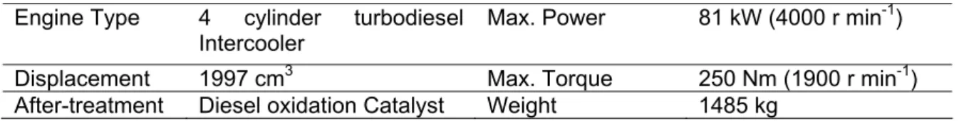
A light duty passenger car (Peugeot 406 2.0 HDI Break) was used for these tests. The main characteristics are shown in Table 1.
Table 1. Characteristics of the car used in the tests
Engine Type 4 cylinder turbodiesel
Intercooler Max. Power 81 kW (4000 r min
-1)
Displacement 1997 cm3 Max. Torque 250 Nm (1900 r min-1)
After-treatment Diesel oxidation Catalyst Weight 1485 kg
Obviously it was a used car, but the engine and the entire car were completely checked before the tests. Although it fulfilled the Euro 2 emissions limits, the technology used in this car to reduce pollutant emissions was similar to that used in most Euro 4 passenger cars, with a DOC (Diesel Oxidation Catalyst) and not a Diesel Particle Filter, which is the most widespread technology nowadays.
The vehicle driver was the same in all the tests, a normal driver who had held a driving licence for over 10 years. He had been previously trained in different normal, aggressive and Ecodriving trips. Three degrees of aggressiveness were used, in order to see the influence of the driver on the results:
−
Aggressive driving pattern, with high acceleration and deceleration values, but not exceeding the maximum speed.−
Normal driving pattern following the surrounding vehicles, maintaining normal smooth accelerations and decelerations when braking.Route
As the tests were focused on the effect of speed limits on emissions and fuel consumption, the routes had to include narrow one-lane roads but also wider roads with two or more lanes on each side. The function of the streets had to be residential or commercial, mainly local streets instead of collector streets.
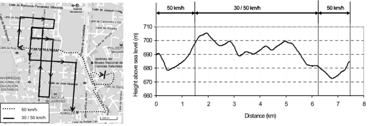
Taking these constraints into account, a route along the streets of the Chamberi district of Madrid was plotted including streets limited to 30 km h-1 or 50 km h-1 and also other streets limited to 50 km h-1. Neither ring roads nor motorways were included. Figure 2 shows the map of the route on the plan of the Chamberi district in Madrid and the slope profile of this route. It can be seen that Madrid is characterized by streets that are never flat. This strongly affects the average fuel consumption and emission factors of the cars in central urban zones.
50 km/h
30 / 50 km/h 200 m
50 km/h 30 / 50 km/h 50 km/h
30 / 50 km/h 200 m200 m
660 670 680 690 700 710
0 1 2 3 4 5 6 7 8
Distance (km)
H
ei
ght
abo
ve
sea
le
ve
l (
m
)
50 km/h 30 / 50 km/h 50 km/h
660 670 680 690 700 710
0 1 2 3 4 5 6 7 8
Distance (km)
H
ei
ght
abo
ve
sea
le
ve
l (
m
)
50 km/h 30 / 50 km/h 50 km/h
Figure 2. Map and slope profile of the route
Testing procedure
33 tests were conducted in three different driving styles; 12 normal and 12 eco-driving and aggressive. About 250 km were travelled that corresponded to about 15 hours of data collected each 0.1 seconds. The tests were randomly carried out during eight different days throughout the month of March 2011.
In the one-lane local streets in which these tests were made, the traffic flow is usually light because those streets are used mainly by local residents to access the main streets. This vehicle flow is naturally regulated by priority on street intersections; however, it is affected by random phenomena such as the stopping of a car to unload goods or persons or to park at the kerb. Despite the small variation in traffic during the day, tests were carried out during both peak and off-peak hours of the day to statistically eliminate any possible influence.
Emissions analyzers, heated line and sample tube heating were warmed throughout the night before the tests. A calibration procedure was carried out before each day of the tests, and the engine was heated during a previous 5 km route, and also to ensure that all systems were functioning properly. In addition, the sample tube was scavenged with hot air between each consecutive tests.
RESULTS AND DISCUSSION
Effect of speed limit on vehicle dynamics
The results are presented here as averaged values of dynamic variables of the car movement. The average results were computed from each trial, which included the car moving in a zone in which the speed was always limited to 50 km h-1 because there were more arterial than one-lane roads, and in another zone in which the speed was limited to 50 km h-1 or 30 km h-1 because they were narrow one-lane streets. It was attempted to reproduce the reality of a car driving along the streets of a standard city centre. The results set out here include only those where a normal driving style was used by the driver.
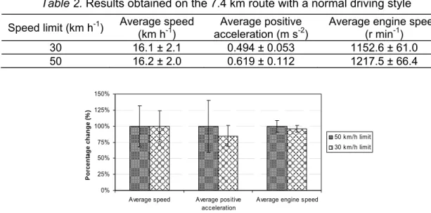
Table 2. Results obtained on the 7.4 km route with a normal driving style
Speed limit (km h-1) Average speed (km h-1) acceleration (m sAverage positive -2) Average engine speed (r min-1)
30 16.1 ± 2.1 0.494 ± 0.053 1152.6 ± 61.0
50 16.2 ± 2.0 0.619 ± 0.112 1217.5 ± 66.4
0% 25% 50% 75% 100% 125% 150%
Average speed Average positive acceleration
Average engine speed
P
o
rcen
ta
g
e
ch
an
g
e
(
%
)
50 km/h limit 30 km/h limit
Figure 3. Average speed, positive acceleration and engine speed for the total route
From Figure 3, it can observed that for the whole route that changing the speed limit in only one part of it does not affect the average speed of the whole route. Nevertheless, it can be seen that the average positive acceleration is reduced by 20 % and the average engine speed is slightly reduced by 5 % when the speed is limited to 30 km h-1. This means that the driver naturally increases the
speed more slowly when he tries to reach the 30 km h-1 limit than when he tries to reach the 50 km
h-1 limit. In fact, the car is always increasing or decreasing its speed, because the distance between street intersections is less than 200 m in the 30 – 50 km h-1 zone. The reason for those results can be explained in both cases by the analysis of the instantaneous driving pattern.
0 10 20 30 40 50
0 500 1000 1500 2000 2500
In
stant
a
n
e
ous Speed (
k
m/h)
Time (s)
Speed limit 30 km/h
Speed limit 50 km/h
Figure 4. Instantaneous speed on the same section of the route with 30 and 50 km h-1 speed limits
Figure 4 shows the instantaneous speed of the car on the same section of the route, with no traffic light-controlled street intersections. It can be observed that the speed is always changing due to the fact that street sections between intersections are short (approx. 100 m). For this reason, with the 50 speed limit the car never reaches the maximum speed, even though the driver presses the accelerator pedal more. When approaching an intersection the car speed is reduced and the car only stops if another car or pedestrian has the right of way.
Effect of speed limit on fuel consumption and pollutant emissions.
Figure 5 shows the instantaneous fuel consumption on the urban section of the route, in which the speed limit is changed from 50 km h-1 to 30 km h-1. In the acceleration periods the fuel consumption
0 1 2 3
0 500 1000 1500 2000 2500
In
s
tan
ta
neou
s fue
l
con
s
umptio
n (g/
s
)
Time (s)
Speed limit 50 km/h Speed limit 30 km/h
Figure 5. Instantaneous speed along the section of the urban route, with both speed limits
Peak fuel consumption of 1.8 to 2.2 g s-1 can be found at the 50 km h-1 limit, but this peak fuel consumption does not exceed 1 g s-1 at the 30 km h-1 limit. As a result of such instantaneous
behaviour, the accumulated fuel consumption along the whole section of the route is much lower, as the graph in Figure 6 shows for the same section of Figure 5.
0 25 50 75 100 125 150
0 500 1000 1500 2000 2500
A
c
c
u
mul
a
ted
fu
el
c
o
n
s
um
pt
io
n
(
g
)
Time (s)
Speed limit 30 km/h Speed limit 50 km/h
Figure 6. Accumulated fuel consumption along the same section of the urban route, with both speed limits
The pollutant emissions are also affected by the speed limit but in a different way. Figure 7 shows the relative change in NOX, CO, HC and PM mass emissions along the studied urban route that
includes 50 km h-1 limit zones and 30 – 50 km h-1 limit zones (Figure 2).
0% 50% 100% 150% 200%
Fuel consumption
NOx Emission factor
CO Emission factor
HC Emission factor
PM Emission factor
P
o
rc
ent
age c
hange (
%
)
50 30
Figure 7. Modification of emissions and fuel consumption in the studied urban route when the speed limit is reduced to 30 km h-1
Nitrogen oxides, carbon monoxide and particulate matter emissions are reduced when the speed limit is reduced to 30 km h-1, but hydrocarbon emissions increase. The increase in average HC emissions does not have any statistical significance due to the high variability observed. However, this variability can be explained because these emissions are formed in transient operating conditions that depend on several instantaneous engine conditions such as exhaust gas temperature, oxidation, catalytic converter temperature, fuel / air ratio, turbocharger conditions, etc., that are also a function of engine load and speed, as well as the time spent with the car stopped (cooling of the catalytic converter).
The reduction in NOX emissions, when the speed limit is reduced, is linked to the fuel consumption
reduction shown in Figures 5, 6 and 7, due to the fact that NOX emissions depend on the relative fuel
0,1 1
0 50 100 150 200 250
0 500 1000 1500 2000 2500
NO
X
em
si
si
on
(
p
p
m
V
)
Time (s)
NOx (ppmV) Fuel-air ratio
Re
la
tiv
e
fu
el
-ai
r ra
tio
Figure 8. Instantaneous NOX emissions related to relative fuel / air ratio
Table 3 shows the numerical values of the fuel consumption (l per 100 km) and emission factors (g km-1) along with the standard deviations of the different test trials on the same route. The fuel
consumption increase, as was previously explained, has a low standard deviation.
Table 3. Fuel consumption and emission factor on the urban route with both speed limits Speed
limit (km h-1)
Fuel consumption
(l 100km-1)
NOX emission
factor (g km-1)
CO emission factor (g km-1)
HC emission factor (g km-1)
PM emission factor (g km-1)
30 9.4 ± 0.5 0.65 ± 0.07 0.27 ± 0.17 0.012 ± 0.010 0.31 ± 0.15
50 11.1 ± 0.8 0.89 ± 0.44 0.34 ± 0.12 0.009 ± 0.006 0.40 ± 0.19
The reduction in the CO emission factor is due to the rise of the average catalytic converter temperature, which improves the catalytic converter oxidation performance. A 14 % rise in exhaust gas temperatures was measured.
Influence of driving style when speed limit is 30 km h-1
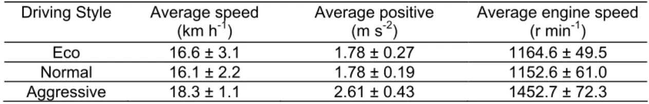
The driving style affects the above-explained results. In order to illustrate this influence, Figure 9 illustrates the percentage change in average speed, average positive acceleration and average engine speed when the car is driven in Ecodriving and Aggressive styles with respect to the Normal driving behaviour of the same driver.
0% 50% 100% 150% 200%
Average speed Average positive acceleration
Average engine speed
P
or
cent
age c
h
ange (
%
)
Eco Normal Agressive
Figure 9. Percentage change in average speed, positive acceleration and engine speed
during 30 km h-1 sections of the route with three driving styles
Table 4. Results of dynamic variables for the three driving styles for the route Driving Style Average speed
(km h-1) Average positive (m s-2) Average engine speed (r min-1)
Eco 16.6 ± 3.1 1.78 ± 0.27 1164.6 ± 49.5
Normal 16.1 ± 2.2 1.78 ± 0.19 1152.6 ± 61.0
Aggressive 18.3 ± 1.1 2.61 ± 0.43 1452.7 ± 72.3
Figure 10 illustrates the percentage change in fuel consumption factors and NOX, CO, HC and PM
emissions when Ecodriving and Aggressive driving styles are used with respect to the Normal driving styles that are presented in Table 5. The results for Fuel consumption and NOX emissions
follow the tendencies found in car and engine behaviour but other emissions follow different tendencies. CO and HC emissions are higher in Ecodriving conditions due to lower oxidation catalyst temperatures (a reduction of about 10 % in average exhaust gas temperature was measured). Higher CO emissions in aggressive driving are due to higher fuel / air ratios in transient acceleration periods and the lower HC emissions to higher oxidation catalyst temperatures.
0% 50% 100% 150% 200%
Fuel consumption
NOx Emission factor
CO Emission factor
HC Emission factor
PM Emission factor
P
o
rc
ent
age
chang
e (
%
)
Eco Normal Agressive
Figure 10. Percentage change in fuel consumption and emission factor during 30 km h-1 sections of the route with three driving styles
PM emissions mainly depend on engine load, and then the tendency for them to increase as the aggressiveness of the driving style increases is what would be expected. The high standard deviation of CO, HC and PM emissions is probably due to the transient operative conditions of the turbocharger, too far removed from its design operating conditions.
Table 5. Emission and fuel consumption results for the three driving styles Driving style FCF (l 100km-1) NO
X (g km-1) CO (g km-1) HC (g km-1) PM (g km-1)
Eco 9.3 ± 1.0 0.67 ± 0.12 0.39 ± 0.22 0.019 ± 0.012 0.24 ± 0.13 Normal 9.4 ± 0.5 0.65 ± 0.07 0.27 ± 0.17 0.012 ± 0.010 0.31 ± 0.15 Aggressive 12.2 ± 1.0 0.86 ± 0.18 0.44 ± 0.16 0.005 ± 0.004 0.52 ± 0.29
CONCLUSIONS
From the tests carried out in a light duty diesel vehicle driven along urban streets with two different speed limits, the following conclusions can be highlighted:
Reducing the speed limit in some residential narrow one-lane streets in city centres, which is being used to increase pedestrian safety, is also a good measure to reduce fuel consumption, and the resulting Green House Gas emissions.
Also CO, NOX and PM emission factors tend to be lower when the speed is limited to 30 km h-1
than when the limit is 50 km h-1, but on the other hand HC emissions are increased. But it is assumed that the most important pollutants in the case of European cities are NOX and PM,
mainly when dealing with diesel engine cars.
The driving style affects the results, which, in turn, affects the fuel consumption factors as well as the emission factors.
ACKNOWLEDGMENTS
The author wish to thanks Alexandre Baudry and Cesar Chacon for their help in preparing and carrying the tests, Jesus Rodriguez for processing the data and Adrian Alonso for driving the car during the road trials. The financial support of the Spanish Ministry of the Environment is gratefully acknowledged.
REFERENCES
Aarts L. and van Schagen I., (2006). Driving speed and the risk of road crashes: a review, Accident Analysis and Prevention, 2, 215-224.
Casanova J., Fonseca N. and Espinosa F., (2009). Proposal of a dynamic performance index to analyze driving pattern effect on car emissions. Proceedings 17th Transport and air pollution symposium and 3rd Environment and Transport Symposium. Toulouse, France. Actes INRETS n°122.
Casanova J., Margenat S., Ariztegui J., (2005). Impact of driving style on Pollutant Emissions and Fuel Consumption for Urban Cars. Proceedings of the 1st International Congress of Energy and Enviroment Engineering and Management. Potoalegre, Portugal. P.175.
Daham B., Andrews G., Li H., Ballesteros R., Bell M., Tate J. and Ropkins K., (2005). Application of a Portable FTIR for Measuring On-Road Emissions, SAE Technical paper, 2005-01-0676.
De Vlieger I. (1997). On board emission and fuel consumption measurement campaign on petrol-driven passenger cars, Atmospheric Environment,31(22), 3753-3761.
De Vlieger I., De Keukeleere D. and Kretzschmar J., (2000). Environmental effects of driving behaviour and congestion related to passenger cars, Atmospheric Environment,34(27), 4649-4655.
Elvik R., (2001). Area-wide urban traffic calming schemes; A meta-analysis of safety effects, Accident Analysis and Prevention, 33(3), 327-336.
Fonseca N. and Casanova J., (2009). Problemas asociados a la medida de emisiones másicas instantáneas en motores de vehículos. Memorias del VI Jornadas Nacionales de Ingeniería Termodinámica JNIT2009 ISBN 078-84-692-2642-1, Córdoba, España.
Fonseca N., Casanova J. and Espinosa F., (2010). Influence of Driving Style on Fuel Consumption and Emissions in Diesel-Powered Passenger Car, Transport and Air Pollution, 18th International Symposium TAP 2010, Zurich May 2010, 57-7.
Johansson H., Gustafsson P., Henke M., Resengren M., (2003). Impact of Ecodriving on emissions. 12th International Symposium "Transport and Air Pollution" Avignon, 16-18 june 2003 Proceedings actes, 92(1). Inrets ed., Arcueil. France, 2003. 113-120.
Lenaers G., (1996) On-board real life emission measurements on a 3 way catalyst gasoline car in motor way-, rural- and city traffic and on two Euro-1 diesel city buses, Sci Total Environ., 189/190,
139-147.
Li H., Andrews G., Daham B., Bell M., Ropkins K., (2006). Study of the Emissions Generated at Intersections for a SI Car under Real World Urban Driving Conditions, SAE Technical paper, 2006-01-1080.
Li H., Andrews G., Daham B., Bell M., Tate J., Ropkins K., (2007). The Impact of Traffic Conditions and Road Geometry on Real World Urban Emissions using a SI Car, SAE Technical paper 2007-01-0308.
Li H., Andrews G., Tate J., Ropkins K., Bell M., (2010). Driver Variability Influences on Real World Emissions at a Road Junction using a PEMS, SAE Technical paper, 2010-01-1072.
Pelkmans L. and Debal P., (2006). Comparison of on-road emissions with emissions measured on chassis dynamometer test cycles. Transportation Research Part D: Transport and Environment 11(4), July 2006, Pages 233-241.
Saboohi Y. and Farzaneh H., (2009). Model for developing an eco-driving strategy of a passenger vehicle based on the least fuel consumption, Applied Energy,86, 1925–1932.
Takada Y., Ueki S., Saito A., Sawazu N., Nagatomi Y., (2007). Improvement of Fuel Economy by Eco-Driving with Devices for Freight Vehicles in Real Traffic Conditions, SAE Technical paper, 2007-01-1323
Taylor M. and Wheeler A., (2000). Accidents reductions resulting from village traffic calming. In: Demand management and safety systems; proceedings of seminar J, Cambridge 11-13 September 2000, p. 165-174
Vis A.A., Dijkstra A. and Slop M., (1992). Safety effects of 30 km/h zones in The Netherlands, Accidents Analysis and Prevention, 24, 75-86.