Dislocation dynamics in non-convex domains using
finite elements with embedded discontinuities
Ignacio Romero , Javier Segurado and Javier LLorca
Departamento de Mecanica Estructural, Universidad Politecnica de Madrid, E. T. S. de Ingenieros Industrials, 28006 - Madrid, Spain
Departamento de Ciencia de Materiales, Universidad Politecnica de Madrid, E. T. S. de Ingenieros de Caminos, 28040 - Madrid, Spain
Instituto Madrileno de Estudios Avanzados en Materiales (IMDEA-Materiales), E. T. S. de Ingenieros de Caminos, 28040 - Madrid, Spain
Abstract
The standard strategy developed by Van der Giessen and Needleman (1995 Modelling Simul. Mater. Sci. Eng. 3 689) to simulate dislocation dynamics in two-dimensional finite domains was modified to account for the effect of dislocations leaving the crystal through a free surface in the case of arbitrary non-convex domains. The new approach incorporates the displacement jumps across the slip segments of the dislocations that have exited the crystal within the finite element analysis carried out to compute the image stresses on the dislocations due to the finite boundaries. This is done in a simple computationally efficient way by embedding the discontinuities in the finite element solution, a strategy often used in the numerical simulation of crack propagation in solids. Two academic examples are presented to validate and demonstrate the extended model and its implementation within a finite element program is detailed in the appendix.
1. Introduction
The understanding of microscale processes which control plastic deformation in engineering materials has been based, to a considerable extent, on relatively simple models. The expectations of nanotechnology—which have increased interest in the mechanical behavior of components at micrometer-scale—together with developments in modeling tools have led the way to more accurate and, to some extent, quantitative numerical simulations. In these analyses, the microstructural details at the micrometer and nanometer scale are explicitly taken into account to analyze the micromechanisms of deformation and fracture
most relevant strategies in this area and two different approaches have been developed. One of them mainly focuses on the analysis of physical micromechanisms of plastic deformation (dislocation interaction and multiplication, formation of dislocation structures, strain and forest hardening, etc) , while the microstructure and the boundary conditions are kept simple (e.g. an infinite single crystal subjected to homogeneous tension). The other is aimed at the solution of boundary value problems at the micrometer scale and includes the analysis of plastic deformation (and the associated size effects) during bending of small beams nanoindentation , uniaxial deformation of polycrystals , fracture of confined thin films , etc.
The solution of boundary value problems within the framework of discrete dislocation dynamics is a complex task which can only be accomplished, in general, through the combination of analytical results and numerical simulations. An important tool in studies of this kind is the model developed by Needleman and Van der Giessen , in which long-range interactions between individual dislocations are accounted for using the analytical expressions for the interaction between dislocations in an infinite and isotropic elastic solid. The effect of finite boundaries is included through another term for the stresses acting on each dislocation, which is computed by solving a complementary linear elastic boundary value problem using the finite element method with appropriate boundary conditions. The dislocation dynamics problem is solved in an explicit incremental way, using an Euler forward time-integration algorithm for the equations of evolution. This paper presents an extension of this methodology to deal with the effect of dislocations leaving the crystal through a free surface in the case of arbitrary non-convex domains, in which the intersection of the slip plane with the domain is not a continuous segment. The strategy used in the original framework to deal with dislocations leaving the domain was to place these dislocations in a fictitious position along its slip plane but far away from the domain and to include the deformation field induced by these dislocations (which is almost identical to the exact slip caused by the dislocation glide) to determine the total displacements of the domain. However, this method is not always applicable in the case of non-convex domains that contain defects with dimensions of the order of the Burgers vector (such as sharp cracks, very thin slits or nm voids) because the deformation field induced in the domain by a fictitious dislocation within the defect is very different from the actual one due to dislocation leaving the domain. Examples of these situations can be found in micro-electro-mechanical and micro-electronics devices or in the analysis of relevant topics in micromechanics such as cracked bodies, the growth of microvoids or the mechanical behavior of nanoporous metals . The new approach is based on the use of finite elements with embedded discontinuities following previous investigations
The outline of the paper is as follows. After the introduction, the main features of the Needleman and Van der Giessen model are briefly recalled with special emphasis on the case of dislocations leaving the domain. The new approach for non-convex domains is presented in section 3, while the numerical implementation using finite elements with embedded discontinuities is detailed in section 4. Two examples of application are presented in section 5 to validate and demonstrate the extended model and the paper ends with the conclusions section. An appendix is provided to facilitate the numerical implementation within the framework of the finite element method.
2. Basic discrete dislocation dynamics framework
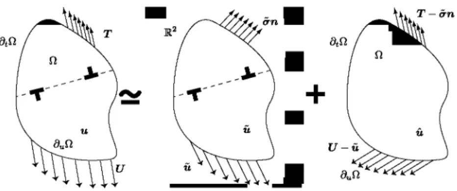
Figure 1. Problem decomposition. The problem in the center is posed on an infinite domain with the dislocations in it. The problem on the right is on the original domain 52, but the imposed tractions and displacement boundary conditions are corrected. The three problems in the figure will be denoted problems P, P and P, respectively.
gliding on one or more families of slip planes, each one characterized by the unit normal and tangent vectors, n and m, respectively. The crystal is assumed to remain in a state of plane strain at all times, and its cross section occupies a domain S c I2. The boundary 9£2 is partitioned into disjoint sets dtQ and duQ. Surface tractions T are applied on the former, and
displacements U are imposed on the latter. See figure 1 for an illustration of these definitions. The dislocations move on their slip planes, and their velocity can be accurately approximated using a viscous law
xb
v = — (1) B
in which x stands for the resolved shear stress on the glide plane, b = \b\is the modulus of the Burgers vector and B denotes a viscous drag coefficient. The actual resolved shear stress at the position of each dislocation is computed by solving a boundary value problem, which will be referred to as problem P, to determine the stresses a in the elastic crystal due to the boundary conditions and the dislocations. The resolved shear stress at the position of the ith dislocation, located on a glide plane with unit normal n and unit tangent vector m can be obtained by projecting the stress a at the location of the dislocation according to
-Ci (2)
The tensor cr\ is the stress due to the y'th dislocation in an infinite crystal. The analytical expression for such stress has to be corrected with the term a, which includes the image forces that appear as a consequence of crystal boundaries. An analytical expression for the correction term does not exist and it has to be obtained numerically by solving a linear elastic analysis with appropriate boundary conditions. The finite element method provides a convenient tool for this task.
Figure 1 illustrates this idea: instead of solving the original problem for displacement u and stress a in the crystal (problem P), the two fields are decomposed as
u(x) := u(x) +u(x), <r(x) := a-(x) + &(x). (3)
standard elastic boundary value problem on Q, without dislocations, and with the boundary conditions of the original set-up corrected with the values obtained from the problem in the infinite domain. This last problem will be referred to as problem P.
In the dislocation dynamics simulation, the quasi-static solution for the stresses in the domain is coupled with the motion of dislocations. The resolved shear stress at each dislocation can be calculated as explained above at every discrete instant of the time integration. Then, a forward Euler method is employed to solve (1), using the computed stresses to move the dislocations on their glide planes, taking into account the restrictions provided by a number of constitutive rules which control the nucleation and annihilation of dislocations as well as the interaction of dislocations with obstacles. Once the new positions of the dislocations are obtained, the procedure continues recursively until the end of the simulation time.
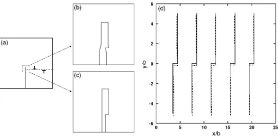
The dislocations that reach the boundary can leave the domain, producing a relative slip between the two regions in which the crystal is divided by the slip plane. This effect can be approximately included by placing the dislocation which has exited the crystal in a fictitious position along its slip plane but far away from the domain . This dislocation is not taken into account to compute the stresses in the domain but the deformation field (which is almost identical to the exact slip caused by the dislocation glide) is included to determine the total displacements of the domain. From a practical viewpoint, the fictitious dislocations are only required for the solution of problem P.
This strategy is a very accurate approximation in convex crystals but it cannot be generalized in the case of non-convex domains as it might lead to inaccurate results in particular cases. According to the idea previously described, the residual displacement associated with the dislocations which have left the domain has to be introduced by placing a fixed, fictitious dislocation on the extension of the slip plane, but far away from the boundary. This is always possible if the prolongation of the slip plane from the exit point does not cut the domain but it may not be so in non-convex domains if the prolongation of the slip plane cuts again the domain. A relevant example can be found in figure 2(a) which considers a square domain with a sharp crack. Dislocations can move in one slip plane (dashed line) which is limited by the crack and the domain external surface. Let us assume that a dislocation dipole is generated within the plane and both dislocations glide until they exit the domain. The residual displacement field due to the dislocations which have left the domain is the horizontal displacement jump of magnitude b at the slip plane while the vertical displacement is zero in the whole domain, figure 2(c). In the original approach, this field has to be reproduced by placing two fictitious dislocations far away from the domain. This can be done for the dislocation which has exited the domain through the external surface, but not for the other one, which has to be placed within the crack. The resulting displacement field due to both dislocations is shown in figure 2(b), and it is obviously different from the exact solution. These differences are plotted in figure 2(d), in which the exact (solid lines) and approximate (dashed lines) displacement fields are presented for the solutions shown in figures 2(b) and (c), respectively.
3. Modeling dislocations leaving non-convex domains
5 10 15 20 25 x/b
Figure 2. (a) Square domain with a sharp crack whose thickness is 2b. The dashed line represents a slip plane with a dislocation dipole. (b) Total displacement field around the crack tip once the dislocations have left the domain computed by placing one dislocation within the crack and the other far away from the domain, (c) Exact solution for the total displacement field around the crack tip when both dislocations have left the domain, (d) Approximate ( ) and exact ( ) displacements fields in the cracked square domain around the slip plane which is located at y = 0 for the solutions shown in (b) and (c), respectively.
a different procedure to account for the effect of dislocations leaving the crystal in convex domains. Unlike the strategy detailed in the previous section, the new method is purely numerical and works by modifying the statement of problem P. It accounts for discontinuities that exit the domain by accumulating the displacements due to plastic slip in the elements of the finite element mesh.
For simplicity of exposition, let us consider only two dislocations of a loop moving on a slip plane, as in the example of figure 2. If one of the dislocations reaches the boundary of the crystal, the resulting displacement field is similar to the sum of the displacements due to the remaining dislocation plus a discontinuous displacement field with a jump across the slip plane of value b/2. This can be approximated by adding equal and opposite displacements of magnitude b/4 above and below the slip plane, respectively. Once the second dislocation leaves the domain, and an additional displacement jump is added, this approximate solution becomes exact. We observe that placing the dislocations that have left the domain on the prolongation of the slip line far away from the boundary essentially produces the same effect as the proposed additional displacement jump, and the technique proposed in this section and the original one yield identical results.
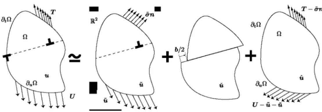
The new approach, however, has a drawback that needs to be corrected: in non-convex bodies, slip planes do not always partition the domain into two regions, one above and another below the slip plane (see, for instance, the domain in figure 2). Nevertheless, this new approach can be extended to include the effect of dislocations reaching the boundary of any two-dimensional domain. Let us consider first the analysis of a deformable crystal, free of imposed displacements and tractions on its surface, with a pair of edge dislocations of opposite sign and Burgers vector b moving on a slip plane. The crystal may be non-convex and have holes or cracks inside. When one dislocation reaches the boundary, the state in the body can be approximated by superposing the effects of a stress-free slip of magnitude b/2 across the plane and of the remaining dislocation. In physical terms, this situation can be reproduced by
(b)
e
Figure 3. Problem decomposition. The complete problem with discontinuities reaching the crystal boundaries is approximated by the sum of three simpler problems. The four problems will be referred to, from left to right, as Q, Q, Q and Q.
considering the stress field produced by the dislocation inside the body and by making a cut in the body along the slip segment, moving apart the two sides at a relative distance of b/2 and welding them back together. The process of cutting and welding is purely kinematic and no stresses would appear in the body if the two sides were free to move with respect to each other. Nevertheless, the relative slip will cause stresses in the whole domain in many cases: for example, when the domain includes holes or cracks and the slip segment extends from the surface of the hole or crack to the external boundary.
The displacement and stress fields due to the dislocation inside the domain can be computed using the methodology outlined in section 2. The slip across the plane remains to be included somehow. To mathematically describe this state of deformation, let T denote the line at the intersection of the slip plane and the plane of the domain. Ifw is the oriented normal of T and
x is a point of the domain lying on T, the jump in any scalar, vector or tensor field </> can be
expressed in terms of the jump operator [-]r defined as
[0]Jr := lim <p{x + en) - <p{x - en), (4)
where x is a point on the plane T and n is its oriented unit normal.
If u denotes the displacement field of the body, the effect of a dislocation that reaches the domain boundary T is approximated by a jump expressed as
M r = *• (5)
When both dislocations reach opposite ends of r , the effects of the slip add up as
M r = b, (6)
which is the exact solution. Of course, if both dislocations move to the same endpoint of T, their corresponding slips cancel and the jump in the displacement field disappears. The procedure described is completely general and does not require convexity of the domain.
The most general case, denoted as problem Q, consists of a deformable elastic domain with imposed displacements U on the boundary du Q, and imposed tractions T on its boundary
dtQ, dislocations moving on their corresponding slip planes and dislocations that have reached
with displacement discontinuities across the slip planes in which one or more dislocations have reached the boundary, and it is obtained by a linear combination of simpler solutions of the type schematized in figure 3. The last problem, denoted problem Q, is an elastic boundary value problem on the crystal with the displacement boundary conditions of problem Q corrected with the values obtained in problems Q and Q.
The solution to problem Q within the framework of the finite element method is described in the next section. We note that in the case of a convex body such as the one in figure 3, problem Q has a stress-free solution but affects the global stress field through its displacement M, which appears in the displacement boundary conditions of problem Q.
4. Elastic problems with displacement discontinuities
The 2D simulation of dislocation dynamics in arbitrarily shaped bodies in the presence of dislocations that exit the domain can be achieved by incorporating in the analysis the displacement jump across those slip segments on which these dislocations have glided. This can be done systematically and efficiently by embedding the discontinuities in the finite element solution, a strategy often employed in the numerical simulation of strain localization in solids. The basic ideas are borrowed from the so-called strong discontinuity approach,
, and which has been extended and applied by many others . A related approach to model dislocations based on the extended finite element method should be mentioned here
Consider problem Q, described in section 3. Its solution « is a smooth function in Q except on the segment T, in which there is a discontinuity whose value is known a priori. The displacement jump I « ]r is not due to the action of any force or stress on the body and thus the stresses are smooth across the discontinuity. The key idea for including the effect of dislocations leaving the crystal is to incorporate the plastic slip by means of displacement jumps in the finite element problem Q. In practice, this amounts to solving problems Q and Q
simultaneously.
Let uc and crc denote, respectively, the displacement and stress fields resulting from the
combination of problems Q and Q. These displacements and stresses account for the image forces that correct the solution of problem Q and capture the effect of the discontinuities.
In order to formulate the elastic problem for uc in such a way that it can be later incorporated
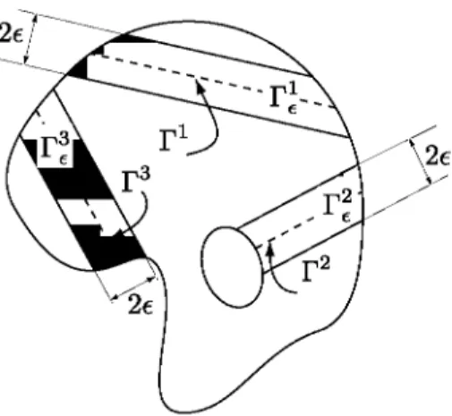
in the finite element equations some new objects need to be defined. First, let Te be the set
rc := [x e Q,, distance^, T) < e}, with the condition rc n duQ, = 0. (7)
This set is a band of width 2e around the discontinuity I\ Although it is not necessary for the derivation, it will be assumed that e is much smaller than a characteristic dimension of the body, for example, its diameter. See figure 4 for an illustration of this idea.
Let M be a known displacement function that verifies
u(x) = 0 for x i Te, [M]r = b/2, |[Vw]]r = 0. (8)
In addition, the function u must be smooth in Q\T. The strain due to u is the tensor e whose definition, away from T, is
e(x) := Vsu(x), (9)
where Vs denotes the symmetric part of the gradient. At points x not on the discontinuity, an
elastic and isotropic constitutive law defines the stress tensor by the relation
a(x) := Ce(x), (10)
Figure 4. Regions 1% in which the effect of the displacement discontinuities is localized. Three discontinuities are depicted.
The total displacement uc is the combination of the solutions to problems Q and Q and
can be written as
uc{x) := u(x) + u(x). (11)
u is a smooth function, continuous everywhere in Q. which must furthermore satisfy the
displacement boundary conditions of problem Q. The total strain at x £ V can be expressed as
Vsuc(x) = i(x) + s(x), with i(x) := Vsu(x), sc(x) := VJHC(JC) = i(x) + s(x),
and the corresponding stress tensor is given by
crc(x) := CEC(JC) = cr{x) + cr(x), with <r(x) := Cs(x).
(12)
(13)
It has been argued that the stress field in the whole crystal must be smooth. Since cr is smooth by construction, it follows from the previous equation that cr must also be smooth. The stresses at the discontinuity cannot be obtained from a constitutive equation; thus a(x) when x belongs to T has to be obtained by finding the appropriate limit of the stress tensor
a from either side of the discontinuity (which should be identical because, by construction,
[V«]|r = 0 see definition (8)).
By means of the split (11), the only unknown of the combination of problems Q and Q is the smooth displacement field u. The following boundary value problem expresses the equilibrium of the total stress crc and the boundary conditions for the total displacement uc
and tractions, but as a function of the two fields M and u
(14)
In these equations, a is a known quantity, well defined at every point of £2. The advantage of the proposed equations over the standard boundary value problem for the total displacement
uc is that the solution u of (14) is smooth and need not account for the jump across I\
-div(<x + cr) = 0
a = C e
£ = VSU
(cr + cr)n = T — crn
u = U — u — u
in Q.,
in Q.,
in Q.,
on 3f£2,
Figure 5. A finite element mesh of the crystal in figure 3. The set 1% is identified.
Moreover, the weak form of (14) can be readily obtained. Let g be a smooth function defined on Q with g =U — u — ii on duQ, and define the following function space:
V={w:£2^R2, w = 0ondu£2}. (15)
The weak solution of problem (14) is the function u such that u — g e V which verifies
f (a + a)-Vrj d^2 = f (T - an) • rjdS (16)
for all r] e V. In the previous equation, the dots stand for the inner products of the vectors or tensor on which they operate. Expression (16) is just a statement of the principle of virtual displacements for the field u with an extra term a that accounts for the effects of the discontinuity. The problem is linear; hence, the result of more than one discontinuity can be obtained by superposition of additional known stress fields similar to a.
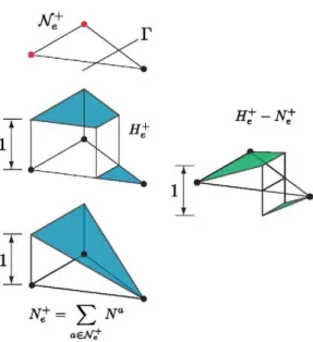
5. Finite elements with embedded displacement discontinuities
The variational formulation (16) can be discretized using the finite element method to find an approximation for the unknown part of the displacement, the function u. The total displacement in problem Q can then be recovered by using (11). The only remaining difficulty in discretizing (16) is to construct a discontinuous function ii with the properties stated in (8). This can be done easily and at an almost negligible cost.
Given a finite element mesh, the domain Q, is partitioned into «ei elements occupying a subset Q,e c £2 and connected at «node nodes of coordinates xa, a = 1,... ,«node (figure 5). Let rc be the set of all elements crossed by the discontinuity, i.e.
I \ = (J £2e. (17)
£2enr^0
The discontinuous function ii can be defined in an element-by-element fashion and is denoted uh. First, let uh be identically zero in all the elements that do not belong to Ve. The
discontinuity T splits the remaining elements into two parts Q,+e and S2~ which are, respectively,
above and below the discontinuity, with the sign provided by the normal n. The nodes of element e are denoted J\fe and can also be divided into two groups: those located above the
H+-N+
Figure 6. Discontinuity interpolation functions. The element S2e has a discontinuity at line r ,
located within the element.
Let H+(x) be the discontinuous function defined in £2e whose value is one in £2+e and zero in
Q~. The function u in element e is defined to be
^ h / \ U (X) tte
H:(X)- J ] JVa(*)|6/2, aeM*
(18)
where Na stands for the standard finite element interpolation function associated with node a.
The support of w is the band 1%, continuous everywhere except at the discontinuity T which exhibits a jump in value b/2. Its gradient is also continuous across I\ thus satisfying all the requirements put forward in (8). See figure 6 for an illustration of this idea.
The description of the finite element formulation is completed with the discretization of the trial space V which is done in the standard fashion. Given the finite element mesh, the set
Vh c V is defined as follows:
Vh \wh Y^Na(x)wa, wh = 0 on duQ\ . (19)
The finite element approximation to the displacement uc is denoted uh and,
mimicking (11), it can be split into a continuous and a discontinuous part:
u\x) :-- uh(x) + uh(x). (20)
If g is a known function that satisfies the displacement boundary conditions, the finite element approximation uh is a function such that uh — gh belongs to Vh which verifies
/ (a + a) • Vrjh d£2 = f (T - an) • rjh dS (21)
for all rjh eVh. The stress tensors are obtained as explained in section 4.
W = 4 jim
4 \tm
L= 12 jjm
Figure 7. Schematic of the geometry and boundary conditions of a rectangular single crystal with a hole subjected to uniaxial tension. There is only one slip plane with a dislocation source in the middle.
elements which intersect the discontinuity. These terms do not depend on the unknown field uh
and thus they do not modify the value of the stiffness matrix. As a result, the stiffness matrix should be computed (and factorized) only once regardless of the number of discontinuities embedded in the domain. The total displacement uh has a continuous contribution and a
discontinuous one, as indicated in (20).
It is interesting to note that the discontinuous part uh has a zero value at all the nodes of
the finite element mesh. Thus, at nodal coordinates xa, a = 1,... ,«node, ~.h,
uh(xa) :«"(*"). (22)
This property is very convenient for postprocessing the solution, making the computation of the total displacement field unnecessary. The total stress a = a + a is required, however, to compute the resolved shear stress in the dislocations (2). As explained above, the extra term due to the discontinuity has an almost negligible computational cost.
Since the nodal values of uh are zero and this field only appears in the finite element
equations (21) through its strain, it turns out that the function itself is completely unnecessary. In order to account for the effects of the slip, it suffices to compute the strain e in the elements belonging to 1%. From (18), this extra strain can be computed as
e W l o = - | * ® > ! VJVa(*) | , (23) i ae
E
aeM*
where the notation (•) indicates the symmetric part of the tensor.
6. Examples of application
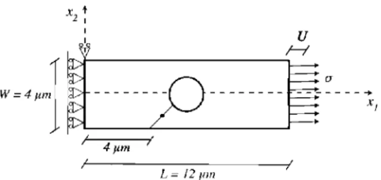
6.1. Tensile deformation of single crystal with a void
An academic application of this approach is depicted in figure 7: a rectangular single crystal of 12 /xm x 4 /xm with a circular hole of 2 /xm diameter at the center was subjected to uniaxial tension. The beam was made up of a linear elastic and isotropic solid, characterized by its shear modulus \x = 26.32 GPa and Poisson's ratio v = 0.33. Plane strain conditions are assumed in the x\-x2 plane and there was only one slip plane in the beam oriented at 45° with
e = u/L
Figure 8. The stress-strain curve of the rectangular single crystal with a hole of figure 7 subjected to uniaxial tension. The corresponding curve for the crystal without the hole is also plotted for comparison.
and the nucleation time was 0.01 /xs. Once generated, dislocations slip in the glide plane and the speed of the dislocations is given by the resolved shear stress on the glide plane and the drag coefficient B = 10~4 Pa s according to equation (1). These magnitudes are equal to those used previously in [8]. There were no obstacles to dislocation motion in the slip plane.
The boundary conditions for uniaxial tension are expressed as (figure 7)
u\ = 0 and T2 = 0 on x\ = 0,
ui = U and T2 = 0 on i , = L, (24)
7i = T2 = 0 on x2 = ±W/2,
where Ti = a^nj is the traction on the boundary with normal «,-. Loading was imposed by applying a constant strain rate of e = U/L = 2000 s_ 1. The applied stress a is computed as
1 fW/2
a = —\ T1(L,X2)dx2 (25)
W J-W/2
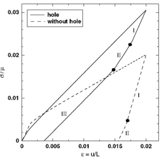
to obtain the uniaxial stress-strain curve (er//x, U/L), which is plotted in figure 8. The corresponding curve for the crystal without the hole is also plotted for comparison. In this latter situation, the slip plane extended through the whole section of the rectangular crystal, and the dislocation source was located at the center of the slip plane.
Figure 9. Residual stress distribution in the single crystal with a hole deformed in uniaxial tension after complete unloading. The Von Mises stress is shown in the plot. The displacement magnification factor is 1.
stress-strain curve upon unloading (region I in figure 8) was a compromise between the forward deformation due to dislocation motion and the backward elastic strain. This was followed by an elastic unloading (region II in figure 8) until zero stress in the crystal without the hole. The region of the elastic unloading was, however, very short in the crystal with a hole and it was followed by region III, in which the dislocation source was again activated and dislocations slip in the opposite direction. As a result of the reversed plastic flow, the permanent strain of the crystal with a hole after complete unloading was only one-fourth of the one of the crystal without a hole. The differences in behavior upon unloading between the crystals with and without a hole were due to the development of residual stresses in the crystal with a hole as a result of the inhomogeneous strain field generated by plastic slip. The magnitude of residual stresses after complete unloading of the crystal is shown in the contour plot of figure 9. The plot also shows the deformation of the crystal and the localization of the plastic strain around the slip plane. In the case of the crystal without a hole, the dislocations leaving the crystal through the edges only induced a displacement jump at both sides of the slip plane but no residual stresses.
6.2. Microvoid growth
Another example of application is the growth of a microvoid within a square single crystal grain of dimensions l x l /xm2 (figure 10). The microvoid radius R was 0.2185/xm, which corresponds to an initial void volume fraction of 15%. The crystal has two slip systems oriented at angles </> = ±35.25° with respect to the main loading axis x2. This orientation corresponds to a planar model of a FCC crystal in which the x2 direction is close to the [1 10] direction and </> stands for the angle between the x2 axis and the [1 12] orientation . The elastic constants and Burgers vector of the crystal are the same used above, and the distance between the slip planes was 81.7&. Dislocation sources were randomly distributed along the slip planes with a density of 150 /zirr2. The slip planes were initially free of dislocations. The critical resolved shear stress for dislocation nucleation was assigned randomly to the sources following a Gaussian distribution with an average value of 50MPa, a standard deviation of 15 MPa and a nucleation time of 0.01 /xs. There were no obstacles to dislocation motion within the crystal surfaces but the boundaries were assumed to act as grain boundaries impenetrable to dislocations, and so dislocations could only leave the crystal through the central void.
6~P era b~6 trq 6~P n~?i rrrt rrn frn rrn rrA frrt frn rrrt frrt frrt
F i g u r e 10. Schematic of the geometry, boundary conditions and slip systems of a square single crystal with a central hole. See text for details.
for uniaxial tension are expressed as (figure 10)
u\ = 0 and T2 = 0 on x\ = 0,
u2 = 0 and 7\ = 0 on x2 = 0, (26)
u2 = U and 7i = 0 on x2 = L,
T\ = T2 = 0 on xi = L,
while the last equation in (26) in the case of uniaxial deformation is substituted by
u\ = 0 and T2 = 0 on xi = L (27)
or by
Ml [/ and T2 = 0 on x\ (28)
for biaxial deformation. Loading was imposed by applying a constant strain rate of e =
U/L = 2000 s_ 1 up to a maximum strain of 1% under biaxial deformation and of 2% under uniaxial strain and uniaxial tension.
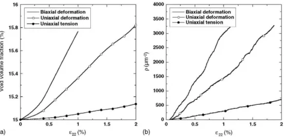
The evolution of the void volume fraction with applied strain is plotted in figure 11(a) for the three different loading cases considered. For the small deformations considered here and after the elastic region, the growth rate was practically linear in all cases, but the higher the triaxiality, the higher the void growth rate, as expected. Higher stresses facilitate the nucleation of dislocation dipoles along both slip systems, and dislocation density increased with stress triaxiality, figure 11 (b). The dislocations of each dipole moved along opposite directions driven
16
- Biaxial deformation - Uniaxial deformation - Uniaxial tension
4000
3500
3000
2500
2000
1500
1000
500
0
-Biaxial deformation —o— Uniaxial deformation — • — Uniaxial tension
/
-e22 (%) (b) £2 2( % )
Figure 11. (a) Void volume fraction as a function of the applied strain for the single crystal with a circular hole loaded in uniaxial tension, uniaxial deformation and biaxial deformation, (b) Evolution of dislocation density within the single crystal under similar conditions.
Figure 12. Dislocation pattern in the single crystal subjected to a uniaxial deformation of 2%.
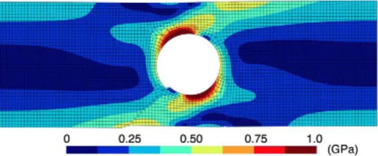
of dislocation dipoles generated under triaxial stress states increased the void growth rate. As observed in previous simulations and experiments in micrometer-sized single crystals, deformation is not homogeneous at this scale and tends to be concentrated in particular slip systems. Similar results were found in the presence of a hole and the dislocation activity was concentrated on a few slip planes, leading to the irregular shape of the void surface (figure 13) and to the formation of intense slip bands, as shown in figure 14 for the crystal subjected to uniaxial deformation.
Biaxial deformation
Uniaxial deformation Uniaxial tension
Figure 13. Influence of the stress triaxiality on the shape of the void.
0 0.25 0.50 0.75
Figure 14. Contour plot of the equivalent strain in the single crystal subjected to a uniaxial deformation of 2%, showing the inhomogeneous pattern of deformation, which is mainly localized along slip bands. The displacement magnification factor is 1.
the length scale which appears in the constitutive equations developed within the framework of strain gradient crystal plasticity. These topics will be addressed in future investigations.
7. Summary and conclusions
leaving the crystal through a free surface in the case of non-convex domains, in which the intersection of the slip plane with the domain is not a continuous segment. This particular configuration often arises in the simulation of the mechanical behavior of micro-electro-mechanical and micro-electronics devices or in micromechanics. The new method incorporates the displacement jumps across the slip segments of the dislocations that have exited the crystal within the finite element analysis carried out to compute the image stresses on the dislocations induced by the finite boundaries. This is done in a simple computationally efficient way by embedding the discontinuities in the finite element solution, a strategy often employed in the numerical simulation of crack propagation in solids. The mathematical foundations of the new approach and its practical implementation within a finite element program are detailed and two academic examples of application are presented. The first one shows the influence of the residual stresses generated by an inhomogeneous slip during forward and reversed tensile loading of a single crystal with a hole and the second one studies the growth of a void in a micrometer-sized square crystal under different levels of triaxiality.
Acknowledgments
The financial support from the Comunidad de Madrid through the program ESTRUMAT-CM and the Ministerio de Education y Ciencia de Espafia through grants DPI2006-14104 and MAT2006-2602 is gratefully acknowledged.
Appendix. Numerical implementation of embedded discontinuities
This appendix provides the details of numerical implementation to embed discontinuities within the context of the finite element method. The methodology requires one preprocessing step and modification of the standard rule for evaluating the internal force in the elements.
Preprocess. The additional stress tensors a (see (21)) to be added to the elastic stress a in
case a dislocation exits the crystal are stored in the preprocessing step. Loop over all elements e:
Loop over all slip lines d:
Let bd = bmd, where md is the oriented unit tangent vector on the line.
If the slip line d crosses element e then:
Compute (inactive) extra strain and stress, and store the stresses:
End if.
End loop over all slip lines. End loop over all elements.
Computation of internal forces. The dislocations that leave the crystal modify the calculation
of the internal forces simply by shifting the value of the stresses at the integration points. Loop over all elements e:
Compute stress due to smooth displacement cre = CVsu.
Let Xd be the (signed) number of dislocations which were on plane Td and have
left the crystal through the endpoint indicated by md.
If the slip line d crosses element e and Xd ^ 0 then Add extra stress: ae = ere + Xd <re
,d-End if.
End loop over all slip lines.
Combine stress contributions ae = ae + ae.
End loop over all elements.
The extra terms eretd do not depend on the unknown nodal variables ua, hence the modifications
due to the dislocations which have left the domain do not contribute at all to the stiffness matrix.
References
Van der Giessen E and Needleman A 1995 Modelling Simul. Mater. Sci. Eng. 3 689 Needleman A 2000 Acta Mater. 48 105
Devincre B, Kubin LP, Lemearchand C and Madec R 2001 Mater. Sci. Eng. A 309-310 211 Gates T S, Odegard G M, Frankland S J V and Clancy T C 2005 Comput. Sci. Technol. 65 2416 Gonzalez C and LLorca J 2006 Acta Mater. 54 4171
Bulatov V V and Cai W 2006 Computer Simulations of Dislocations (Oxford: Oxford University Press) Cleveringa H H M, Van der Giessen E and Needleman A 1999 Int. J. Plast. 15 837
Segurado J, LLorca J and Romero I 2007 Modelling Simul. Mater. Sci. Eng. 15 S361 Widjaja A, Van der Giessen E and Needleman A 2005 Mater. Sci. Eng. A 400^101 456
Balint D S, Deshpande V S, Needleman A and Van der Giessen E 2006 Modelling Simul. Mater. Sci. Eng. 14 409 Chng A C, O'Day M P, Curtin W A, Tay A O A and Lim K M 2006 Acta Mater. 54 1017
Deshpande V S, Needleman A and Van der Giessen E 2003 J. Mech. Phys. Solids 51 2057 Schwarz K W and Chidambarrao D 2005 Mater. Sci. Eng. A 401^101 435
Huang M, Li Z and Wang C 2007 Acta Mater. 55 1387
Lee D, Wei X, Zhao M, Chen X, Jun J C, Hone J and Kysar J W 2007 Modelling Simul. Mater. Sci. Eng. 15 S181 Biener J, Hodge A M, Hayes J R, Volkert C A, Hamza A V, Zepeda-Ruiz L A and Abraham F F 2006 Nano Lett.
6 2379
Gracie R, Ventura G and Belytschko T 2007 Int. J. Numer. Methods Eng. 69 423 Gracie R, Oswald J and Belytschko T 2008 /. Mech. Phys. Solids 56 200 Lemarchand C, Devincre B and Kubin L P 2001 /. Mech. Phys. Solids 46 1969
Deshpande V S, Needleman A and Van der Giessen E 2005 J. Mech. Phys. Solids 53 2661 Simo J C, Oliver J and Armero F 1993 Comput. Mech. 12 277
Armero F and Garikipati K 1996 Int. J. Solids Struct. 33 2863 Borja R I 2000 Comput. Methods Appl. Mech. Eng. 190 1529 Jirasek M 2000 Comput. Methods Appl. Mech. Eng. 188 307
Oliver J, Huespe A E, Pulido M D G and Chaves E 2002 Eng. Fract. Mech. 69 113
Sancho J M, Planas J, Fathy A, Galvez J and Cendon D 2006 Int. J. Numer. Anal. Meth. Geom. 31 173 Benzerga A A, Brechet Y, Needleman A and Van der Giessen E 2004 Modelling Simul. Mater. Sci. Eng. 12 159 Uchic M D, Dimiduk D M, Florando J N and Nix W D 2004 Science 305 986