Modeling and control theory applied to the wine fermentation process

(1)

UNIVERSIDAD NACIONAL DE

INGENIERIA

Facultad de Ciencias

TESIS

“MODELING AND CONTROL THEORY

APPLIED TO THE WINE

FERMENTATION PROCESS”

Para optar el grado acad´emico de Maestro en Ciencias

en Matem´

atica Aplicada

ELABORADA POR

Carlos Alberto Santana Rosas

ASESOR LOCAL

Dr. Eladio Te´

ofilo Oca˜

na Anaya (IMCA, Per´

u)

ASESORA EXTERNA

Dra. C´

eline Casenave (INRA, Francia)

(2)

To my father for being mi inspiration to never give up in difficult situations in life.

To my mother for theaching me good values and always supporting me.

(3)

Acknowledgements

To my adviser Eladio Oca˜na for trusting me, supporting me and giving me the opportunity to go to France to do the thesis in a totally different area.

(4)

(5)

Abstract

The thesis has two purposes: The first one is to build a mathematical model that better approximates (with respect to the mathematical model in [2]) to the behaviour of the wine fermentation process with the addition of certain amount of nitrogen at some instant of time, based in [2]. This mathematical model is described by mean ordinary differential equations including some parameters which will be identified solving some optimization problems.

(8)

(9)

Introduction

One of the most important steps in the wine production is the fermentation process. The fermentation process consists in the bioconversion of glucose into ethanol and other metabolites which give to the wine a part of its organoleptic characteristics (glycerol, organic acid, aromatic compounds, etc). The yeasts are the ones who perform this con-version. The metabolism of yeast is very complex and it a reason that is continuously studied. Aforetime, the wine fermentation was done manually and empirically. Currently, it is automated in big tanks to do wines to big scales, minimizing the time and the energy consumption, this is the major challenges for oenologists. To do that, first we must study the behaviour of the wine fermentation, this behaviour is represented through a mathe-matical model, in this case are ordinary differential equations. Then, we must control the dynamical system such that the output of the system stabilizes at a desired value (called setpoint), to do that we are going to use the tools of control theory.

The nitrogen addition during the wine fermentation is a oenological condition, that is to say, the oenologists use that in the wine production to accelerate the fermentation. Before 2004, researchers try to do mathematical models with this oenological condition but unfortunately they are poorly adapted. In 2004, Malherbe made a mathematical model with this oenological condition [2] where that works well in some experiments but others do not. So, one of the two main purpose of this thesis is to improve this mathematical model. The experiments for the creation of the mathematical model are realized in a batch reactor [1], it is a closed tank where there are chemical concentrations (yeast, nitrogen, glucose transporter, glucose, ethanol).

Then, this model is transformed in a mathematical model with control (state-space representation) in a tank like the batch reactor but the difference is that it is added concentrations of nitrogen, glucose transporter, glucose and ethanol with certain velocities

Q1,Q2 and it is removed concentrations of nitrogen, yeast, glucose transporter, sugar and

ethanol with certain velocity Q = Q1 +Q2. The velocities Q1 and Q2 are the controls

or input. This kind of tank is called continuous stirred tank bioreactor. The other main purpose of this thesis is to control or manipulate the wine fermentation, that is to say, we are going to add and remove concentration in the continuous bioreactor with certain velocities Q1 and Q2 such that the sugar S and the rate production V CO2 stabilizes at

the desired valuesS∗ and V CO∗₂ respectively. To do that, we are going to use the tools of control theory for MIMO non linear system [6].

(10)

and biological behaviour of the wine fermentation process with the addition of nitrogen at certain instant of time. Also, we will do the simulation of the mathematical model and then compare it with the experimental data of certain chemical concentrations of the wine fermentation.

The main purpose of Chapter 2 is to build a mathematical model to obtain a better approximation (with respect to the mathematical model in Chapter 1) to the behaviour of the wine fermentation process. This construction is constituted by certain parameters that will be identified solving numerically step by step some optimization problems in python language.

The main purpose of Chapter 3 is to study the mathematical model of Chapter 2 but adding control variables. It is made in a tank like the batch reactor but the difference is that it is added concentrations of N, S, E with certain velocity Q1, Q2 and is removed

concentrations of N, X, T r, S, E with certain velocityQ. We are going to assume that the input rate is equal to the output rate (Q1+Q2 =Q), that is to say the volume is constant

because dV_dt = Q−(Q1 +Q2). A tank with this assumption is called continuous stirred

tank bioreactor.

Assuming that a MIMO linear system control problem without constraint is solved, that is to say, it is finded a inputuwc _{such that the output}_ywc_{stabilizes in a some sense at}

a known desirable constant value y∗. So, the main purpose of Chapter 4 is to find a input ˜

u of the same linear system control problem with constraint (the input ˜u is restricted) such that the output y is close to ywc _{as much as possible at each instant of time. This}

was done in the article [4] and we are going to do that with more details and give the implicit solution of an example.

The main purpose of Chapter 5 is to find the input ˜u of a single-input single output (SISO) nonlinear system control problem with constraints such that the outputystabilizes at a known desirable constant value y∗ and is to close to ywc as possible at each instant of time. This will be solved by linearizing the SISO system in a linear system and finally we will apply the anti-windup technique to this linear system studied in the previous chapter. This was done in the article [5] and we are going to do that with more details and give the implicit solution of an example.

The main purpose of Chapter 6 is to find the input ˜u of a multi-input multi-output (MIMO) nonlinear system control problem with constraints such that the output y is to close toywc _{at each instant of time. The solution of this control problem is a generalization}

of the case SISO nonlinear system control problem with constraints. It was done in the article [6] and we are going to do that with more details and give the implicit solution of an example.

The main purpose of Chapter 7 is to control the wine fermentation with oenological condition represented for the mathematical model presented in Chapter 3, that is to say, we are going to add and remove the chemical concentrations of the continuous bioreactor with certain velocities Q1 and Q2 such that the sugar S and the rate production V CO2

(11)

Chapter 1 Simulation of Malherbe model

1.1 Description of the Malherbe model

One of the most important steps of the wine production is the fermentation. The fermen-tation process has a difficult behaviour because of that is continuously studied to obtain a better mathematical model such that is approximated to the behaviour of the wine fermen-tation. The consequences of that are the minimization of the wine fermentation duration and the energy used in a cold tank or several tanks, it is realized by identification and automatic control tools by means of on-line monitoring of the fermentation process.

Yeast metabolism is very complex because of that the researchers try to make a math-ematical model with specific conditions necessary for the fermentation control but unfor-tunately, most of the models are poorly adapted to enological conditions.

Generally, the Assimilable Nitrogen is not taken into account at all and the temperature effects are generally unsatisfactory, but these two variables are very important because their manipulations in experiments enable to control the reactions.

1.1.1 Problem

The aim is to make a mathematical model using the recent advances in physiological knowledge (principally the effect of nitrogen) where the rate production CO2 is related

to the effects of the main factors in wine-making conditions: nitrogen additions (which must not exceed the maximal authorized level) and temperature (which can vary within a predefined range).

1.1.2 Modeling

The main component to be measured in quantity is the CO2 concentration or the rate

production dCO2/dt. In this model is measured the temperature in the tank and the

(12)

We present the dynamical model of the wine fermentation, with temperature and added ammoniacal nitrogen as the input variables and rate of CO2 production as the

output variable.

dS

dt = −2.17X(t)νST[S(t), E(t), T]NST[Nmax(t)−N(t), X(t), T] dN

dt = −X(t)νN[N(t), E(t), T] dX

dt = k1(T)X(t)

1− X(t)

Xmax(Ninit)

S(0) = Sinit

N(0) = Ninit

X(0) = Xinit

(1.1)

where t ≥ 0; X(t) yeast concentration is the cell population in the tank (cell/l); the maximum yeast concentration in a process with initial nitrogen concentration Nini is

denoted by Xmax(Ninit) (function depending of Ninit); S(t) is the glucose concentration in

the tank (g/l);E(t) is the ethanol concentration in the tank (g/l);Nmax(t) = Ninit+Nadd(t)

where Nadd is the amount of nitrogen added in the tank; T(t) temperature in the tank

(◦C) and k1(T) is the growth rate of the population in the exponential growth phase.

The functions νST, NST and νN are described in what follows. The concentrations of

glucose and ethanol are deduced directly from the amount of CO2 released. Assuming

Gay-Lussac’s law, we obtain the following equations:

S(t) = S(0)−2.17CO2(t) CO2(0) = 0

E(t) = 0.464[S(0)−S(t)] (1.2)

The yield coefficients (2.17 and 0.464) in the equation (1.2) are obtained by the work done in the paper [3].

1.1.3 Yeast activity

Yeast activity is implicitly described by four subsystems: glucose transport, glycolysis, nitrogen transport and synthesis of glucose transporters.

Glucose Transport

The function νST describes the activity of a glucose transporter with ethanol inhibition,

where the glucose enters in the membrane then by means of the glycolysis it is transformed in ethanol and CO2 release.

νST(S, E, T) =

k2(T)S

S+KS+KSISEαS

(1.3)

where KS, KSI and αS are constants, and k2 is the rate fermentation depending of

(13)

Glycolysis

Glycolytic enzymes have a high level of activity and are not inhibited by ethanol, it goes out of the membrane to obtain ethanol and_CO2 release.

Process of Nitrogen Assimilation

The function νN is related to the nitrogen absorption by the yeast which is strongly

inhibited by ethanol.

νN(N, E, T) =

k3(T)N

N +KN +KN IN EαN

(1.4)

where KN, KN I and αN are constants, and k3 is the rate fermentation depending of

temperature.

Synthesis of Glucose Transporters

The functions NST[Nmax(t), N(t), X(t), Tucd] represents the mean number of transporters

in a yeast. In this process, the cell transforms a fraction of the absorbed nitrogen into proteins that will permit the glucose transport. This relationship implies thatNST depends

on the nitrogen assimilated by a single cell and environmental conditions.

1.2 Simulation of the Malherbe model

In this section, we will present the simulation of the dynamical system (1.1) using the following parameters identified by Malherbe and the initial conditions.

1.2.1 Parameters with temperature constant

k1(T) = 0.0287T −0.3762

Xmax(Ninit) = 109(−649Ninit2 + 698Ninit+ 7)

k2(T) = exp _T_+273.15−K2

where K2 = 7000

KS = 15 KSI = 0.012 αS = 1.25

k3 = 10−12 KN = 0.03 KN I = 0.035 αN = 1.5

NST[Nmax(t)−N(t), X(t), T]×k2(T) = λaN_X(t)i(t) +λbT +λcN_X(t)i(t)T +λd

whereNi =Ninit+λ0(Nadd)[Nadd(t)−N(t)]

λ0 = 3.2 when the nitrogen addition is 0.063 g/l and λ0 = 0 without nitrogen addition.

λa= 335×109 λb = 0.061 λc= 3×109 λd =−1.

1.2.2 Initial conditions

Sinit = 200.0 g/l

(14)

1.2.3 Simulation to 24

◦

C

We present the simulation of Malherbe model using the parameters and initial conditions in the previous subsections.

Figure 1.1: Simulation of a fermentation with Ninit = 0.17 g/l.

Yeasts reproduce themselves because they have a logistic behaviour and as they grow fast, the nitrogen is consumed quickly. The sugar is consumed to produce ethanol and car-bon dioxide. The rate production increases until 25h approximately and then it decreases because the sugar is concave from 0 to 25h and then it is convex.

1.3 Comparison of the Malherbe model and the

ex-perimental data

In this section, we will compare the approach of the simulation of Malherbe model with the experimental data for the rate production and the yeast.

1.3.1 Data of the rate production

(15)

Figure 1.2: Data of the rate production (dCO2/dt).

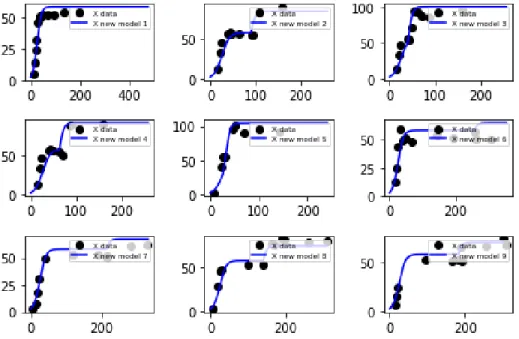
We present the approach of the simulation of Malherbe model with the experimental data for fifteen experiments:

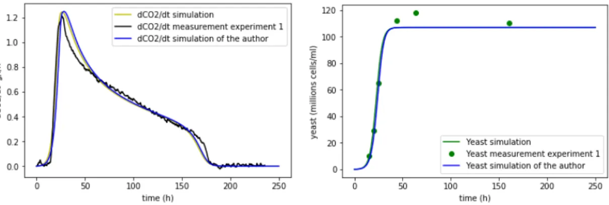
Figure 1.3: Rate production and yeast simulation of the first experiment withNinit = 0.17

g/l without nitrogen addition.

Figure 1.4: Rate production and yeast simulation of the second experiment with Ninit =

(16)

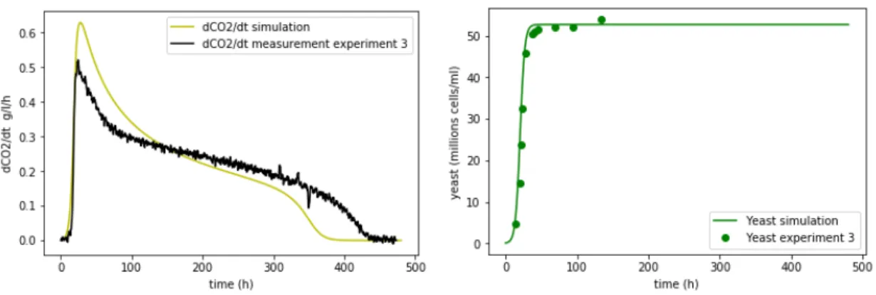
Figure 1.5: Rate production and yeast simulation of the third experiment withNinit = 0.07

g/l without nitrogen addition.

Figure 1.6: Rate production and yeast simulation of the fourth experiment with Ninit =

0.17 g/l and Nadd= 0.063 g/l at the instant t= 89.53 h.

Figure 1.7: Rate production and yeast simulation of the fifth experiment withNinit = 0.17

(17)

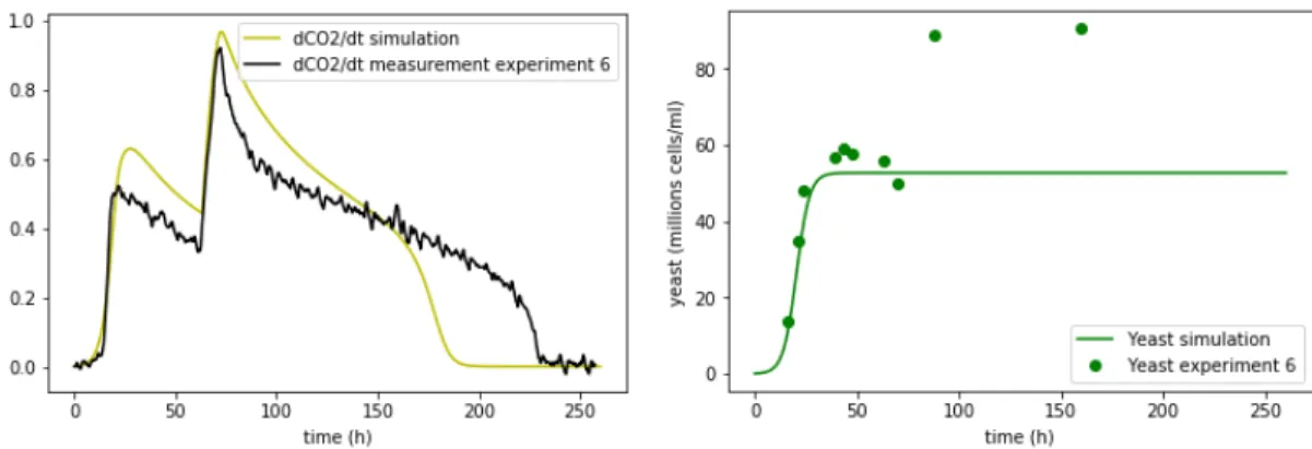
Figure 1.8: Rate production and yeast simulation of the sixth experiment withNinit = 0.17

g/l andNadd = 0.063 g/l at the instant t = 63.11 h.

Figure 1.9: Rate production and yeast simulation of the seventh experiment withNinit =

0.17 g/l and Nadd = 0.063 g/l at the instant t = 26.3 h.

Figure 1.10: Rate production and yeast simulation of the eighth experiment withNinit =

(18)

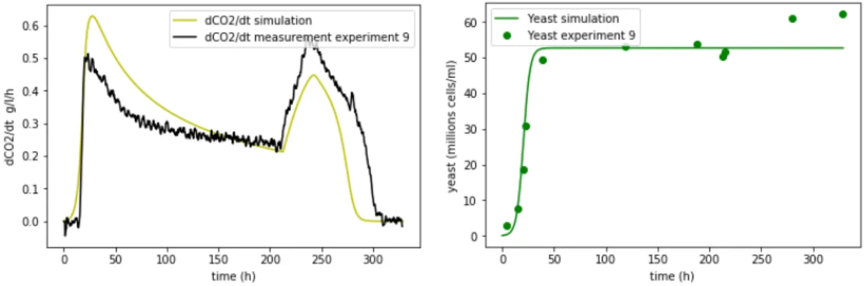
Figure 1.11: Rate production and yeast simulation of the nineth experiment with Ninit =

Figure 1.12: Rate production and yeast simulation of the tenth experiment with Ninit =

Figure 1.13: Rate production and yeast simulation of the eleventh experiment withNinit =

(19)

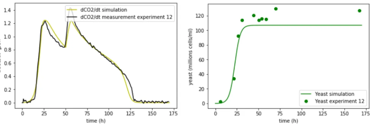
Figure 1.14: Rate production and yeast simulation of the twelfth experiment withNinit =

0.17 g/l and Nadd = 0.063 g/l at the instant t = 50.31 h.

Figure 1.15: Rate production and yeast simulation of the thirteenth experiment with

Ninit= 0.17 g/l andNadd = 0.063 g/l at the instant t= 22.81 h.

Figure 1.16: Rate production and yeast simulation of the fourteenth experiment with

(20)

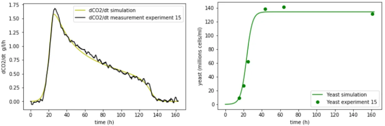
Figure 1.17: Rate production and yeast simulation of the fifteenth experiment withNinit =

0.17 g/l and Nadd= 0.063 g/l at the instant t= 0 h.

In the experiments 1 and 2, the simulation of the rate production and yeast approximate very well to the experimental datas, but in the followings experiments they do not work well. The rate production does not work well in its maximum value and in the final part of time, and yeast does not work well when there is nitrogen addition.

1.4 Comments about the quality of the model

There are some experiments where the model does not fit very well.

The dynamic equation (1.1) of the yeast only depends on the yeast and has a logistic behaviour, because of that, yeast does not reproduce. We prove that mathematically, analyzing the equilibrium points:

−XνSTNST = 0 (1.5)

−XνN = 0 (1.6)

k1[T]X[1−

X Xmax(Ninit)

] = 0 (1.7)

Biologically, we are interesed when X 6= 0. Then from equations (1.6) and (1.7), we have respectively νN = 0 and X = Xmax(Ninit). Therefore the equilibrium

(21)

x= [S, N, X]T_, _f _{= [}_f

1, f2, f3],

f1 = −XνSTNST

f2 = −XνN

f3 = k1[T]X[1− _X_maxX_(N

init)]

∂f1

∂S = −

XK2(T)KSNST

(S+KS+KSISEαS)2

<0

∂f2

∂S = 0 ∂f2

∂N = −

Xk3[T]KN

(N +KN +KN IN EalphaN)2

<0

∂f3

∂S = 0 ∂f3

∂N = 0 ∂f3

∂X = k1[T][Xmax(Ninit)−

1

Xmax(Ninit)

]

∂f

∂x(xeq) =

      ∂f1 ∂S ∂f1 ∂N ∂f1 ∂X

0 ∂f2

∂N

∂f2

∂X

0 0 −k1[T]

     

The eigenvalues in the equilibrium point xeq are ∂f_∂S1, _∂N∂f2 and −k1[T] negatives.

Therefore, the equilibrium point is stable. So that when there is not nitrogen ad-dition, the Yeast will be constant igual to Xeq = Xmax(Ninit) and when we add

nitrogen, the yeast will continue being igual Xmax(Ninit) because only depends of

the Ninit. Therefore when we add nitrogen, the yeast does not increase and does not

(22)

(23)

Chapter 2 Improvement of Malherbe model

The purpose of this chapter is to improve the Malherbe model studied in Chapter 1. This improvement leads us to consider a new model which is made step by step where there are parameters that will be identified. The parameter identifications are obtained by solving an optimization problem that will be solved numerically using python language.

2.1 Description of the new model

In this section we present the mathematical model and the biological and chemical be-haviour of the new model. In fact, the mentioned new model can be set as:

dX

dt = µ(N)Xf(S) dN

dt = −µ(N)X dS

dt = −2.17X(t)νSTT r dT r

dt = c1µ(N)X[c2−f(S)] +g(E)T r

[X(0), N(0), S(0), T r(0)] = [Xinit, Ninit, Sinit, T rinit]

whereX(t) (yeast concentration) is the cell population in the tank (cell/l);N(t) and S(t) are respectively the nitrogen and sugar concentration (g/l); andT r(t) (glucose transporter) is the number of sugar transporters in a cell. On the other hand, µ(N), f(S) and g(E) are defined as:

µ(N) : = µmaxN

kn+N

f(S) : = aS2₊_bS₊_c

g(E) : = lE2₊_mE ₊_n.

(2.1)

(24)

It is well know that the most important chemical reactions produced in the wine fermentation process are:

N −X→X+T r Growth of X (2.2)

S −−−→X,T r E+CO2 Degradation of S in ethanol (2.3)

So, by taking into account the Gay-Lussac’s law of the chemical reaction (2.3), we get the following equations:

S(t) = S(0)−2.17CO2(t) CO2(0) = 0

E(t) = 0.464[S(0)−S(t)]

where the yield coefficients (2.17 and 0.464) in the system are obtained by mean of exper-iment results as studied in [3].

In (2.2), the nitrogen is consumed to produce yeast and glucose transporter in a yeast. The proportion 1₂f(S) of nitrogen rate is used by the yeast for its growth and the comple-ment proportion (1−1

2f(S)) of nitrogen rate is used by the yeast for the synthesis of glucose

transporter. The sugar is respectively absorbed and inhibited by the yeast and ethanol, this activity is described by νST studied in Subsection 1.1.3, then the glucose transporter

permits that the sugar enters with greater velocity in the yeast. When g(E)<0, there is inhibition or degradation and when g(E)>0, there is regeneration of transporter by the yeast to adapt to the environment.

2.2 Parameter identifications of the model

In this section, we describe a method to identify the parameters involving in the mathe-matical model proposed in Section 2.1. This method consists in minimizing a quadratic error of estimation.

2.2.1 Parameter identifications of

µ

(

N

)

and

f

(

S

)

In this part, we are going to identify the parameters kn, µmax, xinit, a, b and c of the

following dynamical system using two experimental data: the nitrogen data and the yeast data.

dN

dt = −µ(N)X dX

dt = µ(N)Xf(S) N(0) = Ninit

X(0) = Xinit

where

µ(N) : = µmaxN

kn+N

f(S) : = aS2₊_bS₊_c

(25)

Method to identify the parameters

We use the traditional weighted least squares method to identify the parameterskn,µmax,

xinit, a, b and c. The idea is to minimize the following quadratic error of estimation:

min

(kn,µmax,Xinit,a,b,c)

w1||N data−N sim||22+w2||Xdata−Xsim||22

s.t.

dN

dt = −µ(N)X dX

dt = µ(N)Xf(S) N(0) = Ninit

X(0) = Xinit

                         (2.5)

where w1 and w2 are the weights (fixed positive numbers), and

N data := [(N data)1,· · · ,(N data)n]

N sim := [N(t1),· · · , N(tn)]

Xdata := [(Xdata)1,· · · ,(Xdata)m]

Xsim := [X(t1),· · · , X(tm)]

where (N data)i and (Xdata)i are respectively the data of nitrogen and yeast at time ti.

So for instance, usingN dataandXdatavectors borrowed from [2],w1 = 0.01,w2 = 10,

n= 9 andm = 12, the numerical result (using Python language) of problem (2.5) is:

        Xinit kn µmax a b c         =         3

0.35620067289411805 0.00074179295965841698

0.015807664957978633 9.3168038110079628e−07

212.34153088786363

        . (2.6)

Simulation results for yeast and nitrogen experiments

(26)

Figure 2.1: Identification of µ(N) and f(S).

2.2.2 Paremeter identifications of

f

(

S

)

Similar to the previous analysis we use the following quadratic optimization problem in order to identify the parameters a, b and cfrom f(S) using the yeast data.

min

(a,b,c) r

X

k=1

||Xdatak−Xsimk||22

s.t.

dXk

dt = µ(Nk)Xkf(Sk) dNk

dt = −µ(Nk)Xk Xk(0) = Xkinit

Nk(0) = Nkinit

                             (2.7)

where for k = 1,· · · , r, the functions µ(Nk) and f(Sk) are defined in (2.1), and

Xdatak := [(Xdatak)1,· · · ,(Xdatak)mk];

Xsimk := [Xk(t1),· · · , Xk(tmk)].

Here (Xdatak)i is the data of yeast at time ti of the kth experiment.

So for instance, by considering r = 9, m1 = m3 = m7 = m9 = 12; m2 = m4 = 10;

m5 = 8 andm6 =m8 = 12, as studied in [2] and also by takingXdatakfrom this reference,

the numerical solution of (2.7) is:

  a b c  =  

2.01142324e−02 7.53592364e−07 5.10588530e+ 01

 .

(27)

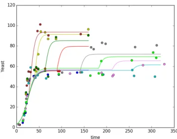
Simulation results for the yeast experiments

The following graphic describes the approach of the yeast simulation with yeast data of nine experiments each identified with different color.

Figure 2.2: Identification of f(S) using yeast data of all the experiments.

2.2.3 Parameter identifications of Glucose Transporter

Similar to the previous subsection, we will identify the paremeters c1, c2, l, m, and n of

the following dynamical system using the glucose transporter data.

dT r

dt = c1µ(N)X[c2−f(S)] +g(E)T r dX

dt = µ(N)Xf(S) dN

dt = −µ(N)X T r(0) = T rinit

X(0) = Xinit

N(0) = Ninit

where

g(E) := lE2 ₊_mE ₊_n.

Method to identify the parameters

Similar to the previous subsection, we identify the parameters c1, c2, l, m, and n using

(28)

min

(c1,c2l,m,n)

r

X

k=1

||T rdatak−T rsimk||22

s.t.

dT rk

dt = c1µ(Nk)Xk[c2−f(Sk)] +g(Ek)T rk dXk

dt = µ(Nk)Xkf(Sk) dNk

dt = −µ(Nk)Xk T rk(0) = T rkinit

Xk(0) = Xkinit

Nk(0) = Nkinit

                                             (2.8) where

T rdatak := [(T rdatak)1,· · · ,(T rdatak)mk]

T rsimk := [T rk(t1),· · ·, T rk(tmk)]

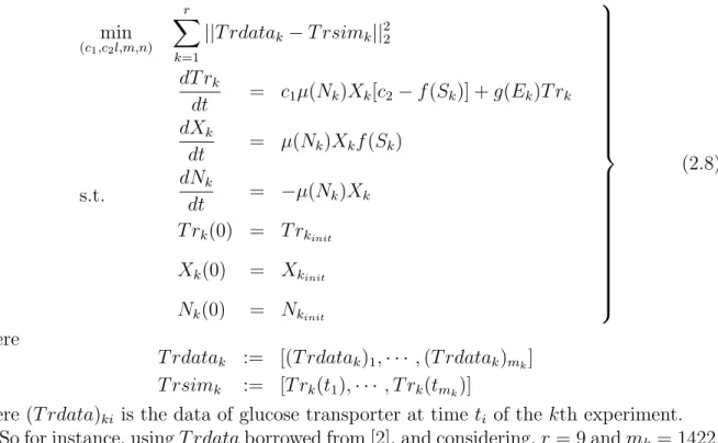
where (T rdata)ki is the data of glucose transporter at time ti of the kth experiment.

So for instance, usingT rdataborrowed from [2], and considering,r = 9 andmk = 1422,

the numerical solution of problem (2.8) is:

      c1 c2 l m n       =      

2.99621981e−02 1.44460425e+ 03

−1.31367315e−06 1.50119898e−04

−3.06341075e−03

      .

Simulation results of glucose transporter experiments

The following graphic describes the approach of the glucose transporter with the glucose tranporter data of nine experiments.

(29)

2.3 Simulation of the new mathematical model

In this section, we present the simulation of the mathematical model presented in the Section 2.1 to compare with the experimental data.

Figure 2.4: Comparison between the rate production simulation and the rate production data.

(30)

2.3.1 Comparing the two mathematical models together the

ex-perimental data

We present here the simulation results obtained from the mathematical model presented in the Section 2.1 and the malherbe model described in equation (1.1), and we compare they together with the experimental data.

Figure 2.6: Comparison between the rate production simulation of the new model, rate production simulation of the Malherbe model and the rate production data.

(31)

Chapter 3 Continuous stirred tank bioreactor

for the new mathematical model

In Chapter 2 we made a mathematical model to study the wine fermentation process with oenological conditions (nitrogen addition), the experiments are made in a batch reactor where there are concentrations in the tank. The main purpose of this chapter is to study this mathematical model but adding control variables. It is made in a tank like the batch reactor but the difference is that it is added concentrations ofN, S, Ewith certain velocity

Q1, Q2 and is removed concentrations of N, X, T r, S, E with certain velocity Q. We are

going to assume that the input rate is equal to the output rate (Q1+Q2 =Q), that is to

say the volume is constant because dV_dt =Q−(Q1 +Q2). A tank with this assumption is

called continuous stirred tank bioreactor.

3.1 Mass balance

In this section, we use the mass balance law to the chemical concentrations involving in the dynamical system of the Section 2.1. Therefore, the dynamical behaviour of the nitrogen is equal to−µ(N)XV which is the rate of nitrogen comsuption in the tank; NinQ1+NaddQ2

is the nitrogen rate that come into the tank with different dilution rate Q1 and Q2; and

finally −N Qis the nitrogen rate leaving the tank. The dynamical behaviour of the other concentrations have the same structure.

d(N V)

dt = −µ(N)XV +NinQ1+NaddQ2−N Q d(XV)

dt = µ(N)f(S)XV −XQ d(T rV)

dt = [c1µ(N)X(c2−f(S)) +g(E)T r]V −T rQ d(SV)

dt = −ν(E, S)T rV +SinQ1−SQ d(EV)

dt = 0.464ν(E, S)T rV +EinQ1−EQ

(32)

Using the dynamical system of (3.1) and the assumption of constant volumen of the tank, we obtain the mathematical model with control variables as follows:

dN

dt = −µ(N)X+ (Nin−N) Q1

V + (Nadd−N) Q2

V dX

dt = µ(N)f(S)X−X Q1

V −X Q2

V dT r

dt = c1µ(N)X(c2−f(S)) +g(E)T r−T r Q1

V −T r Q2

V dS

dt = −ν(E, S)T r+ (Sin−S) Q1

V −S Q2

V dE

dt = 0.464ν(E, S)T r+ (Ein−E) Q1

V −E Q2 V                                (3.2)

3.2 State - space representation of the wine

fermen-tation with enological condition

The mathematical model described in (3.2) can be represented by a state - space repre-sentation as follows:

dξ

dt = f(ξ) +g(ξ)u y = h(ξ)

Qmin

1 ≤u1 ≤ Qmax1

Qmin

2 ≤u2 ≤ Qmax2

             (3.3) where

ξ := [N, X, T r, S, E]t

f(ξ) :=

   

−µ(N)X µ(N)f(S)X

c1µ(N)X(c2−f(S)) +g(E)T r

0.464ν(E, S)T r

   

g(ξ) := 1

V      

Nin−N Nadd−N

−X −X

−T r −T r Sin−S −S

Ein−E −E

     

u := [u1, u2]t = [Q1, Q2]t

V CO2 := _2.171 ν(E, S)T r

(33)

Chapter 4 Anti-windup for Internal Model

Control

Assuming that a MIMO linear system control problem without constraint is solved, that is to say, it is finded a input uwc _{such that the output} _ywc _{reaches and stabilizes at a}

known desirable constant value y∗. The main purpose of this chapter is to find a input ˜u

of the same linear system control problem with constraint (the input ˜u is restricted) such that the outputy is close toywc _{as possible at each instant of time. This was done in the}

article [4] and we are going to do that with more details and give the implicit solution of an example.

4.1 Introduction

Definici´on 4.1. Let f be a real-valued, locally integrable function defined on the positive real numbers. Then

F(s) = [L(f)](s) :=

Z ∞

0

f(t)e−stdt, f =L−1[F]

denote, as usual, the direct and inverse Laplace transforms.

The scheme in Figure 4.1 is called open loop whereuenters to the system P obtaining a response y, u(t) := [u1(t), ..., un(t)]T ∈ Rn and y(t) := [y1(t), ..., yn(t)]T ∈ Rn are the

input and the output respectively.

P

Linear plant

y

u

Figure 4.1: Linear system with inputu and output y.

The elements of P(s) ∈ _Rn×n _{are quotient of polynomials and mathematically, the}

scheme of Figure 4.1 is the following

(34)

where

Y(s) = L{y(t)}:= [Y1(s), ..., Yn(s)]T ∈Rn Yi(s) = L{yi(t)}

and

U(s) = L{u(t)}:= [U1(s), ..., Un(s)]T ∈Rn Ui(s) = L{ui(t)}

are respectively the Laplace transforms of the output y and the input u. P(s) = [Pij(s)]

is called transfer function.

Remark. The equation (4.1) or the scheme of Figure 4.1 is equivalent to a system of linear ordinary differential equations.

Definici´on 4.2. A strictly proper transfer function is a transfer function where the degree of the numerator is less than the degree of the denominator. A proper transfer function is a transfer function where the degree of the numerator is less or equal to the degree of the denominator. A biproper transfer function is a transfer function where the degree of the numerator is equal to the degree of the denominator.

We define the matrixp(t) := [pij(t)]∈ Rn×n whose ij−element pij(t) = L−1[Pij(s)] is

the inverse Laplace transform of Pij.

Definici´on 4.3 (The convolution transform). The convolution transform ofp and u, denoted by p∗u, is defined on all _R as

(p∗u)(t) :=

Z t

0

p(t−τ)u(τ)dτ (4.2)

We are going to prove that the inverse Laplace transform of the product of two Laplace transforms in (4.1) is equal to the convolution transform of the two inverse Laplace trans-forms.

From equation (4.1), we have the following:

Yi(s) = n

X

j=1

Pij(s)Uj(s)

yi(t) = n

X

j=1

(pij∗uj)(t) = n

X

j=1

Z t

0

pij(t−τ)uj(τ)dτ

yi(t) =

Z t

0 n

X

j=1

pij(t−τ)uj(τ)dτ

y(t) =

Z t 0

(35)

where

vt(τ) :=

         n X j=1

p1j(t−τ)uj(τ)

.. .

n

X

j=1

pnj(t−τ)uj(τ)

        

From equation (4.2), we have that

y(t) =

Z t

0

p(t−τ)u(τ)dτ y(t) = (p∗u)(t)

4.2 Problem formulation

Foru∈_Rn_, _sat₍_u_{) := [}_sat₍_u

1), ..., u(n)]T where

sat(ui) =

    

umax_i ui > umaxi

ui umini ≤ui ≤umaxi

umin_i ui < umini

We assume that the MIMO linear system without constraint,

˙

x = Ax(t) +Bu(t)

y(t) = Cx(t)

(4.3)

whereA, B and C are given n×n real matrices withB and C invertible, is solved. Therefore, the close loop scheme

P

Linear plant

K

Controller

y

wc

y

∗

u

wc

-+

Figure 4.2: Closed loop of a linear system without constraints.

is the solution of the linear system (4.3). Whereuwc _and_ywc _{are respectively the input}

and output.

From Figure 4.2, we have the following equations:

Ywc ₌ _{P U}wc

(36)

where Ywc_, _Uwc _and _Ywc _{are respectively the Laplace transforms of} _ywc_, _uwc _and _y∗_.

From equation (4.4),

Ywc =P(I +KP)−1KY∗

LetF ∈_Rn×n _{be the Laplace transform of a function}_f_{. Therefore, using the previous}

equation

(f ∗ywc)(t) = L−1_[_{F P}₍_I₊_KP₎−1_Ky∗

](t)

The main purpose of this Chapter is to solve the MIMO linear system with constraint

˙

x = Ax(t) +Bu(t)

y(t) = Cx(t)

umin _≤_u₍_t₎_≤ _umax

  

(4.5)

or equivalent to

˙

x = Ax(t) +Bu˜(t)

y(t) = Cx(t) ˜

u(t) := sat(u(t))

   (4.6)

P

Linear plant

y

˜

u

Figure 4.3: Linear system with constraint.

such thaty is close to ywc _{as possible at each time} _t_{, that is to say, mathematically we}

want to solve the following optimization problem at each time t,

min

˜

u ||(f∗ywc)(t)−(f∗y)(t)||1= minu˜ ||L

−1_[_{F P}₍_I₊_KP₎−1_Ky∗_](_t₎₋₍_L−1_[_{F P}_]_∗_u_˜₎₍_t₎_||_1, _(4.7)

where f is a diagonal filter such that F P is biproper.

In general the IMC scheme in Figure 4.4 solves (4.6) but does not solve the optimization problem (4.7), because of that we are going to present in the next section a close loop scheme satisfying certain conditions to resolve the problems (4.6) and (4.7).

P

Linear plant

sat

()

Constraint

K

Controller

y

∗

u

˜

-+

(37)

4.3 Anti-windup design

In this section we are going to present a close loop scheme satisfying certain conditions to solve the problems (4.6) and (4.7).

Definici´on 4.4 (Stability and minimum-phase). A linear system is stable when all poles (roots of the denominator) of the elements of its transfer function have their negative real part. A linear system is minimum-phase when all zeros (roots of the numerator) of the elements of its transfer function have their negative real part.

The following Lemma is proved in the article [4].

Lemma. The following close loop

system

sat()

K1

Controller

y y∗

K2

Controller ˜

u u

+

-+

-Figure 4.5: Anti-windup linear IMC scheme.

with:

K1 :=F P(I+KP)−1K and K2 :=F P −I−K1P, and the following assumptions:

1) (I+KP)−1_K _{is biproprer, stable and minimum-phase,}

2) F P|s=∞ is a diagonal nonsingular matrix with finite elements,

3) K1 is stable and minimum-phase, 4) K1P +K2 is strictly proper,

solve (4.6) and the optimization problem (4.7).

4.4 Example

In this section, we are going to present a example and will show the perfomance of the Anti-windp method. We consider the following linear system,

˙

y = −0.01y+ 0.02u y(0) = 0

(38)

Then, the linear plant is the following:

P(s) = 2 100s+ 1. The IMC controller designed is

K = 100s+ 1 40s .

Case 1. Chossing f(s) = 2.5(20s+ 1) gives

K1 = 2.5

K2 =

−1 100s+ 1 Case 2. Chossing f(s) = 50(s+ 1) gives

K1 =

50(s+ 1) 20s+ 1

K2 =

18802−1 (100s+ 1)(20s+ 1)

4.4.1 Close loop

a) Unconstrain system is obtained by the scheme in Figure 4.2:

Y = P U

U = K(Y∗−Y) The mathematical equations are the following:

˙

y = −0.01y+ 0.02u u = 2.5(y∗−y) +z

where

˙

z = 0.025(y∗−y) [y(0), z(0)] = [0,0]

b) IMC system is obtained by the scheme in Figure 4.4:

Y = PU˜

˜

u = sat(u)

U = K(Y∗−Y) The mathematical equations are the following:

˙

y = −0.01y+ 0.02˜u

˜

u = sat(u)

u = 2.5(y∗−y) +z

where

˙

(39)

c) Anti-windup IMC case 1 is obtained by the scheme in Figure 4.5:

Y = PU˜

˜

u = sat(u)

U = K1(Y∗−Y)−K2U˜

The mathematical equations are the following:

˙

y = −0.01y+ 0.02˜u

˜

u = sat(u)

u = 2.5(y∗−y) +z

where

˙

z = 0.01(−z+ ˜u) [y(0), z(0)] = [0,0]

d) Anti-windup IMC case 2 is obtained by the scheme in Figure 4.5 : The mathematical equations are the following:

˙

y = −0.01y+ 0.02˜u

˜

u = sat(u)

u = 2.5(y∗−y) + 47.5z1+ 24.75z2−23.75z3

where

˙

z1 = 0.05(−z1+y∗−y)

˙

z2 = 0.01(−z2+ ˜u)

˙

z3 = 0.05(−z3+ ˜u)

[y(0), z1(0), z2(0), z3(0)] = [0,0,0,0]

4.4.2 Simulation results

We present the plots, imput and output versus time, for three cases: system without and with constraint solved by the IMC scheme, and finally the Anti-windup IMC scheme.

(40)

(41)

Chapter 5 Anti-windup input-output

linearization scheme for SISO

systems

The main purpose of this chapter is to find the input ˜u of a single-input single output (SISO) nonlinear system control problem with constraints such that the output yreaches and stabilizes at a known desirable constant valuey∗ and is to close to ywc _{as possible at}

each instant of time. This will be solved by linearizing the SISO system in a linear system and finally we will apply the anti-windup technique to this linear system studied in the previous chapter. This was done in the article [5] and we are going to do that with more details and give the implicit solution of an example.

5.1 Notations

The Lie derivative or directional derivative is defined as follows:

Lfh: Rn −→ R

x 7→ h∂h

∂x(x), f(x)i=

n

X

i=1

∂h ∂xi

(x)fi(x)

where f(x) = [f1(x), . . . , fn(x)] ∈ Rn and h : Rn → R is differentiable. The

state-dependent saturation operator for a signalu is defined as:

sat(u, x(t)) :=

    

umax₍_x₍_t₎₎ _if _{u > u}max₍_x₍_t₎₎

umin₍_x₍_t₎₎ _if _{u < u}min₍_x₍_t₎₎

(42)

5.2 Anti-windup feedback linearizing design

Our nonlinear state-space equation is described as follows:

˙

x = f(x(t)) +g(x(t))u(t)

y(t) = h(x(t))

umin _≤_u₍_t₎_≤ _umax

  

(5.1)

where the functions f, g, h:_Rn →_Rn_{. The equation (5.1) is called SISO systems.}

We define the relative degree r at the point x0 as the integerr which satisfies:

LgLif−1h(x) = 0 1≤i≤r−1, for all xnear to x0

LgLr_f−1h(x)6= 0 for all x near tox0.

When r = 1, we haveLgh(x)6= 0 for all x near to x0. Using equation (5.1), we have

the following:

˙

y = ∂h

∂x(x)(f(x) +g(x)u)

˙

y = Lfh(x) +Lgh(x)u

When r = 2, we have Lgh(x) = 0 and LgLfh(x) 6= 0 for all x near to x0. Using

equation (5.1), we have the following:

˙

y = Lfh(x)

¨

y = L2

fh(x) +LgLfh(x)u.

In general case, when the relative degree is r, we have

y(i) ₌ _Li

fh(x) 0≤i≤r−1

y(r) = Lr_fh(x) +LgLr_f−1h(x)u.

(5.2)

The main purpose of this section is to transform the nonlinear system (5.1) in a linear system with control v.

LetP be a linear plant with inputv and output y,

P(s) = _n 1

X

i=0

λisi

, λn= 1. (5.3)

The equation (5.3) is equivalent to,

y(r) =v − r−1

X

i=0

λiy(i) (5.4)

Using the equation (5.2) and (5.4), we have the following:

v = Lr

fh(x) +LgLfr−1h(x)u+ r−1

X

i=0

λiy(i)

u = − L r fh(x)

LgLrf−1h(x)

+ (v− r−1

X

i=0

λiy(i))

1

(43)

u=α(x) + (v− r−1

X

i=0

λiy(i))β(x) (5.5)

where

α(x) := − L r fh(x)

LgLr_f−1h(x)

β(x) := 1

LgLr_f−1h(x)

.

The new control v is satured,

umin ≤α(x) + (v− r−1

X

i=0

λiy(i))β(x)≤umax

umin₋_α₍_x₎

β(x) +

r−1

X

i=0

λiy(i)≤v ≤

umax₋_α₍_x₎

β(x) +

r−1

X

i=0

λiy(i)

vmin(x(t))≤v ≤vmax(x(t)) (5.6)

where

vmin₍_x₍_t₎₎ _:= u

min₋_α₍_x₎

β(x) +

r−1

X

i=0

λiy(i)

vmax₍_x₍_t_{)) :=} u

max₋_α₍_x₎

β(x) +

r−1

X

i=0

λiy(i).

The equation (5.4) and the inequality (5.6) is equivalent to a linear system with con-straints being v the new input and y the output where v is limited, so an anti-windup scheme for linear systems who was studied in the previous chapter will be applied to obtained v and y. Using the equation (5.5), the input u is obtained.

Ψ Transformation sat() K1 Controller sat() Constraint system y y∗ K2 Controller ˜ v v

+ u u˜

-+

-Figure 5.1: Scheme of anti-windup input-output feedback linearizing controller.

5.3 Example

(44)

˙

x = 0.01ex₍₋_x_{+ 2}_u₎

y = x

subject to the constraint −1≤u≤1 and the setpoint y∗ is equal to 1. The linear system is taken from the studies of Zheng [4]:

P(s) = 2 100s+ 1. The IMC controller designed,

K = 100s+ 1 40s

The filter isF(s) = 50(s+ 1), then the anti-windup controllers are:

K1 =

50(s+ 1)

20s+ 1 and K2 =

1880s−1 (100s+ 1)(20s+ 1).

5.3.1 Close loop

a) Unconstrain system is obtained by the the scheme in Figure 5.2:

Y = P V

V = K(Y∗−Y) The mathematical equations are the following:

˙

y = −0.01y+ 0.02u u = 2.5(y∗−y) +z

where

˙

z = 0.025(y∗−y) [y(0), z(0)] = [0,0].

P

Linear plant

K

Controller

y

y∗ v

-+

Figure 5.2: Unconstrain linear system scheme.

b) Conventional linear IMC system is obtained by the scheme in Figure 5.3:

Y = syst(˜u) ˜

u = sat(u)

(45)

˙

y = −0.01ey(−y+ 2˜u) ˜

u = sat(u)

u = 2.5(y∗−y) +z

where

˙

z = 0.025(y∗−y) [y(0), z(0)] = [0,0]

system sat() Constraint K Controller y

y∗ u u˜

-+

Figure 5.3: Conventional linear IMC scheme.

c) Linearization systems is obtained by the scheme in Figure 5.4:

y = syst(˜u) ˜

u = sat(u)

u = Ψ(˜v)

V = K(Y∗−Y) ˜

v = sat(v, x) The mathematical equations are the following:

˙

y = −0.01ey₍₋_y_{+ 2˜}_u₎

˜

u = sat(u)

u = 2˜v−y+ye

y

2ey

˜

v = sat(v, x)

v = 2.5(y∗−y) +z vmin = uminey+ 1₂y(1−ey)

vmax = umaxey+ 1₂y(1−ey) where

˙

z = 0.025(y∗−y) [y(0), z(0)] = [0,0].

Ψ Transformation sat() Constraint K Controller sat() Constraint system y

y∗ v v˜ u u˜

-+

(46)

d) Anti-windup IMC system is obtained by the scheme in Figure 5.5:

Y = syst(˜u) ˜

u = sat(u)

U = K1(Y∗−Y)−K2U˜

˙

y = −0.01ey₍₋_y_{+ 2˜}_u₎

˜

u = sat(u)

u = 2.5(y∗−y) + 95₂z1+ 99₄z2− 95₄z3

where

˙

z1 = 0.05(y∗−y−z1)

˙

z2 = 0.01(˜u−z2)

˙

z3 = 0.05(˜u−z3)

[y(0), z1(0), z2(0), z3(0)] = [0,0,0,0].

system sat() K1 Controller y y∗ K2 Controller ˜ u u +

-+

-Figure 5.5: Anti-windup linear IMC scheme.

e) Anti-windup linearizing system is obtained by the scheme in Figure 5.1:

y = syst(˜u) ˜

u = sat(u)

u = Ψ(˜v)

V = K1(Y∗−Y)−K2V˜

˜

v = sat(v, x) The mathematical equations are the following:

˙

y = −0.01ey(−y+ 2˜u) ˜

u = sat(u)

u = 2˜v−y+ye

y

2ey

˜

v = sat(v, x)

v = 2.5(y∗−y) + 95₂z1+99₄ z2− 95₄z3

vmin = uminey +1₂y(1−ey)

(47)

where

˙

z1 = 0.05(y∗−y−z1)

˙

z2 = 0.01(˜v−z2)

˙

z3 = 0.05(˜v−z3)

[y(0), z1, z2, z3] = [0,0,0,0].

5.3.2 Simulation results

We present the simulation results of the input and output of the Example 5.3 without using the anti-windup technique.

Figure 5.6: a) Unconstrain solution. b) IMC. c) Input-output linearization. The desired value or setpoint is equal to 1.

We present the simulation results of the input and output of the Example 5.3 using the anti-windup technique.

(48)

(49)

Chapter 6 An anti-windup scheme for

multivariable nonlinear systems

The main purpose of this chapter is to find the input ˜u of a multi-input multi-output (MIMO) nonlinear system control problem with constraints such that the output y is to close toywc_{at each instant of time. The solution of this control problem is a generalization}

of the case SISO nonlinear system control problem with constraints. It was done in the article [6] and we are going to do that with more details and give the implicit solution of an example.

6.1 Problem formulation

In this chapter, the state-space system is a multivariable nonlinear systems,

˙

x = f(x(t)) +g(x(t))u(t)

y(t) = h(x(t))

umin

i ≤ui(t)≤ umaxi ∀i= 1, ..., m

  

(6.1)

wheref :_Rn_→

Rn, g :Rn→Rn×m, h:Rn →Rm,u:= [u1, . . . , um].

The main purpose is to keep the output of the constrained system as close to the output of the unconstrained system as possible in each instant of time.

6.2 Nonlinear anti-windup design

6.2.1 Relative degree

Many reasoning used to define the concepts for multivariable systems are an extension of the SISO case. In the multivariable case, the notion of relative degree is extended by

The vector of relative degrees [r1, ..., rm] defined in a neighbourhood of x◦ by

[Lg1L

k

fhi(x), ..., LgmL

k

(50)

[Lg1L

ri−1

f hi(x), ..., LgmL

ri−1

f hi(x)]6= 0 i= 1, ..., m (6.3)

where gi :Rn →Rn for all i= 1, . . . , m and g = [g1, . . . , gm].

The matrix β(x) defined by

β(x) :=

  

Lg1L

r1−1

f h1(x) . . . LgmL

r1−1

f h1(x)

..

. ...

Lg1L

rm−1

f hm(x) . . . LgmL

rm−1

f hm(x)

  ,

where hi :Rn→R for all i= 1, . . . , mand h = [h1, . . . , hm].

Using the equations (6.1), (6.2) and (6.3), we have the following:

y(k)_i =Lk_fhi(x) k = 0, ..., ri−1 i= 1, ..., m (6.4)

y(ri)

i =L ri

fhi(x) + [Lg1L

ri−1

f hi(x), ..., LgmL

ri−1

f hi(x)]u i= 1, ..., m (6.5)

6.2.2 Input-output linearization design

The main purpose of multivariable input-output linearization is the design of a transfor-mation u= Ψ(x, v) such that the relationship between the output y and the transformed input v is a linear system. So that, we present the following linear system:

airiy

(ri)

i =vi− ri−1

X

k=0

aiky (k)

i i= 1, . . . , m (6.6)

or equivalent to

Yi =

Vi ri

X

k=0

aiksk

i= 1, . . . , m

where vi is the ith component of v, Yi and Vi are respectively the Laplace transforms of

yi and vi.

Using (6.4) and (6.5), the equation (6.6) is equivalent as follows,

airiL

ri

fhi(x) +airi[Lg1L

ri−1

f hi(x), ..., LgmL

ri−1

f hi(x)]u=vi− ri−1

X

k=0

aikLkfhi(x) i= 1, ..., m

Then,

airi[Lg1L

ri−1

f hi(x), ..., LgmL

ri−1

f hi(x)]u=vi− ri

X

k=0

aikLkfhi(x) i= 1, ..., m

The previous equation can be expressed as follows,

(51)

where A :=     

a1r1 0 . . . 0

0 a2r2 0

..

. . .. ...

0 0 . . . amrm

    

v := [v1, ..., vm]T

b(x) :=

        r1 X k=0

a1kLkfh1(x)

.. .

rm

X

k=0

amkLkfhm(x)

       

Therefore, the equation (6.7) is equivalent to the next equation searched,

u= Ψ(x, v) where

Ψ(x, v) :=β−1(x)A−1(v−b) (6.8)

6.3 Example

Consider the following MIMO nonlinear system control problem:

˙

x1 = −0.1(1−ex1) + 0.4u1−0.5u2

˙

x2 = −0.2x2− 0.1x_1+x2

2 −0.3u1+ 0.4u2

y1 = x1

y2 = x2

−15 < ui < 15 i= 1,2

The setpointsy∗₁ and y∗₂ are respectively 0.61 and 0.79.

The previous MIMO nonlinear system is equivalent to a state-space system like (6.1), where

f(x) =

−0.1(1−ex1₎_,₋₀_.₂_x

2−0.1

x2

1 +x2

T

g(x) =

0.4 −0.5

−0.3 0.4

h(x) = x

umin _{= [}₋₁₅_,₋_15]T

(52)

The relative degree defined in the Subsection 6.2.1 of this system is [1,1], because [Lg1h1(x), Lg2h1(x)] = [0.4,−0.5]

[Lg1h2(x), Lg2h2(x)] = [−0.3,0.4].

Then the matrix β(x) defined in the Subsection 6.2.1 is

β(x) =

0.4 −0.5

−0.3 0.4

.

We propose the following linear system:

Y1 =

1

1 + 10s(4V1−5V2) Y2 =

1

1 + 10s(−3V1+ 4V2).

The previous equations are equivalent to,

Y =PLV

where

PL :=

1 1 + 10s

4 −5

−3 4

Y = [Y1, Y2]T

V = [V1, V2]T.

Then the matricesA and b(x) defined in the Subsection 6.2.2 are

A= 10I2

and

b(x) =

"

x1−(1−ex1) −x2−

x2

1 +x2

#

because

[L0_fh1(x), L1fh1(x)] = [x1,−0.1(1−ex1)]

L0

fh2(x), L1fh2(x)

= [x2,−0.2x2−0.1

x2

1 +x2

]

[a10, a11] = [1,10]

[a20, a21] = [1,10].

Using the equation (6.8), we have the transformation searched and new control con-strains defined in the Subsection 6.2.2,

(53)

where

Ψ(x, v) =

    

v1+ 4(1−ex1 −x1) + 5x2

2 +x2

1 +x2

v2+ 3(1−ex1 −x1) + 4x2

2 +x2

1 +x2

    

vmin _{= [}₋₁₅₋₄₍₁₋_ex1 −_x

1)−5x2

(2 +x2)

1 +x2

,−15−3(1−ex1 ₋_x

1)−4x2

(2 +x2)

1 +x2

]T

vmax = [15−4(1−ex1 ₋_x

1)−5x2

(2 +x2)

1 +x2

,15−3(1−ex1 ₋_x

1)−4x2

(2 +x2)

1 +x2

]T.

We propose the following IMC controller K for the previous linear system:

K = (10 + 1

s)   4 3 5 3

1 4₃

 

Using the filter f = 2.5(s + 1)I2 and the anti-windup technique in Section 4.3, the

anti-windup controllersK1 and K2 are:

K1 = 5₂_3s+1s+1I2 = 5₆I2+5₃_3s+11 I2

K2 = 1₂_10s+11 _3s+11

34s−2 −25(s+ 1)(3s+ 2)

−15(s+ 1)(3s+ 2) 34s−2

= −

 

0 5₄

3 4 0



− _10s+11   27 7 765 28 459 28 27 7 

+_3s+11   20 7 25 7 15 7 20 7  

6.3.1 Close loop

We present the implicit mathematical solution using the anti-windup linearizing scheme. Before to do that, it is neccesary to follow a sequence of steps: linear scheme without constraints, nonlinear scheme without constraints, anti-windup linearizing scheme without constraints and finally, the anti-windup linearizing scheme with constraints.

a) Linear system without constraints:

Y = PLV

V = K(Y∗−Y) (6.9)

the equation (6.9) is equivalent to:

V1 = 40₃(Y1∗−Y1) + 50₃(Y2∗−Y2) + 4₃W1+ 5₃W2

(54)

where

W1 = 1_s(Y1∗−Y1)

W2 = 1_s(Y2∗−Y2).

The implicit solution of the control problem of this item is:

˙

y1 = −0.1y1+ 0.4v1−0.5v2

˙

y2 = −0.1y2−0.3v1+ 0.4v2

v1 = 40₃(y∗1−y1) + 50₃ (y2∗−y2) + 4₃w1 +5₃w2

v2 = 10(y1∗−y1) + 40₃(y2∗−y2) +w1+4₃w2

where

˙

w1 = y1∗−y1

˙

w2 = y2∗−y2

[y1(0), y2(0), w1(0), w2(0)] = [0,0,0,0].

  

(6.10)

b) Nonlinear system without constraints:

y = system(u)

u = Ψ(x, v)

V = K(Y∗−Y)

˙

y1 = −0.1(1−ey1) + 0.4u1−0.5u2

˙

y2 = −0.2y2−0.1_1+yy2

2 −0.3u1+ 0.4u2

u1 = v1+ 4(1−ex1 −x1) + 5x2x_x2+2

2+1

u2 = v2+ 3(1−ex1 −x1) + 4x2x_x2₂+2₊₁

v1 = 40₃(y1∗−y1) + 50₃ (y2∗−y2) + 4₃w1+ 5₃w2

v2 = 10(y∗1−y1) + 40₃ (y2∗−y2) +w1+4₃w2

where w1 and w2 satisfy the ordinary differential equations in (6.10).

c) Anti-windup linearizing system without constraints:

y = system(u)

u = Ψ(x, v)

V = K1(Y∗−Y)−K2V˜ (6.11)

V = V˜

The equation (6.11) is equivalent to:

V1 = 5₆(Y1∗−Y1) + ₃5_3s+11 (Y1∗−Y1) + 5₄V˜2+ 27₇ _10s+11 V˜1+765₂₈ _10s+11 V˜2− 20₇ _3s+11 V˜1 −25

7 1 3s+1V˜2

V2 = 5₆(Y2∗−Y2) + ₃5_3s+11 (Y2∗−Y2) + 3₄V˜1+ 459₂₈ _10s+11 V˜1+ 27₇ _10s+11 V˜2− 15₇ _3s+11 V˜1 −20

(55)

The previous equations are equivalent to:

V1 = 5₆(Y1∗−Y1) + 5₃W1+ 5₄V˜2+27₇X1 +765₂₈X2 −20₇ Z1− 25₇Z2

V2 = 5₆(Y2∗−Y2) + 5₃W2+ 3₄V˜1+459₂₈X1+27₇X2 −15₇ Z1− 20₇Z2

where

W1 = _3s+11 (Y1∗−Y1)

W2 = _3s+11 (Y2∗−Y2)

X1 = _10s+11 V˜1

X2 = _10s+11 V˜2

Z1 = _3s+11 V˜1

Z2 = _3s+11 V˜2

˙

y1 = −0.1(1−ey1) + 0.4u1−0.5u2

˙

y2 = −0.2y2−0.1_1+yy2₂ −0.3u1+ 0.4u2

u1 = v1+ 4(1−ex1 −x1) + 5x2x_x2₂+2₊₁

u2 = v2+ 3(1−ex1 −x1) + 4x2x_x2₂+2₊₁

v1− 5₄v2 = 5₆(y1∗−y1) + 5₃w1+ 27₇x1+ 765₂₈x2− 20₇x1− 25₇z2 −3

4v1+v2 = 5 6(y

∗

2 −y2)− 5₃w2+459₂₈x1+ 27₇x2− 15₇z1 −20₇ z2

where

˙

w1 = 1₃(y1∗−y1 −w1)

˙

w2 = 1₃(y2∗−y2 −w2)

˙

x1 = ₁₀1 (v1−x1)

˙

x2 = ₁₀1 (v2−x2)

˙

z1 = 1₃(v1−z−1)

˙

z2 = 1₃(v2−z2)

[y1, y2, w1, w2, x1, x2, z1, z2] (0) = [0,0,0,0,0,0].

                         (6.12)

d) Anti-windup linearizing system with constraints:

y = system(˜u) ˜

u = sat(u)

u = Ψ(˜v)

V = K1(Y∗−Y)−K2V˜ (6.13)

˜

(56)

The implicit solution of the control pronlem of this item is:

˙

y1 = −0.1(1−ey1) + 0.4 ˜u1−0.5 ˜u2

˙

y2 = −0.2y2−0.1_1+yy2₂ −0.3 ˜u1+ 0.4 ˜u2

u1 = v1+ 4(1−ex1 −x1) + 5x2x_x2₂+2₊₁

u2 = v2+ 3(1−ex1 −x1) + 4x2x_x2₂+2₊₁

˜

u1 = sat(u1, umin1 , umax1 )

˜

u2 = sat(u2, umin2 , umax2 )

v1 = 5₆(y∗1−y1) + 5₃w1+5₄v˜2+27₇x1+765₂₈x2− 20₇ x1−25₇z2

v2 = 5₆(y∗2−y2)−5₃w2+ 3₄v˜1+ 459₂₈x1+27₇ x2−15₇z1− 20₇z2

˜

v1 = sat(v1, vmin1 , vmax1 )

˜

v2 = sat(v2, vmin2 , vmax2 )

where umin

i , umaxi ,vmini and vimax were defined at the beginning of this section.

6.3.2 Simulation results

The following graphics describe the input and output of the control problems of the pre-vious subsection.

Figure 6.1: Linear system solution without constraints.

(57)

Figure 6.2: Nonlinear system solution without constraints.

c) Anti-windup linearizing nonlinear system without constraints:

Figure 6.3: Anti-windup linearizing nonlinear system solution without constraints.

d) Anti-windup linearizing nonlinear system with constraints:

(58)

(59)

Chapter 7 Control theory applied to the wine

fermentation process with

oenological condition

The main purpose of this chapter is to control the wine fermentation with oenological condition represented for the mathematical model (3.3), that is to say, we are going to add and remove the chemical concentrations of the continuous bioreactor with certain velocities Q1 and Q2 such that the sugar S and the rate production V CO2 reaches and

stabilizes at the desired valuesS∗ and V CO∗₂ respectively.

7.1 Relative degree

The relative degree defined in the Subsection 6.2.1 of the dynamical system (3.3) is [1,1], because

[Lg1h1(ξ), Lg2h1(ξ)] = [β11(ξ), β12(ξ)]

[Lg1h2(ξ), Lg2h2(ξ)] = [β21(ξ), β22(ξ)],

whereξ= [X, N, T r, S, E]t_{, the functions}_h

i andgifori= 1,2 are respectively the columns

of the matrix functions h and g defined in (3.3),

β11(ξ) :=

Sin−S

V β12(ξ) := −

S V β21(ξ) :=

1 2.17

T r V

KS(Sin−S) +KSIαSS2EαS

(S+KS+KSISEαS)2

−ν(E, S)

β22(ξ) :=

1 2.17

T r V

KSIαSS2EαS −KSS

(S+KS+KSISEαS)2

−ν(E, S)

.

Then the matrix β(x) defined in the Subsection 6.2.1 is

β(x) =

β11(ξ) β12(ξ)

β21(ξ) β22(ξ)

(60)

7.2 Linearizing control law

We propose the following linear system:

˙

y1 = v1

˙

y2 = v2

equivalent to

Y = P V P(s) = 1

sI2

where y1 =S and y2 =V CO2 are the components of y defined in (3.3), Y = [Y1, Y2]T and

V = [V1, V2]T where Yi and Vi are respectively the Laplace transforms of yi and vi.

Then the matricesA and b(ξ) defined in the Subsection 6.2.2 are

A=I2

and

b(ξ) =

L1(ξ)

L2(ξ)

where

L1(ξ) := −ν(E, S)T r

L2(ξ) := −

T r2_ν₍_{E, S}₎₍_K

S+ 0.464KSIαSS2EαS−1)

2.17(S+KS+KSISEαS)2

+ν(E, S)

2.17 [c1ν(N)X(c2−f(S)) +g(E)T r] because

[L0

fh1(ξ), L1fh1(ξ)] = [S, L1(ξ)]

L0_fh2(ξ), L1fh2(ξ)

= [V CO2, L2(ξ)]

[a10, a11] = [0,1]

[a20, a21] = [0,1].

Using the equation (6.8), we have the transformation searched and new control con-strains defined in the Subsection 6.2.2,

u = Ψ(ξ, v)

vmin

1 = L1(ξ) +β11(ξ)Qmin1 +β12(ξ)Qmax2

vmax

1 = L1(ξ) +β11(ξ)Qmax1 +β12(ξ)Qmin2

v₂min = L2(ξ) +β21(ξ)Qmax1 +β22(ξ)Qmax2

vmax

2 = L2(ξ) +β21(ξ)Qmin1 +β22(ξ)Qmin2

where

Ψ(ξ, v) = β−1₍_ξ₎₍_v₋_b₍_ξ₎₎_.

(61)

7.3 Anti-windup for linear system

We propose the following IMC controller K for the previous linear system:

K =λ0I2 λ0 >0.

Using the filter F(s) = (λ0+s)

λ0 I2 and the windup technique in Section 4.3, the

anti-windup controllersK1 and K2 are:

K1 = I2

K2 = (_λ1₀ −1)I2

7.4 Close loop

We present the implicit mathematical solution using the anti-windup linearizing scheme. Before to do that, it is neccesary to follow a sequence of steps: linear scheme without constraints, nonlinear scheme without constraints, and finally, the anti-windup linearizing scheme with constraints.

Y = P V

V = K(Y∗−Y)

The implicit solution of the control problem of this item is: ˙

S = v1

˙

V CO2 = v2

v1 = λ0(S∗−S)

v2 = λ0(V CO∗2 −V CO2)

b) Nonlinear system without constraints:

y = system(u)

u = Ψ(x, v)

V = K(Y∗−Y)

dN

dt = −µ(N)X+ (Nin−N) Q1

V + (Nadd−N) Q2

V dX

dt = µ(N)f(S)X−X Q1

V −X Q2

V dT r

dt = c1µ(N)X(c2−f(S)) +g(E)T r−T r Q1

V −T r Q2

V dS

dt = −ν(E, S)T r+ (Sin−S) Q1

V −S Q2

V dE

dt = 0.464ν(E, S)T r+ (Ein−E) Q1

V −E Q2

Modeling and control theory applied to the wine fermentation process

UNIVERSIDAD NACIONAL DE

INGENIERIA

Facultad de Ciencias

TESIS

“MODELING AND CONTROL THEORY

APPLIED TO THE WINE

FERMENTATION PROCESS”

Para optar el grado acad´emico de Maestro en Ciencias

en Matem´

atica Aplicada

ELABORADA POR

Carlos Alberto Santana Rosas

ASESOR LOCAL

Dr. Eladio Te´

ofilo Oca˜

na Anaya (IMCA, Per´

u)

ASESORA EXTERNA

Dra. C´

eline Casenave (INRA, Francia)

Acknowledgements

Contents

Abstract

Introduction

Chapter 1

Simulation of Malherbe model

1.1

Description of the Malherbe model

1.1.1

Problem

1.1.2

Modeling

1.1.3

Yeast activity

1.2

Simulation of the Malherbe model

1.2.1

Parameters with temperature constant

1.2.2

Initial conditions

1.2.3

Simulation to 24

C

1.3

Comparison of the Malherbe model and the

ex-perimental data

1.3.1

Data of the rate production

1.4

Comments about the quality of the model

Chapter 2

Improvement of Malherbe model

2.1

Description of the new model

2.2

Parameter identifications of the model

2.2.1

Parameter identifications of

µ

(

N

)

and

f

(

S

)

2.2.2

Paremeter identifications of

f

(

S

)

2.2.3

Parameter identifications of Glucose Transporter

2.3

Simulation of the new mathematical model

2.3.1

Comparing the two mathematical models together the