Family income inequality and the role of married females' earnings in Mexico : 1988 2010

Texto completo

(1)Vol. 49 No. 1 (May, 2012), 67–98. Family income inequality and the role of married females’ earnings in Mexico: 1988-2010* Raymundo M. Campos-Vázquez** Andrés Hincapié*** Ruben Irvin Rojas-Valdés**** We study family income inequality in Mexico from 1988 to 2010, when among married couples, the share of income contributed by females grew from 13 to 23 percent. However, the correlation of married males’ to married females’ earnings has been fairly stable at 0.28, one of the highest correlations recorded across countries. We follow Cancian and Reed’s (1999) methodology in order to determine whether married females’ income equalizes total family income distribution. We investigate several counterfactuals and conclude that increased female employment has contributed to a decline in family income inequality through higher married females’ labor participation in poor families. JEL classification: J12, J21, J31, O15, O54 Keywords: Income inequality, female employment, female earnings, Latin America, Mexico. 1.. Introduction. Latin America is characterized by being highly unequal in terms of income (Ferreira et al., 2003; Lopez and Perry, 2008). Mexico is also characterized by significant income inequality: the Gini coef ficient computations for 2005 yield a figure around 0.52, the 15th highest among 24 countries in Latin America with comparable data (Lopez and Perry, 2008; Lopez-Calva and Lustig, 2010).1 However, since the mid-1980s Mexico has experienced two dif ferent trends in inequality. * We would like to thank Eva O. Arceo-Gómez, James Cameron, Gerardo Esquivel, Anna Isaykina, Julia Rozanova, Isidro Soloaga and Christopher Wildeman for their valuable comments. We especially thank an anonymous referee for precise comments and suggestions. All remaining errors are our own. Andres Hincapie acknowledges financial support from the Fox International Fellowship at Yale University. ** Centro de Estudios Económicos, El Colegio de México. Address: Camino al Ajusco 20, Pedregal de Santa Teresa, 10740, México, DF. E-mail address: rmcampos@colmex.mx. *** PhD student, Department of Economics, Washington University in St. Louis. Address: One Brookings Drive, 63130, St. Louis, MO, USA. E-mail address: andres@go.wustl.edu. **** Centro de Estudios Económicos, El Colegio de México. E-mail: rirojas@colmex.mx. 1. The Gini coef ficient in Mexico for 2008 is 0.506 according to the Mexican institute in charge of publishing of ficial poverty figures. See the Consejo Nacional de Evaluación de la Política de Desarrollo Nacional (National Council for the Evaluation of Social Development Policy, or CONEVAL), http://www.coneval.gob.mx..

(2) 68. LATIN AMERICAN JOURNAL OF ECONOMICS | Vol. 49 No. 1 (May, 2012), 67–98. From the mid-1980s to the mid-1990s, inequality in Mexico increased (Cragg and Epelbaum, 1996; Esquivel and Rodríguez-López, 2003). But since the mid- to late-1990s there has been a decline in labor income inequality (Esquivel, 2009; Esquivel, Lustig and Scott, 2010; Robertson, 2007). At the same time, female labor force participation has increased substantially, especially among low-skilled female workers. For example, from 1996-2010 female labor force participation increased by 11 percentage points.2 Among females, married females increased their labor participation the most. We investigate the ef fects of this recent increase in the female labor supply among married females and the ef fects of their earnings on distribution of family income. Family income is not only widely used as a measure of income inequality in the literature (see Cancian and Reed, 1998, 1999; Amin and DaVanzo, 2004; Gottschalk and Danziger, 2005); it also allows us to capture characteristics that are of special interest to policy makers. For example, analysis of family income accounts for the correlation of earnings between spouses or among members of a household, as well as changes in the contribution to total income of each member in the household. The goal of this paper is then to analyze whether females’ earnings in married-couple households and changes in marriage rates have had an equalizing ef fect on family income distribution. In particular, we simulate the level of inequality that would have existed under dif ferent scenarios. There are two commonly used methods for deconstructing changes in family income distribution that assess the effect of an increase in married females’ earnings on family income inequality. A semiparametric method has been used to analyze changes in the observable characteristics of the family (DiNardo et al., 1996; Machado and Mata, 2005). The other method, which we employ here, is based on decomposing the coef ficient of variation in a way that separates the contribution of each income source (Cancian and Reed, 1998, 1999; Del Boca and Pasqua, 2003; Amin and DaVanzo, 2004). Using these two methods, the previous literature has not reached a consensus regarding whether married females’ earnings have an equalizing ef fect on family income distribution. Furthermore, as shown in Section 2, most of the results are from developed countries. Although there is substantial evidence explaining why income inequality has 2. Results shown in Table 1. Female individuals ages 18-65..

(3) R.M. Campos-Vazquez, A. Hincapie, and R.I. Rojas-Valdes | FAMILY INCOME INEQUALITY. 69. fallen in Latin America (see the report by Lopez-Calva and Lustig, 2009), little is known about changes in family income distribution and their determinants. Moreover, during the 1988-2010 period, marriage rates, family structure and wage inequality underwent changes in Mexico; these changes are likely to provide a partial explanation of the level of family income inequality in the country during that time. Moreover, little is known about the correlation of earnings between spouses or how share of income among family members has changed over time in Latin American countries. Hence, this paper makes an important contribution to closing that gap. We follow the methodology proposed by Cancian and Reed (1998, 1999) to analyze the role of married females’ earnings in family income distribution for all families. Using repeated cross-sectional datasets from urban Mexico during the period 1988-2010, we consider two broad groups in the analysis: married-couple households and all other households. We study the ef fects of married females’ earnings on family income for married-couple households and for the whole population, estimating family income inequality using equivalence scales under dif ferent scenarios for the two broad groups mentioned above. First, we calculate inequality trends at the individual and household levels and show that it follows an inverted U-shape pattern. Then we simulate the ef fects of married males’ earnings and married females’ earnings and the correlation of earnings between spouses on family income distribution. In particular, we ask what would have happened had each component remained constant at its 1988 level. Three main findings emerge from this exercise. First, males’ earnings are the main determinant of family inequality, given that their share of income within the family is high. Second, the change in the married female labor supply contributes to a decline in family income inequality, especially in the last decade. Finally, the correlation of earnings between spouses does not explain changes in family income inequality. Also, we analyze the ef fects of changes in marriage rates on inequality. We find that had marriage rates stayed constant at the 1988 level, inequality would have been lower. In sum, even though we find an increase in female labor supply for all groups, it is higher for married females, low-skilled females and especially for married females in poor families. We also find that the correlation between married males’ and married females’ earnings has been fairly stable over time. Furthermore, the value of this correlation, about 0.28, is among the highest correlations recorded for developed countries (Pasqua, 2008)..

(4) 70. LATIN AMERICAN JOURNAL OF ECONOMICS | Vol. 49 No. 1 (May, 2012), 67–98. Hence, family income inequality did not fall because of a reduction in assortative mating by income, but rather the decrease is driven by the increase in married females’ labor supply for poor households and also by changes in wage inequality among married females. It is worth noting that the main limitation of our analysis is that we cannot account for a family member’s labor supply response to changes in the labor supply of another member. Since we only account for the ef fect of married females’ earnings on family income inequality, we cannot make behavioral interpretations of the responses of other income sources within the framework proposed. Also, we do not attempt to calculate the role of household structure on family income inequality. The paper is structured as follows. In Section 2, we review previous findings on whether females contribute to equalizing income distribution. Section 3 discusses the methodology proposed by Cancian and Reed (1999) and explains the counterfactuals we use. Section 4 introduces the data as well as some descriptive results. Section 5 presents the main results of the paper. In Section 6 we briefly explore possible channels of transmission between female labor supply and family income inequality. Finally, we conclude in Section 7.. 2.. Literature review. Among social scientists there is widespread interest in the dynamics of income inequality and its potential causes. In particular, the study of wage inequality has been of special interest to labor economists.3 For the period 1988-2010 in Mexico, income and wage inequality follow an inverted-U-shape pattern (Lopez-Calva and Lustig, 2010, and Esquivel, Lustig and Scott, 2010). There has been a substantial number of studies that analyze the potential causes of change in inequality at the individual level.4 However, little is known about. 3. Katz and Autor (1999) and Machin (2008) present a general review of the findings on sources of change in wage inequality. For the U.S. the consensus is that both competitive and non-competitive sources are responsible for changes in wage distribution. For example, relative wages can change due to supply and demand (competitive factors) but also because of changes in minimum wage and unionization rates. 4. For the period of increase in inequality (previous to the mid to late 1990s), Cragg and Epelbaum (1996) argue that most of the increase in inequality was due to skill based technical change. However, Fairris (2003) and Bosch and Manacorda (2008) argue that unions and the real value of the minimum wage are responsible for changes in the wage distribution. From the late 1990s, wage inequality has decreased (Esquivel 2009; Esquivel, Lustig and Scott, 2010). For this period, researchers argue that the decline in inequality is due to competitive sources: ef fects of trade (Robertson, 2007), ef fects of education (Lopez-Acevedo, 2006) and ef fects of supply and demand of labor (Campos-Vazquez, 2010)..

(5) R.M. Campos-Vazquez, A. Hincapie, and R.I. Rojas-Valdes | FAMILY INCOME INEQUALITY. 71. the role of married females’ earnings on the distribution of family income in Mexico. Distribution of family income is also an important subject of study. In general, we observe an increase in female labor force participation across countries over time. The rise in family earnings due to the labor supply decisions of married females may increase or decrease family income inequality, depending on the evolution of married males’ income and whether married females in poor or wealthy families augmented their participation the most. While inequality at the individual level may decrease, the ef fects on family income inequality may not be of the same magnitude or may even move in the opposite direction. For instance, Juhn and Murphy (1997) studied the period 1969-1989 in the United States and found that female employment and earnings had increased the most for females married to high-income males. This change suggests a process of assortative mating and an increase in family income inequality due to this process. Nevertheless, Juhn and Murphy (1997) did not analyze the consequences on family income inequality. Gottschalk and Danziger (2005) documented changes in inequality for the period 1975-2002 in the U.S., showing that male wage inequality and family income inequality generally moved in the same way. They argued that inequality would have increased more than it did had other members in the household not increased their hours of work. This suggests that the increase in female labor force participation of fsets the ef fect of increasing male wage inequality in the U.S. However, Gottschalk and Danziger (2005) did not use any decomposition method to further investigate their claims. There are two commonly used methods for decomposing changes in family income distribution. While in the first one an inequality index is decomposed, in the second a semiparametric procedure is used to analyze changes in observable characteristics (DiNardo et al., 1996; Machado and Mata, 2005). Cancian and Reed (1998, 1999) decomposed the coef ficient of variation to investigate the ef fects of married females’ earnings on the distribution of family income. They used the Current Population Surveys (CPS) in the U.S. for the period 1968-1995 and concluded that changes in married females’ labor supply and married females’ earnings had caused a decline in family income inequality. Following a similar methodology but using a longitudinal dataset, Lehrer (2000) confirmed the findings in Cancian and Reed (1998, 1999). Following DiNardo, Fortin and Lemieux (1996), Daly and Valleta (2006) found that, on the one hand, family income inequality had.

(6) 72. LATIN AMERICAN JOURNAL OF ECONOMICS | Vol. 49 No. 1 (May, 2012), 67–98. fallen because of female earnings but, on the other, it had increased due to changes in family structure such as marital status and number of children.5 In sum, dif ferent studies for the U.S. case concluded that married females’ earnings reduce family income inequality. Similar results have been found for Italy and the United Kingdom. Del Boca and Pasqua (2003), using a coefficient-of-variation decomposition for the period 1977-1998 in Italy, concluded that married females’ earnings have an equalizing ef fect on family income distribution. For the period 1968-1990 in the U.K., Davies and Joshi (1998) showed that female labor force participation had a slight equalizing ef fect but created a gap between households in which the wife was employed and households in which the wife was not employed. Using cross-country analysis for developed countries, Pasqua (2008) and Harkness (2010) showed that, in general, female earnings reduce family income inequality. However, in studies for other countries, researchers have found different results. For example, Johnson and Wilkins (2004) analyzed the case of Australia in the period 1982-1998 using a semiparametric decomposition. Although they concluded that changes in the labor force status of household members increased family income inequality, they do not dif ferentiate between the labor force status of the wife and that of other household members. Aslaksen, Wennemo, and Aaberge (2005) analyzed the case of Norway for the period 1973-1997 and found a disequalizing ef fect of female labor income among married couples. They concluded that this process is due to a “flocking together” ef fect, or an increase in assortative mating. For the case of Brazil during the period 1977-2007, Sotomayor (2009) found that female earnings did not af fect income distribution in general terms, but they did play an important role in decreasing poverty rates. Evidence of the role of female earnings on family income inequality is limited for developing countries. In particular, little is known about the role of married females’ earnings in the distribution of family income in Mexico.6 Given the lack of evidence for developing countries and especially for Mexico, the analysis of the role of married females’ earnings in family 5. Martin (2006) assessed the increasing inequality in the United States in the 1976-2000 period by accounting for changes in family structure. She found that shifts in family structure explained 41% of the increase in family income inequality. 6. See Wong and Levine (1992) for an analysis of the factors af fecting women’s participation, García (2001) for an assessment of the occupational structure of women, Rendón (2003) for an analysis of the wage gap among household heads, and McKenzie (2003) for the response of labor force participation at the household level to the 1995 peso crisis..

(7) R.M. Campos-Vazquez, A. Hincapie, and R.I. Rojas-Valdes | FAMILY INCOME INEQUALITY. 73. income inequality is particularly relevant. Our paper contributes to the literature in at least two dif ferent ways. First, we provide a descriptive analysis of the patterns of marriage rates, family income inequality and female labor supply patterns. Second, we formally analyze the role of married females’ earnings on inequality using the methods described by Cancian and Reed (1998, 1999) and compare the results to other studies in dif ferent countries.. 3.. Implementation. We follow Cancian and Reed (1998, 1999) in order to estimate the ef fect of married females’ earnings on family income inequality. We divide families into two broad groups according to the status of the head-of-household: married-couple families, in which both partners, legally married or not, live together (Group A); and all other families, including married individuals whose partner does not currently live in the household, and single, divorced and widowed individuals (Group B). We include the second group in order to analyze the ef fect of changing marriage rates on family income distribution. Married-couple family income can be decomposed into three sources: husband’s income, wife’s income, and residual income. For Group B, we only aggregate income at the family level. Different indexes of inequality are employed in the literature. We choose the coef ficient of variation (CV) to analyze the role of married females’ earnings on family income inequality.7 As pointed out by Cancian and Reed (1998, 1999), the CV can be decomposed into dif ferent sources. A useful decomposition for married-couple families is the following: CVA2 = Sm2 CVm2 + Sw2CVw2 + So2CVo2 + 2rmwSmSwCVmCVw +2rmoSmSoCVmCVo + 2rwoSoSwCVoCVw. (1). where Si = (Yhi /(Yhm + Yhw+ Yho)) is the share of income (Yh) in household h for married males (m), married females (w) and other 7. Even though the Gini coef ficient may be decomposed into dif ferent sources as well, its main disadvantage is that it is not additive across groups; that is, the total Gini for a group is not equal to the sum of the Ginis for its subgroups (Cancian and Reed, 1998, 1999). Cancian and Reed (1998, p. 74) provide an excellent example to clarify this point: “Consider the hypothetical situation in which wives’ earnings are equal across all married couples. In the absence of wives’ earnings, the distribution of family income would become less equal... However, the Gini contribution of wives’ earnings to family income inequality is zero.”.

(8) 74. LATIN AMERICAN JOURNAL OF ECONOMICS | Vol. 49 No. 1 (May, 2012), 67–98. sources (o), while i = m,w,o. CVi is the coef ficient of variation for each group and rij is the correlation coef ficient between income source i and j.8 CVA denotes the coef ficient of variation for married couples. Equation (1) refers only to married-couple households. We use an additional decomposition of the CV in order to include all families in the sample. If we have two broad groups (married-couple families and other families), the CV in the sample is given by 22    22 Y 22 Y 22 Y  Y YAA  YBB   YAA  YBB    22 22 CV =µ m µAA µ µBBB  CV µ   + µBB    //Y CV = CVBB + + µ +µ Y +m CVAA + CV  CV A  AA  Y  Y  Y  Y Y  Y  Y   Y   . 222. 2. 2. Y  Y   A   B 2   CVA + µB   Y  Y .   2 Y 2   YA   2   µ µBB  B   / Y CVB + m  +m  AA  Y   Y    . (2). – where m is the proportion of families in each group, and Y is the group’s average income. Hence, it is possible to calculate the contribution of each component and create counterfactual trends of what would have happened had one component behaved dif ferently. For example, parameter mB measures the percentage of all families except for marriedcouple families. In the last 20 years, the percentage of married-couple families has decreased in Mexico. We can ask, then, what would have happened to family income inequality if the marriage rate had remained constant at its 1988 level? This counterfactual is easily created by keeping constant mB for every year in the calculation. The focus of our paper is on estimating the ef fect of married females’ earnings on family income inequality. In particular, our purpose is to address how the level of family income inequality would have changed if women’s participation in the labor force and their earnings had been dif ferent. The main insight in Cancian and Reed (1998, 1999) is that we can create many counterfactuals and analyze the role of married females’ earnings in relation to them. In this paper, we evaluate dif ferent counterfactuals for married-couple households as well as for all 8. We refer to the correlation of earnings among spouses as income assortative mating. Generally, assortative mating is understood as the degree of similarity among spouses. This similarity can be calculated using education or income. We explicitly refer to income assortative mating..

(9) R.M. Campos-Vazquez, A. Hincapie, and R.I. Rojas-Valdes | FAMILY INCOME INEQUALITY. 75. households. Specifically, we calculate the counterfactuals by fixing some parameters in equations (1) and (2) to a base year (we use 1988) and then letting important components vary one at a time. As we let parameters move freely, we can observe whether the parameter increases or reduces family income inequality. We calculate:9 1). What would have happened to family income inequality if all variables in Equation (1) had remained constant at their 1988 levels except inequality among married males? In other words, we fix all parameters in Equation (1) except CVm2. This counterfactual provides the contribution of married males to total inequality.. 2). What would have happened to family income inequality if all variables in Equation (1) had remained constant at their 1988 levels except inequality among married males and females? In this counterfactual we can vary either Sw2 or CVw2. Assume we allow Sw2 to vary and set CVw2 constant at its 1988 level (as well as the rest of the variables). In this case, and as an example, assume the income share of married females increases. Hence, the counterfactual assumes that the same type of women who were working in 1988 work in each period but receive a larger income share. If women from poor families were to increase their labor supply, the formula in Equation (1) would not take that into account. Thus, fixing CVw2 and varying Sw2 provides the ef fect of higher income for the “same women” who were participating in 1988, and does not show the ef fect of an increase in female labor supply of dif ferent types of families. On the other hand, if CVw2 is allowed to vary, then we are calculating the ef fect of the female wage structure on family income inequality. In general, a change in female labor force participation may af fect both the share of income and inequality. From the previous discussion, the problem of separating an increase in female labor force participation from both Sw2 and CVw2 is clear. In practice, we calculate the contribution of each component separately and combined.. 3). If in addition to counterfactual (2) we let the correlation of earnings change as it did, what would have happened to inequality? This counterfactual provides the relative importance of the correlation. 9. We thank an anonymous referee for suggesting the ordering we use..

(10) 76. LATIN AMERICAN JOURNAL OF ECONOMICS | Vol. 49 No. 1 (May, 2012), 67–98. parameters in Equation (1). If income assortative mating is an important contributor to family inequality, then we should observe a difference in inequality between this counterfactual and observed inequality. For example, if income assortative mating increases from 1988 to 2010, inequality should be lower over the period when fixing the correlation parameter to its 1988 level. 4). Finally, what would have happened to inequality if the percentage of married-couple households had not changed over time? In this counterfactual, we explore the role of marriage rates using Equation (2).. One disadvantage of the decomposition we have just discussed is that the results are sensitive to the ordering of the parameters that determine inequality. In other words, the contribution of each component to total inequality depends on the ordering we choose. In order to solve this problem, we calculate the contribution of each component using all possible orderings and then take the average contribution of each component. We focus on three main components: (a) married males’ inequality, (b) married females’ share of income and inequality, and (c) the correlation of earnings within the family. As we have three main components, there are six possible orderings which we calculate to determine the average contribution of each one.. 4.. Data and descriptive statistics. We use data from the household surveys conducted by Mexico’s statistical of fice (INEGI).10 In particular, we use the following labor force surveys for the urban sector: the Encuesta Nacional de Empleo Urbano, 1987-1994 (national urban employment survey, or ENEU); the Encuesta Nacional de Empleo, 1995-2004 (national employment survey, or ENE); and the Encuesta Nacional de Ocupación y Empleo, 2005-2010 (national occupation and employment survey, or ENOE).11 Although some of the survey questions change from one survey to other, socioeconomic variables, such as age, education, 10. Data are available at http://www.inegi.org.mx. 11. The surveys contain records for over 100,000 households, which is especially useful given the number of dif ferent categories we use in the study. We use only the second quarter data because ENE is nationally representative only for that quarter. Also, we use only the urban sector (defined as municipalities with more than 100,000 inhabitants) because the ENEU is by definition an urban survey. So, in order to cover the longest period in the analysis, our sample is limited to the urban segment (between 40 and 50 percent of the population) in the second quarter of each year. These surveys are generally comparable to those conducted by the CPS..

(11) R.M. Campos-Vazquez, A. Hincapie, and R.I. Rojas-Valdes | FAMILY INCOME INEQUALITY. 77. marital status, monthly labor income and weekly working hours are always comparable. In each survey, information regarding all household members is recorded. We refer to all surveys as the labor force surveys.12,13 According to INEGI, a household is a group of one or more people living in a home and sharing expenses (individuals in the household may or may not be relatives). Following Cancian and Reed (1999), the unit of analysis is the family, not the household that is interviewed. Hence, we employ a dif ferent definition of household in order to isolate household members who are not relatives of the household head. We define a new household code to account for those individuals and consider them an individual household.14 In order to derive some descriptive statistics, we focus on four main samples of families. First, we consider married couples, their children, and other relatives living in the same household. This group is comparable to the sample of married couples in Cancian and Reed (1998, 1999). For each household, we compute the family income as the sum of all family members’ labor income. We identify married males’ income, married females’ income and other sources’ income. Rather than analyzing the rest of the population as a single group, we define three groups of families in order to understand which of them are non-married-couple families. First, we broaden the definition of household in the original survey to include single-headed households, their children and relatives living in the household. Second, we define a group that consists of those heads of household who state that they are married or cohabitating but whose spouses do not live in the household (plus their children and relatives). The final group consists of people living alone (single, divorced, separated and widowed persons) or those who are not relatives of the household head. We consider each group a single family. For these households, we only compute total family income since there is no spouse present. In order to avoid outliers of the income measure, we follow the 12. Another survey traditionally used in Mexico is the Encuesta Nacional de Ingresos y Gastos de Hogares (Household Expenditure-Income Survey, or ENIGH). However, ENIGH has not been conducted every year since 1988 and its sample sizes are considerably lower. 13. Although we present the main results for the urban sample starting in 1988, we also estimate the results (not reported) using the national sample starting in 1995. Results are similar for both samples. 14. In practice, this change is innocuous given that individuals who are not relatives of the household head in married-couple families represent approximately one percent of individuals in those households. From now on, we will use family and household as interchangeable terms..

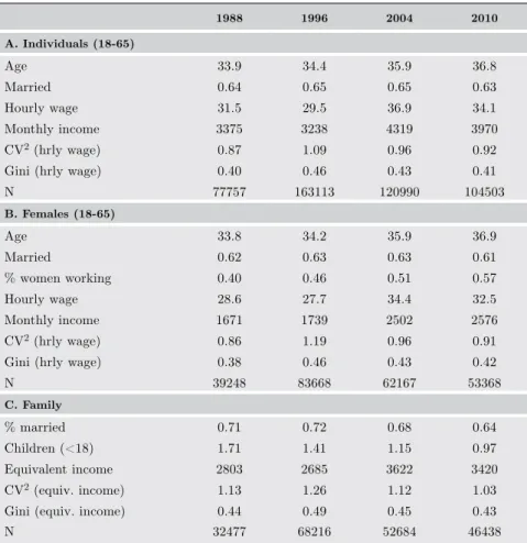
(12) 78. LATIN AMERICAN JOURNAL OF ECONOMICS | Vol. 49 No. 1 (May, 2012), 67–98. standard literature on wages and trim labor income to the 0.05 and 99.5 percentiles respectively. Income is adjusted for inflation and expressed in January 2010 pesos. We drop those individuals whose relationship with the household head is not specified and those with missing information about their education, age, marital status, and household head status. We also drop all households (and their members) that declare more than one head or more than one spouse.15 Additionally, we consider only households in which the head is at least 18 years old and less than 65 years old. Finally, we only use information on households in which at least one of its members reports positive income. Although zero income households may depend on nonmonetary income, the focus of our paper is on the effect of labor income on labor income inequality. Furthermore, the inclusion of these households that were not included does not affect our results. Comparing total income across all families may be inadequate due to family size scale ef fects. Most of the studies that deal with family income use a general equivalence scale to adjust for family size. Since the equivalence scale used in studies for other countries may not be suited for a developing country like Mexico, we use the equivalence scale published by CONEVAL.16 The equivalence scale gives a weight of 0.70 to individuals 0-5 years old, 0.74 to individuals 6-12 years old, 0.71 to individuals 13-17 years old, and 0.99 to the rest.17 Table 1 includes the number of observations at the individual and family level and descriptive statistics for 1988, 1996, 2004 and 2010. Panel A shows information at the individual level for the age group 18-65, Panel B corresponds to females and Panel C to families. Mean age has continuously increased over time from 33 to 36 years, the proportion of married individuals is constant until 2004 and there is a slight decline in marriage rates from 2004 to 2010. 18 The proportion of women working increases from 0.4 in 1988 to 0.57 in 2010. As in previous findings (Esquivel, 2009; Lopez-Acevedo, 2006), we can see that inequality follows an inverted,U-shaped pattern. This pattern is similar when we calculate inequality at the individual level, restrict 15. Dropped observations represent less than 3 percent of each year’s survey. 16. This government of fice is in charge of obtaining and reporting of ficial statistics on poverty rates in Mexico. http://www.coneval.gob.mx/ 17. Inequality trends are similar across different equivalence scales (per capita, square root of household size). 18. Marriage is defined as individuals married or cohabitating. If we define marriage by civil status, the decline in marriage rates is sharper..

(13) 79. R.M. Campos-Vazquez, A. Hincapie, and R.I. Rojas-Valdes | FAMILY INCOME INEQUALITY. Table 1. Descriptive statistics 1988. 1996. 2004. 2010. A. Individuals (18-65). Age. 33.9. 34.4. 35.9. 36.8. Married. 0.64. 0.65. 0.65. 0.63. Hourly wage. 31.5. 29.5. 36.9. 34.1. Monthly income. 3375. 3238. 4319. 3970. CV2 (hrly wage). 0.87. 1.09. 0.96. 0.92. Gini (hrly wage). 0.40. 0.46. 0.43. 0.41. 77757. 163113. 120990. 104503. N B. Females (18-65). Age. 33.8. 34.2. 35.9. 36.9. Married. 0.62. 0.63. 0.63. 0.61. % women working. 0.40. 0.46. 0.51. 0.57. Hourly wage. 28.6. 27.7. 34.4. 32.5 2576. Monthly income. 1671. 1739. 2502. CV2 (hrly wage). 0.86. 1.19. 0.96. 0.91. Gini (hrly wage). 0.38. 0.46. 0.43. 0.42. 39248. 83668. 62167. 53368. N C. Family. % married. 0.71. 0.72. 0.68. 0.64. Children (<18). 1.71. 1.41. 1.15. 0.97. Equivalent income. 2803. 2685. 3622. 3420. CV2 (equiv. income). 1.13. 1.26. 1.12. 1.03. Gini (equiv. income) N. 0.44. 0.49. 0.45. 0.43. 32477. 68216. 52684. 46438. Source: Authors’ calculations with data from INEGI. Notes: Sample restricted to urban households. Final sample excludes households with zero income and households in which the age of the household head is outside the range 18-65. Panel A uses information at the individual level, Panel B restricts the information to females and Panel C uses information at the family level. The term “married” in Panel C refers to families in which both husband and wife are currently cohabitating. Panel C equivalent income uses the equivalence scale provided by CONEVAL.. the calculation to females or calculate for the family level. Panel C shows that the proportion of married-couple families has not declined as much as the proportion of married individuals. The number of individuals under 18 years old has declined substantially in the last 20 years due to falling fertility rates. Mean income (adjusted by equivalence scales) decreased for the period 1988-1996 (due to the 1995 macroeconomic crisis) and then increased..

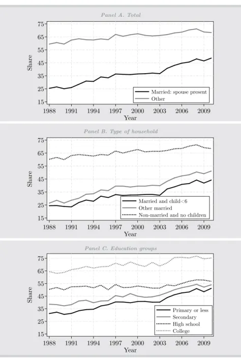
(14) 80. LATIN AMERICAN JOURNAL OF ECONOMICS | Vol. 49 No. 1 (May, 2012), 67–98. Figure 1. Urban household types: 1988-2010 80. Share. 60 Married: husband and wife Married: no spouse Single, divorced, etc. Singles living alone. 40 20 0 1988. 1991. 1994. 1997. 2000 Year. 2003. 2006. 2009. Source: Authors’ calculations with data from INEGI. Notes: Sample restricted to urban households. Final sample excludes households with zero income and households in which the age of the household head is outside the range 18-65. “Married: Husband & Wife” refers to both spouses living together in the household. “Married: no spouse” refers to families in which the household head declares that he or she is married but does not live with their spouse. “Single, Divorced, etc” refers to families in which the head of household declares their civil status as separated, divorced, or widowed with no cohabitation. “Singles living alone” refers to single persons who either live alone or are not related to the household head.. Figure 1 depicts the percentage of families in each of the four types previously described. The proportion of married-couple families has decreased 7 percentage points over the last 20 years. The percentage of households in which one spouse is not present, which represents only a small fraction (less than 2 percent) of the total, has barely changed. On the other hand, the number of families made up of one individual and those headed by divorced, separated, or widowed individuals has increased (driven mainly by single-parent families). Figure 2 shows family size for dif ferent types of families. For marriedcouple families, size has decreased approximately by one member in the last 20 years. This is mainly driven by decreases in fertility as evidenced by the number of members under 18 years old. On the other hand, family size for all other families has remained fairly constant at around two members per family. Figure 3 portrays the patterns of female labor supply for dif ferent groups. Panel A shows that the female labor supply increased more for married females than for non-married females. For example, married females increased their labor supply by more than 20 percentage points while for non-married females the rise is close to 10 percentage points..

(15) R.M. Campos-Vazquez, A. Hincapie, and R.I. Rojas-Valdes | FAMILY INCOME INEQUALITY. 81. Figure 2. Urban household size: 1988-2010 5. Number. 4 Household size: married Children <18: married Hosehould size: non-married. 3 2 1 1988. 1991. 1994. 1997. 2000 Year. 2003. 2006. 2009. Source: Authors’ calculations with data from INEGI. Notes: Sample restricted to urban households. Final sample excludes households with zero income and households in which the age of the household head is outside the range 18-65. Figure shows household size for urban households. “Children<18: Married” refers to the number of individuals under 18 years old living in married households.. Panel B shows the patterns of female labor supply for married females with children (under 6 years old) and other married females, as well as for non-married females with no children. The increase in the female labor supply was more pronounced among married females with no children. When we calculate labor supply by education group (Panel C), we find a rapid increase in female labor supply for individuals with low education.19 Females in the two lowest categories increased their labor supply more rapidly than females with high school or college degrees. Figure 4 shows the proportion of women working and mean married females’ income ranked by household income. The x-axis in both panels corresponds to the quintile of family equivalent income distribution without married females’ income. Panel A suggests that families with low family income had a higher proportion of married females working. However, as family income increases (quintile 2 and above), the percentage of working married females remained almost the same. There are some important dif ferences across time. From 1988 to 1996, there is a higher increase in the percentage of working married females. 19. We consider four schooling categories: less than secondary (less than nine years of schooling), complete secondary and incomplete high school (nine¡ to 11 years), complete high school and incomplete college (12 to 15 years), and complete college or more (16 years or more)..

(16) 82. LATIN AMERICAN JOURNAL OF ECONOMICS | Vol. 49 No. 1 (May, 2012), 67–98. Figure 3. Urban female labor supply: 1988-2010 Panel A. Total. 75 65. Share. 55 45 35 25 15 1988. Married: spouse present Other. 1991. 1994. 1997. 2000 Year. 2003. 2006. 2009. Panel B. Type of household. 75 65. Share. 55 45 35 Married and child<6 Other married Non-married and no children. 25 15 1988. 1991. 1994. 1997. 2000 Year. 2003. 2006. 2009. Panel C. Education groups. 75. Share. 65 55 45 35. Primary or less Secondary High school College. 25 15 1988. 1991. 1994. 1997. 2000 Year. 2003. 2006. 2009. Source: Authors’ calculations with data from INEGI. Notes: Sample restricted to urban households. Labor supply defined as individuals with positive hours of work. Panel A refers to female labor supply of married and non-married groups. Panel B is the same as Panel A but divides married females into females with children under 6 years old and others. Panel C refers to female labor supply for both married and non-married females by education groups..

(17) 83. R.M. Campos-Vazquez, A. Hincapie, and R.I. Rojas-Valdes | FAMILY INCOME INEQUALITY. Figure 4. Female labor supply and female income by household income in married and urban households: 1988-2010 Panel A. Female labor supply by household income. 70. 1988 1996 2004 2010. % working. 60 50 40 30 20. 1. 2. 3 Quintile. 4. 5. Panel B. Female income by household income. Mean income, female. 1200 1000 800 600 1988 1996 2004 2010. 400 200 1. 2. 3 Quintile. 4. 5. Source: Authors’ calculations with data from INEGI. Notes: Sample restricted to urban households. Final sample excludes households with zero income and households in which the age of the household head is outside the range 18-65. Furthermore, sample is restricted to married households (both husband and wife living together) with positive income. Panel A refers to female labor supply according to the quintile of the income distribution for the rest of the household (total family income less wife’s income). Income is adjusted using equivalence scales as described in the text. Panel B refers to mean female income according to the quintile income distribution for the rest of household’s income. Income is in real terms (January 2010 pesos).. in high-income households than working married females in middleincome households. After 1996, married females in quintiles 1 to 4 increased their labor force participation more than those in quintile 5. Panel B shows the mean of the wife’s income for each quintile of the family income distribution. It shows that mean income in quintile 1.

(18) 84. LATIN AMERICAN JOURNAL OF ECONOMICS | Vol. 49 No. 1 (May, 2012), 67–98. was higher than in quintile 2 due to the high attachment of married females to the labor market. Married females in wealthy families earned relatively more than in families in quintiles 2 to 4. In general, Figure 4 shows that women married to men in quintile 5 have not increased their labor supply as other married females have after 1996. Moreover, from 1988 to 1996 there was a marked increased in earnings for married females in high-income households. Also, in the period 1996-2010 there was a higher relative increase in income for married females in quintiles 1-4 than that for married females in quintile 5. In sum, previous results show that the female labor supply has increased over the last 20 years, with particularly significant rises for married females and females with low levels of education. Additionally, married females in high-income families increased their labor force participation and earnings relatively more during the period 1988-1996 than in 1996-2010. The following sections show the formal calculations carried out to investigate the effect of married females’ income on family income inequality.. 5.. Results. In this section, we show the calculations of the counterfactual analysis described in Section 3. The key parts of these decompositions are the share of income of married females and married males and the correlation between income sources. Figure 5 shows these key elements among married-couple families. The income share of married males in 1988 was 73 percent while in 2010 it was 64 percent. At the same time, the income share of married females increased 10 percentage points (from 13 percent in 1988 to 23 percent in 2010). The income share of other members in the household didn’t change over the 20 years. Although the income share for married females in the 2000s is similar to previous findings in countries such as Spain, Greece and Italy (Pasqua, 2008; Harkness, 2010), it was still substantially lower than in countries such as Denmark and Sweden.20 Panel B in Figure 5 shows that the correlation among income sources has barely changed in the last 20 years. Although the correlations fluctuate every year, the long-run relationships are stable. The correlation between married males’ and married females’ income is positive and, on average across time, equal to 0.28 (in 1988 it is equal to 0.27 and in 2010 it is equal to 0.28). This number is high in comparison to the results of studies 20. Pasqua (2008) reports a female income share among married couples of 34.5 percent in Denmark and 30.8 percent in Sweden..

(19) R.M. Campos-Vazquez, A. Hincapie, and R.I. Rojas-Valdes | FAMILY INCOME INEQUALITY. 85. Figure 5. Share of income and correlations among urban married families: 1988-2010. Share of income. Panel A. Share of income. 90 80 70 60. Husbands Wives Others. 50 40 30 20 10 0 1988. 1991. 1994. 1997. 2000 Year. 2003. 2006. 2009. Correlation coefficient. Panel B. Correlations. 0.35 0.30 0.25 0.20 0.15 0.10 0.05 0.00 -0.05 -0.10 1988. Husbands and wives Husbands and others Wives and others. 1991. 1994. 1997. 2000 Year. 2003. 2006. 2009. Source: Authors’ calculations with data from INEGI. Notes: Sample restricted to urban households. Final sample excludes households with zero income and households in which the household head age is outside the range 18-65. Furthermore, sample is restricted to married households. Panel A measures the share of income of each source and Panel B shows the correlation of income sources.. for other countries. For the U.S., Cancian and Reed (1999) found that the correlation between married males’ and married females’ income was close to 0.22 in 1994, and they also showed an increase in the correlation equal to 0.10 from 1967 to 1994. Moreover, Del Boca and Pasqua (2003) found that the correlation in Italy in 1998 was 0.21, although they showed a correlation of 0.26 for Northern Italy. Also, Pasqua (2008) showed that the correlation between married males’ and married females’ income across.

(20) 86. LATIN AMERICAN JOURNAL OF ECONOMICS | Vol. 49 No. 1 (May, 2012), 67–98. OECD countries was fairly low and close to zero; only Portugal had a correlation close to 0.30. Amin and Da Vanzo (2004) found a correlation value equal to 0.13 in 1988 in Malaysia. Hence, a correlation of 0.28 is higher than those in the U.S., Italy, Malaysia and most OECD countries. As far as we are concerned, this result for Mexico was not previously known. On the other hand, both the correlation of married males’ and other sources’ income and the correlation of married females’ and others sources’ income are close to -0.08. Figure 6. Coef ficient of variation, urban areas: 1988-2010 Panel A. Individuals. Coefficient of variation (base year 1988). 0.30 0.15 0.00 -0.15 -0.30 1988. Total Males Females. 1991. 1994. 1997. 2000 Year. 2003. 2006. 2009. Panel B. Individual vs. household inequality. Coefficient of variation (base year 1988). 0.30 0.15 0.00 -0.15 -0.30 1988. Individual Household. 1991. 1994. 1997. 2000 Year. 2003. 2006. 2009. Source: Authors’ calculations with data from INEGI. Notes: Sample restricted to urban households. Base year is 1988. Individual inequality sample restricted to individuals between 18 and 65 years old. Household inequality sample excludes households with zero income and households in which the age of the household head is outside the range 18-65. We use total labor income for the inequality calculations. Hourly wage inequality follows a similar trend..

(21) R.M. Campos-Vazquez, A. Hincapie, and R.I. Rojas-Valdes | FAMILY INCOME INEQUALITY. 87. Figure 7. Coef ficient of variation by type of family, urban areas: 1988-2010. Coefficient of variation. Panel A. Married households. 3.2 2.6 2.0 Husbands Wives Others Non-married. 1.4 0.8 1988. 1991. 1994. 1997. 2000 Year. 2003. 2006. 2009. Panel B. All households. Coefficient of variation. 1.4 1.2 1.0 0.8 0.6 1988. Total Married Non-married. 1991. 1994. 1997. 2000 Year. 2003. 2006. 2009. Source: Authors’ calculations with data from INEGI. Notes: Sample restricted to urban households. Final sample excludes households with zero income and households in which the age of the household head is outside the range 18-65. Panel A shows the coef ficient of variation of each income source for married households. Panel B shows the coef ficient of variation by type of household.. Figure 6 shows trends in inequality at the individual and household levels. In order to analyze income inequality trends, we normalize the coefficient of variation by its 1988 level. Panel A shows an increase in inequality for all individuals, males and females for the period 19881996. After 1996, we observe a decline in inequality with the exception of years 2000-2001. In Panel B, inequality at the individual or household.

(22) 88. LATIN AMERICAN JOURNAL OF ECONOMICS | Vol. 49 No. 1 (May, 2012), 67–98. level follows a similar pattern. Since male inequality turns out to be the main determinant for individual income inequality, male inequality is more similar to household inequality than female inequality. In fact, Panel A shows that female income inequality has not decreased as much as male inequality since 2002. In sum, inequality follows an inverted U-shape pattern both at the individual and the household level. Although the patterns of individual income inequality are important for illustrating the similarity between individual and household inequality, the main goal of the paper is to analyze the contribution of married females’ earnings to total household inequality. Following the decomposition in equations (1) and (2), Figure 7 shows the evolution of family income inequality using the coef ficient of variation for each source of income among married-couple families and for all families. Panel A shows inequality for married males, married females, other sources and families formed of unmarried individuals. Inequality decreases most for married males and married females. Inequality for other sources barely changed and inequality for unmarried individuals slightly decreased for the period 1996-2010.21 Panel B shows the pattern of inequality for both married-couple and non-married-couple families. Inequality for married-couple families decreased substantially after 1996. In general, figures 6 and 7 show an inverted U-shaped pattern in family income inequality during the period 1988-2010. This pattern is robust to changes in the inequality index.22 Following are the results of the counterfactual computations described in Section 3. Each counterfactual facilitates our understanding of the role of married females’ earnings in inequality. First, we calculate the contribution of married males’ income inequality using Equation (1). In particular, we fix all parameters to their 1988 levels and only allow male inequality to change. Then we analyze the contribution of married females, i.e., the income share and income inequality of married females. By first varying the share of income before female inequality, we simulate the ef fect of higher income for women who were participating in the labor market in 1988. However, the female labor supply increased after that year, especially for women in poor families. Hence, we expect an increase in inequality with this counterfactual as 21. We have also calculated inequality by gender and marital status, but these results are not shown. Inequality decreased the most for married males and then for non-married males in the period 2000-2010. Inequality for non-married females increased the most during the period 1990-1999. 22. See the results from Esquivel (2009), Esquivel, Lustig, and Scott (2010), Lopez-Calva and Lustig (2010), López-Acevedo (2006) and Campos-Vazquez (2010)..

(23) R.M. Campos-Vazquez, A. Hincapie, and R.I. Rojas-Valdes | FAMILY INCOME INEQUALITY. 89. Figure 8. Counterfactual distributions, urban areas: 1988-2010 Panel A. Married households one component at a time. Coefficient of variation. 0.4. Observed CV males +Shares +CV females. 0.2. 0.0. -0.2 1988. 1991. 1994. 1997. 2000 Year. 2003. 2006. 2009. Panel B. All households - marriage rates constant. Coe cient of variation. 0.4. 0.2. 0.0. -0.2 1988. Observed CV males +CV females and shares +Rho free. 1991. 1994. 1997. 2000 Year. 2003. 2006. 2009. Source: Authors’ calculations with data from INEGI. Notes: Sample restricted to urban households. Final sample excludes households with zero income and households in which the age of the household head is outside the range 18-65. Results are presented using 1988 as the base year (both observed and counterfactual inequality start at zero in 1988).. women from poor families increase their labor supply and Equation (1) assumes the “same women” as in 1988 are increasing their share of income. Because it is dif ficult to separate the net ef fect of female labor supply from both Sw2 and CVw2, we argue that the combined ef fect is the contribution of married females to family income inequality. The dif ference between the last counterfactual (combined ef fect of married males and females) and observed inequality is the contribution of the rest of the parameters, i.e., correlations of earnings among members of the family and inequality of residual income. Finally, we can use.

(24) 90. LATIN AMERICAN JOURNAL OF ECONOMICS | Vol. 49 No. 1 (May, 2012), 67–98. Figure 9. Robustness test: Average contribution of all counterfactuals, married households. Contribution to CV. 0.4. Observed Males Females Rhos and residual. 0.2. 0.0. -0.2 1988. 1991. 1994. 1997. 2000 Year. 2003. 2006. 2009. Source: Authors’ calculations with data from INEGI. Notes: Sample restricted to urban households. Final sample excludes households with zero income and households in which the age of the household head is outside the range 18-65. Results are presented using 1988 as the base year (both observed and counterfactual inequality start at zero in 1988).. Equation (2) to calculate the ef fect of marriage rates on total income inequality. In particular, we calculate inequality among married households from the previous counterfactuals, fix the marriage rate to its 1988 level and let inequality vary among non-married households. Figure 8 shows the main results. In Panel A we plot observed inequality and inequality for each counterfactual with the following ordering using Equation (1): 1. CVw2, 2. Sw2 3. CVw2. Panel B plots inequality among all households using Equation (2), with the marriage rate fixed to its 1988 value but allowing inequality of non-married households change as it did. In Panel A, we observe that even when fixing all parameters to their 1988 value, the main determinant of family inequality is married male inequality.23 This is consistent with a larger share corresponding to husbands’ income. As males are the breadwinners of the households in our sample, inequality of married males is the main determinant of family income inequality. Next we show the ef fect of varying both CVm2 and Sw2 (the line that says “+Shares”). We observe an increase in family inequality especially in the 2000-2010 decade. This is consistent with the recent increase in 23. Using the initial year as the base year is more intuitive than using others. However, our results are robust to using other years as the base year. When we recalculated all statistics (unreported) using base years 1996 and 2010, the interpretation of the results does not change..

(25) R.M. Campos-Vazquez, A. Hincapie, and R.I. Rojas-Valdes | FAMILY INCOME INEQUALITY. 91. female labor supply among poor families. Allowing an increase in the share of income of married females is equivalent to saying that the “same women” who were participating in 1988 are participating each year but with a larger share of income. When CVm2, Sw2 and CVw2 in Equation (1) change as they did and the rest of the parameters are fixed to their 1988 levels, we calculate the net ef fect of the increase in female labor supply and the change in the wage structure. Indeed, Panel A shows that inequality decreases and is very similar to observed inequality, which means that the rest of the parameters are relatively unimportant in explaining changes in inequality. Panel A summarizes the main results of the paper. First, married male income inequality is the main determinant of family income inequality. Second, both the labor supply and wage structure of married females contribute to a decrease in family income inequality. Finally, the correlation of earnings within the family has virtually no ef fect on inequality. Using data from all households and the previous counterfactuals, Panel B shows the ef fect of marriage rates on total inequality. We observe that had marriage rates remained constant at their 1988 level, total inequality would have been lower. One critique of the decomposition exercise is that order matters. It is possible that the magnitude of the contribution of each component would change if we reverse the ordering. Hence, in order to analyze this possible effect among married households, we calculate the average contribution of married males, females (both share of income and inequality) and other components. The results are presented in Figure 9. The figure shows that the contributions of each component in Figure 8 are robust to the ordering. Male inequality is the main determinant of family income inequality. Married females contribute to equalizing family income distribution in the decade 2000-2010. If the female labor supply had not changed, family income inequality would have been higher. Finally, the contribution of the correlation of earnings and residual income to family inequality is practically zero.. 6.. How do females af fect income distribution?. The previous section showed that married female earnings contribute to equalizing income distribution. In Section 4 we showed that the female labor supply has increased over time, especially for married females (figures 3 and 4). We also showed that female labor supply.

(26) 92. LATIN AMERICAN JOURNAL OF ECONOMICS | Vol. 49 No. 1 (May, 2012), 67–98. increased more for low-skilled groups. In this section, we briefly analyze how married females af fect the income distribution. Table 2. Female statistics 1988. 1996. 2004. 2010. % Families: husband & wife work. 0.232. 0.3. 0.369. 0.431. % Families: husband works only. 0.678. 0.625. 0.566. 0.486. % Families: wife works only. 0.020. 0.032. 0.035. 0.054. % Married females with full-time job. 0.123. 0.172. 0.233. 0.275. % Married females with part-time job. 0.116. 0.143. 0.152. 0.193. % Non-married with full-time job. 0.408. 0.434. 0.469. 0.471. % Non-married with part-time job. 0.153. 0.173. 0.173. 0.193. Correlation of married males' hours & married females' hours of work. 0.029. -0.003. -0.014. -0.011. Correlation of married males' income & married females' hours of work. -0.007. -0.003. -0.006. -0.03. Age of husband (restricted to working married males). 38.9. 39.2. 40.7. 42.3. Age of wife if she is working. 35.2. 36.5. 38.3. 39.8. Age of wife if she is not working. 36.2. 36.2. 37.9. 39.6. % of families w/both husband & wife working (first quartile of income distribution excluding married females' income). 0.212. 0.273. 0.356. 0.425. % of families w/both husband & wife working (fourth quartile of income distribution excluding married females' income). 0.242. 0.351. 0.411. 0.464. Wives’ income share (first quartile). 0.155. 0.243. 0.282. 0.414. Wives’ income share (fourth quartile). 0.082. 0.096. 0.112. 0.131. Source: Authors’ calculations with data from INEGI. Notes: Sample restricted to urban households. Final sample excludes households with zero income and households in which the age of the household head is outside the range 18-65. Work in all rows is defined as positive hours of work. Full-time is defined as individuals working more than 35 hours per week, while part-time is those individuals working positive hours but less than 35 hours per week. The last four rows in the table are obtained by sorting the data according to family equivalent income minus the wife's equivalent income.. Table 2 shows how dif ferent characteristics have evolved over time. As previously shown, married females have increased their labor supply over time. However, this could be due to an increase in non-working married males. The first three rows in the table present the percentage of families according to the employment status of the husband and wife. Indeed, the percentage of families in which both husband and wife work has been growing in the last 20 years. The percentage of.

(27) R.M. Campos-Vazquez, A. Hincapie, and R.I. Rojas-Valdes | FAMILY INCOME INEQUALITY. 93. families in which both husband and wife worked in 1988 was 23 percent, but by 2010 this figure had risen to 43 percent. The next three rows show that the increase in female labor supply is mainly due to work in full-time jobs, especially for married females. Is this increase in the female labor supply related to changes in married males’ income or married males’ working hours? Results presented in Table 2 show that this is not the case. Both correlations (rows 8 and 9) are close to zero. Hence, the increase in the female labor supply does not seem to be related to changes in married males’ employment conditions. It is also possible that the increase in married females’ labor supply is due to the existence of new cohorts. If this is the case, we should observe a decrease or a dif ferentiated pattern in age between married females who work and those who do not work. However, Table 2 shows that changes in average age over time for married females who work and those who do not work are very similar. This suggests that the increase in the female labor supply is not restricted to younger cohorts. Table 2 also shows the percentage of families in which both husband and wife work, in relation to a specified quartile of the income distribution (excluding married females’ income). This percentage increases more for wealthier families during the period 1988-1996. However, the gap diminishes in the period 1996-2010. The percentage of families in which both husband and wife work in the first quartile by 15 percentage points during 1996-2010, while for the fourth quartile it only rises by 11 percentage points. Moreover, the last two rows in the table show a marked increase in the share of income contributed by married females in poor families (first quartile), growing from 13 percent in 1988 to 41 percent in 2010.24 Based on these findings and also those shown in figures 3 and 4, we consider that the increase in married females’ labor supply, especially in low-income families, has contributed to the decrease in family income inequality.25. 24. The increased share of income may be due to a higher proportion of non-working husbands. When we exclude all families with zero income except for married females’ income, we get similar results. In this case, wives’ income share in 1988 is 8.8 percent and 8.2 percent in the first and fourth quartile respectively, while in 2010 we obtain 16.1 percent and 12.9 percent in the first and fourth quartile respectively. Hence, even when we exclude families with zero income (except for wives’ income) we observe a higher increase in income among poorer families. 25. In fact, the percent of households with wives working and husbands not working has increased over time. This process suggests an added worker ef fect which is consistent with findings in Parker and Skoufias (2004, 2006)..

(28) 94. 7.. LATIN AMERICAN JOURNAL OF ECONOMICS | Vol. 49 No. 1 (May, 2012), 67–98. Conclusions. Income inequality in Mexico has followed an inverted U-shaped pattern over the last 25 years. At the same time, female labor force participation increased substantially, especially among low-skilled female workers. For this period, we analyze whether changes in married females’ earnings in married-couple families and changes in marriage rate had an equalizing ef fect on family income distribution. Using data from urban areas in Mexico for the period 1988-2010, we compare observed family income inequality (using equivalence scales) with counterfactual distributions under a number of dif ferent assumptions. Among maried households, we find that married male income inequality is the main determinant of family income inequality. Second, both the female labor supply and the wage structure of married females contribute to a decrease in family income inequality. Finally, the correlation of earnings within the family does not af fect income inequality. On the other hand, for all households, had marriage rates remained at the 1988 level, inequality would have been lower. Although the female labor supply grows for all groups, the increase is higher for married females, low-skilled females, and married females in poor families. We also find that the correlation between married males’ and married females’ earnings has been fairly stable at around 0.28 which is one of the highest values recorded in similar studies in other countries. Therefore, we consider that family income inequality did not fall because of a reduction in income assortative mating; rather, this decrease is driven by the increment in married females’ labor supply among poor households and also by a reduction of inequality among the partners of females. One final caution should be noted. We consider the ef fect of market female labor supply but do not take into account the importance of home production. Our data does not allow us to verify whether the total number of hours of work for married females (market plus home production) has changed over time. Hence, we are unable to discern possible welfare ef fects at the family level. Although the welfare ef fects on families are beyond the scope of our paper, it may be the case that increasing participation of married females in the labor market occurs at the expense of their leisure time, if married females remain largely responsible for housework and childcare. Moreover, we do not address the behavioral components of the ef fect of married males’ labor supply.

(29) R.M. Campos-Vazquez, A. Hincapie, and R.I. Rojas-Valdes | FAMILY INCOME INEQUALITY. 95. on married females’ earnings or the ef fects of household structure on inequality or labor participation. Future research is needed in order to address these issues..

(30) 96. LATIN AMERICAN JOURNAL OF ECONOMICS | Vol. 49 No. 1 (May, 2012), 67–98. REFERENCES Amin, S. and J. DaVanzo, (2004), “The impact of wives’ earnings on earnings inequality among married-couple households in Malaysia,” Journal of Asian Economics, Vol. 15, No. 1: 49-70. Aslaksen, I., T. Wennemo, and R. Aaberge (2005), “Birds of a feather flock together: The impact of choice of spouse on family labor income inequality,” Labour, Vol. 19, No. 3: 491-515. Bosch, M. and M. Manacorda (2008), “Minimum wages and earnings inequality in urban Mexico: Revisiting the evidence,” CEP Discussion Paper 880, Centre for Economic Performance, London. Campos-Vazquez, R.M. (2010). “Why did wage inequality decrease in Mexico after NAFTA?” Serie Documentos de Trabajo 15, El Colegio de México, Centro de Estudios Económicos, Mexico City. Cancian, M. and D. Reed (1998), “Assessing the ef fects of wives’ earnings on family income inequality,” The Review of Economics and Statistics, Vol. 80, No. 1: 73-79. Cancian, M. and D. Reed (1999), “The impact of wives’ earnings on income inequality: Issues and estimates,” Demography, Vol. 36, No. 2: 173-184. Cragg, M. and M. Epelbaum (1996), “Why has wage dispersion grown in Mexico? Is it the incidence of reforms or the growing demand for skills?” Journal of Development Economics, Vol. 51, Vol. 1: 99-116. Daly, M.C. and R.G. Valleta (2006), “Inequality and poverty in the United States: The ef fects of rising dispersion of men’s earnings and changing family behavior,” Economica, Vol. 73, No. 289: 75-98. Davies, H. and H. Joshi (1998), “Gender and income inequality in the UK 19681990: The feminization of earnings or of poverty?” Journal of the Royal Statistical Society, Series A (Statistics in Society), Vol. 161, No. 1: 33-61. Del Boca, D. and S. Pasqua (2003), “Employment patterns of husbands and wives and family income distribution in Italy (1977-98).” Review of Income and Wealth, Vol. 49, No. 2: 221-245. DiNardo, J., N.M. Fortin, and T. Lemieux (1996), “Labor market institutions and the distribution of wages, 1973-1992: A semiparametric approach,” Econometrica, Vol. 64, No. 5: 1001-1044. Esquivel, G. (2009). “The dynamics of income inequality in Mexico since NAFTA.” Regional Bureau for Latin America and the Caribbean Research for Public Policy Inclusive Development Working Paper ID-02-2009, United Nations Development Programme, New York. Esquivel, G., N. Lustig, and J. Scott (2010). “Mexico: A decade of falling inequality: Market forces or State action?” in L. F. Lopez-Calva, and N. Lustig, eds., Declining inequality in Latin America. A Decade of Progress? Washington, D.C.: Brookings Institution. Esquivel, G. and J.A. Rodríguez-López (2003), “Technology, trade and wage inequality,” Journal of Development Economics, Vol. 72, No. 2: 543-565..

(31) R.M. Campos-Vazquez, A. Hincapie, and R.I. Rojas-Valdes | FAMILY INCOME INEQUALITY. 97. Fairris, D. (2003), “Unions and wage inequality in Mexico,” Industrial and Labor Relations Review, Vol. 56, No. 3: 481-497. Ferreira, F., D. De Ferranti, G.E. Perry, and M. Walton (2004), Inequality in Latin America: Breaking with history? (Washington, D.C.: The World Bank). García, B. (2001), “Reestructuración económica y feminización del mercado de trabajo en México,” Papeles de Población, Vol. 27: 45-61. Gottschalk, P. and S. Danziger, S. (2005). “Inequality of wage rates, earnings and family income in the United States, 1975-2002.” Review of Income and Wealth, 51(2), pp. 231-254. Harkness, S. (2010), “The contribution of women’s employment and earnings to household income inequality: A cross country analysis,” Luxembourg Income Survey, Working Paper Series 531, Luxembourg. Johnson, D. and R. Wilkins (2004), “Ef fects of changes in family composition and employment patterns on the distribution of income in Australia: 1981-1982 to 1997- 1998.” Economic Record, Vol. 80, No. 249: 219-238. Juhn, C. and K.M. Murphy (1997), “Wage inequality and family labor supply,” Journal of Labor Economics, Vol. 15, No. 1: 72-97. Katz, L. and D. Autor (1999), “Changes in the wage structure and earnings inequality,” in O. Ashenfelter and D. Card, eds., Handbook of Labor Economics, Vol. 3C: 1463-1555. Lehrer, E.L. (2000), “The impact of women’s employment on the distribution of earnings among married-couple households: A comparison between 1973 and 1992-1994,” The Quarterly Review of Economics and Finance, Vol. 40, No. 3: 295-301. Lopez, J.H. and G. Perry (2008), “Inequality in Latin America: Determinants and consequences,” Policy Research Working Paper 4504, The World Bank, Washington, D.C. Lopez-Calva, L. F., and N. Lustig (2009), “The recent decline of inequality in Latin America: Argentina, Brazil, Mexico and Peru.” Working Papers 140, ECINEQ, Society for the Study of Economic Inequality, Palma de Mallorca. Lopez-Calva, L.F. and N. Lustig, (2010), “Explaining the decline in inequality in Latin America: Technological change, educational upgrading and democracy,” in L. F. Lopez-Calva and N. Lustig, eds., Declining Inequality in Latin America. A Decade of Progress? Washington, D.C.: Brookings Institution. López-Acevedo, G. (2006), “Mexico: Two decades of the evolution of education and inequality,” World Bank Policy Research Working Paper 3919, The World Bank, Washington, D.C. Machado, J.A.F. and J. Mata (2005), “Counterfactual decomposition of changes in wage distributions using quantile regression,” Journal of Applied Econometrics, Vol. 20, No. 4: 445-465. Machin, S. (2008), “An Appraisal of Economic Research on Changes in Wage Inequality.” Labour, Vol. 22 (Special Issue): 7-26. Martin, M.A. (2006), “Family structure and income inequality in families with children, 1976 to 2000,” Demography, Vol. 43, No. 3: 421-445..

(32) 98. LATIN AMERICAN JOURNAL OF ECONOMICS | Vol. 49 No. 1 (May, 2012), 67–98. McKenzie, D.J. (2003). “How do households cope with aggregate shocks? Evidence from the Mexican peso crisis,” World Development, Vol. 31, No. 7: 1179-1199. Parker, S. and E. Skoufias (2004), “The added worker ef fect over the business cycle: Evidence from urban Mexico,” Applied Economic Letters, Vol. 11, No. 10: 625-630. Parker, S. and E. Skoufias (2006), “Job loss and family adjustment in work and schooling during the Mexican peso crisis,” Journal of Population Economics, Vol. 19, No. 1: 163-181. Pasqua, S. (2008), “Wives’ work and income distribution in European countries,” European Journal of Comparative Economics, Vol. 5, No. 2: 157-186. Rendón, T. (2003), “Empleo, segregación y salarios por género,” in E. de la Garza Toledo, and C. S. Páez, eds., La Situación del Trabajo en México, México City: Plaza y Valdés. Robertson, R. (2007), “Trade and wages: Two puzzles from Mexico,” The World Economy, Vol. 9, No. 30: 1378-1398. Sotomayor, O.J. (2009), “Changes in the distribution of household income in Brazil: The role of male and female earnings,” World Development, Vol. 37, No. 10: 1706-1715. Wong, R. and R.E. Levine (1992), “The ef fect of household structure on women’s economic activity and fertility: Evidence from recent mothers in urban Mexico,” Economic Development and Cultural Change, Vol. 41, No. 1: 89-102..

(33)