The Chandra Cosmos Legacy Survey: Overview and Point Source Catalog

Texto completo

(1)The Astrophysical Journal, 819:62 (18pp), 2016 March 1. doi:10.3847/0004-637X/819/1/62. © 2016. The American Astronomical Society. All rights reserved.. THE CHANDRA COSMOS LEGACY SURVEY: OVERVIEW AND POINT SOURCE CATALOG F. Civano1,2, S. Marchesi1,2,3, A. Comastri4, M. C. Urry1, M. Elvis2, N. Cappelluti4, S. Puccetti5, M. Brusa3,4, G. Zamorani4, G. Hasinger6, T. Aldcroft2, D. M. Alexander7, V. Allevato8, H. Brunner9, P. Capak10,11, A. Finoguenov8, F. Fiore12, A. Fruscione2, R. Gilli4, K. Glotfelty2, R. E. Griffiths13, H. Hao2, F. A. Harrison14, K. Jahnke15, J. Kartaltepe16,17, A. Karim18, S. M. LaMassa1, G. Lanzuisi3,4, T. Miyaji19,20, P. Ranalli21, M. Salvato9, M. Sargent22, N. J. Scoville11, K. Schawinski23, E. Schinnerer15,24, J. Silverman25, V. Smolcic26, D. Stern27, S. Toft28, B. Trakhenbrot23, E. Treister29, and C. Vignali3,4 1. Yale Center for Astronomy and Astrophysics, 260 Whitney Avenue, New Haven, CT 06520, USA 2 Harvard-Smithsonian Center for Astrophysics, 60 Garden Street, Cambridge, MA 02138, USA Dipartimento di Fisica e Astronomia, Università di Bologna, viale Berti Pichat 6/2, I-40127 Bologna, Italy 4 INAF–Osservatorio Astronomico di Bologna, via Ranzani 1, I-40127 Bologna, Italy 5 ASDC–ASI, Via del Politecnico, I-00133 Roma, Italy 6 Institute for Astronomy, 2680 Woodlawn Drive, University of Hawaii, Honolulu, HI 96822, USA 7 Centre for Extragalactic Astronomy, Department of Physics, Durham University, South Road, Durham DH1 3LE, UK 8 Department of Physics, University of Helsinki, Gustaf Hällströmin katu 2a, FI-00014 Helsinki, Finland 9 Max-Planck-Institut für extraterrestrische Physik, Giessenbachstrasse 1, D-85748 Garching bei München, Germany 10 Infrared Processing and Analysis Center (IPAC), 1200 East California Boulevard, Pasadena, CA 91125, USA 11 California Institute of Technology, 1200 East California Boulevard, Pasadena, CA 91125, USA 12 INAF—Osservatorio Astronomico di Roma, via Frascati 33, Monte Porzio Catone, I-00040, Italy 13 Physics & Astronomy Dept., Natural Sciences Division, University of Hawaii at Hilo, 200 W. Kawili St., Hilo, HI 96720, USA 14 Cahill Center for Astronomy and Astrophysics, California Institute of Technology, 1216 E. California Blvd, Pasadena, CA 91125 USA 15 Max Planck Institute for Astronomy, Koenigstuhl 17, D-69117 Heidelberg, Germany 16 National Optical Astronomy Observatory, 950N. Cherry Ave, Tucson AZ 85719, USA 17 School of Physics and Astronomy, Rochester Institute of Technology, 84 Lomb Memorial Dr., Rochester, NY 14623, USA 18 Argelander-Institut für Astronomie, Universität Bonn, Auf dem Hügel 71, D-53121 Bonn, Germany 19 Instituto de Astronomía sede Ensenada, Universidad Nacional Autónoma de México, Km. 103, Carret. Tijunana-Ensenada, Ensenada, BC, Mexico 20 University of California San Diego, Center for Astrophysics and Space Sciences, 9500 Gilman Drive, La Jolla, CA 92093-0424, USA 21 AASARS, National Observatory of Athens, 15236 Penteli, Greece 22 Astronomy Centre, Department of Physics and Astronomy, University of Sussex, Brighton, BN1 9QH, UK 23 Institute for Astronomy, Department of Physics, ETH Zurich, Wolfgang-Pauli-Strasse 27, CH-8093 Zurich, Switzerland 24 National Radio Astronomy Observatory, Pete V. Domenici Science Operations Center, 1003 Lopezville Road, Socorro, NM 87801, USA 25 Kavli Institute for the Physics and Mathematics of the universe (Kavli IPMU, WPI), Todai Institutes for Advanced Study, The University of Tokyo, Kashiwa 2778583, Japan 26 Department of Physics, University of Zagreb, Bijenička cesta 32, HR-10000 Zagreb, Croatia 27 Jet Propulsion Laboratory, California Institute of Technology, 4800 Oak Grove Drive, Pasadena, CA 91109, USA 28 Dark Cosmology Centre, Niels Bohr Institute, University of Copenhagen, Juliane Mariesvej 30, DK-2100 Copenhagen, Denmark 29 Universidad de Concepción, Departamento de Astronomía, Casilla 160-C, Concepción, Chile Received 2015 July 31; accepted 2015 December 24; published 2016 February 29 3. ABSTRACT The COSMOS-Legacy survey is a 4.6 Ms Chandra program that has imaged 2.2 deg2 of the COSMOS field with an effective exposure of 160 ks over the central 1.5 deg2 and of 80 ks in the remaining area. The survey is the combination of 56 new observations obtained as an X-ray Visionary Project with the previous C-COSMOS survey. We describe the reduction and analysis of the new observations and the properties of 2273 point sources detected above a spurious probability of 2×10−5. We also present the updated properties of the C-COSMOS sources detected in the new data. The whole survey includes 4016 point sources (3814, 2920 and 2440 in the full, soft, and hard band). The limiting depths are 2.2×10−16, 1.5×10−15, and 8.9×10−16 erg cm-2 s-1 in the 0.5–2, 2–10, and 0.5–10 keV bands, respectively. The observed fraction of obscured active galactic nuclei with a column +17 density >1022 cm−2 from the hardness ratio (HR) is ∼5016 %. Given the large sample we compute source number counts in the hard and soft bands, significantly reducing the uncertainties of 5%–10%. For the first time we compute number counts for obscured (HR>−0.2) and unobscured (HR<−0.2) sources and find significant differences between the two populations in the soft band. Due to the unprecedent large exposure, COSMOS-Legacy area is three times larger than surveys at similar depths and its depth is three times fainter than surveys covering similar areas. The area-flux region occupied by COSMOS-Legacy is likely to remain unsurpassed for years to come. Key words: catalogs – cosmology: observations – galaxies: evolution – quasars: general – surveys – X-rays: general Supporting material: machine-readable table. 1. INTRODUCTION. when the universe was less than ∼0.6 Gyr old), where the growth of structures becomes highly nonlinear and the first stars form, and z∼2 (∼3.25 Gyr old), where major. One of the most active but least-known epochs in astrophysics is the period between reionization (z  8, i.e., 1.

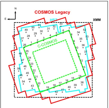
(2) The Astrophysical Journal, 819:62 (18pp), 2016 March 1. Civano et al.. virialization occurs and star formation (SF) and supermassive black hole (SMBH) accretion peak. At these early times the precursors of the clusters and groups seen at z1 have low density and are much larger on both physical (Mpc) and observed (arcminutes) scales. Surveys for these large-scale structures become rapidly more efficient as the dimension of the survey exceeds the structure’s typical sizes (∼15′). Large area surveys (several times 15′ wide) are essential for the detection of these structures, which cannot be seen in smaller area surveys, however deep. The equatorial 2 deg2 COSMOS area (Scoville et al. 2007a) is the deepest, most complete survey accessible to both hemispheres (notably by both ALMA and the Karl G. Jansky VLA) and is large enough to find high redshift clusters. A significant investment of 640 Hubble Space Telescope (HST) orbits (Koekemoer et al. 2007, Scoville et al. 2007b), 620h of Spitzer (P. Capak et al. 2016, in preparation30), 260h of Herschel (Lutz et al. 2011), 750 hr of JVLA (Schinnerer et al. 2004, 2007, 2010 and V. Smolcic et al. 2016 in preparation), over 300 nights of large ground-based telescopes VLT, Keck, Subaru, VISTA for both imaging and spectroscopy (Taniguchi et al. 2007; Lilly et al. 2009) have been made in this field. The first homogeneous coverage in the X-rays of the whole COSMOS field was obtained with the XMM-Newton satellite (1.5 Ms; Hasinger et al. 2007; Cappelluti et al. 2009; Brusa et al. 2010). These observations have been crucial for characterizing the most luminous Active Galactic Nuclei (AGNs) in COSMOS (e.g., Brusa et al. 2010; Allevato et al. 2011; Mainieri et al. 2011; Lusso et al. 2012 among others). The obscured AGN population of the COSMOS field can be studied by jointly using the XMM-COSMOS data with the ∼3 Ms of NuSTAR (Harrison et al. 2012) time available, which led to the discovery of a Compton-thick AGN (with obscuration exceeding 1024 cm−2 equivalent hydrogen column density) in the field (Civano et al. 2015) that was not recognized as such by XMM-Newton alone. Instead, for the faint and the high-z AGN population that could be responsible for the reionization of the universe (see Giallongo et al. 2015), Chandra (Weisskopf et al. 2002) is the preferred instrument. Indeed, the large (1.8 Ms) Chandra COSMOS survey (CCOSMOS; Elvis et al. 2009, E09; Puccetti et al. 2009, P09; Civano et al. 2012) has already contributed significantly to the study of the early epochs of the universe with the following findings: three luminous AGN residing in protoclusters between z∼4.55 and 5.3 (Capak et al. 2011); the largest sample of X-ray selected z>3 quasars in a contiguous field (81 sources, Civano et al. 2011); a precocious SMBH in a normal-sized galaxy at z>3 (Trakhtenbrot et al. 2015); and AGN correlation lengths of 7h-1 Mpc (∼10′) at z∼1–2, 1 Allevato et al. 2011). However, C-COSMOS only covered 4 of 2 COSMOS at ∼160 ks depth plus 0.5 deg at ∼80 ks depth (Figure 1, green squares). We present here the Chandra COSMOS-Legacy survey31, which is the combination of the old C-COSMOS survey with 2.8 Ms of new Chandra ACIS-I (Garmire et al. 2003) observations (56×50 ks pointings) approved during Chandra Cycle 14 as an X-ray Visionary Project (PI: F. Civano; program. Figure 1. COSMOS-Legacy tiling (red) compared to the area covered by HST (cyan), C-COSMOS (green solid: total area; green dashed: deeper area), and XMM-COSMOS (black). The ordering numbers of new observations are marked (see Table 1).. ID 901037). COSMOS-Legacy uniformly covers the ∼1.7 deg2 COSMOS/HST field at ∼160 ks depth, expanding on the deep C-COSMOS area (dashed green square in Figure 1) by a factor of ∼3 at ∼3×10−16erg cm-2 s-1(1.45 versus 0.44 deg2), for a total area covered of ∼2.2 deg2. This paper is the first in a series and presents the main properties of the survey and the X-ray point source catalog to be followed by a paper on the multiwavelength identification of the X-ray sources by Marchesi et al. (2016). In Section 2 we present the observations and tiling strategy. In Section 3 we detail all the steps of the data processing including astrometric corrections, exposure, and background map production. The data analysis procedure is instead described in Section 4 with some references and comparison with the one adopted for C-COSMOS as explained in P09. The point source catalog and the source properties are presented in Section 4.1. Sections 5 and 6 present the survey sensitivity and the number counts in both soft and hard bands and divide the sources into obscured and unobscured. We assume a cosmology with H0=71 km s−1 Mpc−1, ΩM=0.3 and ΩΛ=0.7, and magnitudes are reported in the AB system if not otherwise stated. Throughout this paper, we make use of J2000.0 coordinates. The data analysis is performed in three X-ray bandpasses 0.5–2 keV (soft band, S), 2–7 keV (hard band, H), and 0.5–7 keV (full band, F), while sensitivity and fluxes have been computed in the 0.5–2, 2–10 and 0.5–10 keV bands for an easy comparison with other works in the literature. 2. OBSERVATIONS The half-a-field shift tiling strategy was designed to uniformly cover the COSMOS Hubble area in depth and point-spread function (PSF) size (cyan outline in Figure 1; Scoville et al. 2007b) by combining the old C-COSMOS observations (green outline in Figure 1) with the new Chandra ones (red outline in Figure 1). To achieve this 56, ACIS-I. 30. See the SPLASH survey website at http://splash.caltech.edu/. Throughout the paper we use the term C-COSMOS to refer to the original survey of the inner field, and the name Chandra COSMOS-Legacy survey to refer to the full combined survey including the new data presented here.. 31. 2.

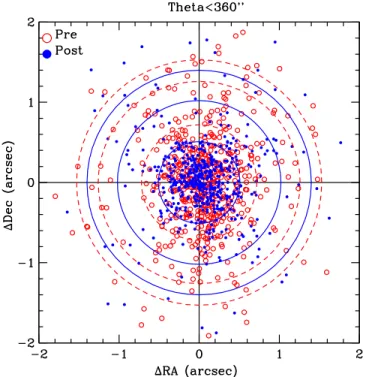
(3) The Astrophysical Journal, 819:62 (18pp), 2016 March 1. Civano et al.. pointings (numbered black points in Figure 1) were used, 11 of which were scheduled as two or more separate observations because of satellite constraints, for a total of 68 pointings. Moreover, the observing roll angle was constrained to be within 70±20 degrees or 250±20. We summarize the main properties of the new Chandra COSMOS-Legacy observations in Table 1. The observations took place in four blocks: 2012 November to 2013 January; 2013 March to July; 2013 October to 2014 January; and 2014 March. The mean net effective exposure time per field was 48.8 ks after all the cleaning and reduction operations (see Section 4). The maximum exposure was 53 ks (observation 15227) while the minimum exposure was 45.2 ks (combined observations 15208 and 15998). The sequence of the observations was designed to start from the N–E top corner tile of C-COSMOS, move toward W, and proceed clockwise around the central C-COSMOS area in such a way that the outer frame of the C-COSMOS survey overlaps with the inner frame of the new Chandra observations. The tiling number and the total area covered is shown in Figure 1. Using this tiling strategy we achieve an approximately uniform combined PSF across the survey. The mean combined PSF width (size at 50% of the encircled energy fraction, EEF, in the 0.5–7 keV band; see Section 5 for details on the PSF maps) weighted on the exposure peaks at around 3″ (see Figure 2). As shown in Figure 2, 80% of the field has a PSF in the range 2″–4″. As a comparison, in a single-pointed survey (regardless of exposure time) the PSF size distribution is flat, and although ∼30% of the field has a PSF <2″ it can reach a substantially larger size (>4″) in 40% of the field.. et al. submitted), we performed source detection on each individual observation to register them to a common optical astrometric frame. This work has been done on the new observations and also on the C-COSMOS outer frame fields and was overlapping with the new data. We generated a list of detected sources using the CIAO wavelet source detection tool WAVDETECT on each single observation binned at 1″ and adopted a false-positive detection probability threshold corresponding to ∼10 spurious sources per field. Of the detected sources (on average 150 sources per field) we considered in each field those with significance >3.5σ and within 360″ from the aim point. In Chandra data the positional accuracy of significant sources is <1″ even at 10′ off-axis and it is energyindependent (K. Glotfelty 2015, private communication). Therefore, choosing sources within 6′ of the aim point provides a sample of sources with a very good centroid estimate (<0 3) for astrometric purposes. Using the CIAO tool reproject_aspect, these sources were then compared with the CFHT MegaCam catalog of i-band-selected sources (McCracken et al. 2012) with optical magnitudes in the range 18–23 AB mag. At least four sources in each field, that are not on the same side of the aim point, are needed to compute meaningful rotational and translation transformations. In our analysis we used on average 12 sources (up to 22 sources per field) with 75% of the fields having more than 10 sources used to perform the reprojection. With the corrected aspect solution we reprocessed the level 1 data using chandra_repro and performed the WAVDETECT detection again to compute the new separation between X-ray and optical positions. The resulting standard deviation on the shift computed from the detected sources within 6′ is 0 36 and 0 51 on the R.A. and decl., respectively. After matching all the X-ray fields to the same astrometric optical frame, 95% of the X-ray sources used for the astrometry correction have a distance to their optical counterpart smaller than 1 4, 10% lower than the value before the correction (1 53). The improvement in the position increases to 20% when considering 90% of the sources (1 26 to 1 02) and 30% when considering a smaller sample of 68% of the sources (from 0 72 to 0 51; see Figure 3). This is consistent with and slightly better than what was found for C-COSMOS (see E09, Figure 6).. 3. DATA PROCESSING The data reduction was performed following the procedures described in E09 for C-COSMOS using standard Chandra CIAO 4.5 tools (Fruscione et al. 2006) and CALDB 4.5.9. We also reprocessed the 49 C-COSMOS observations to use them in concert with the new observations for source detection in the area where the new observations overlap with the old ones and to compute the sensitivity of the whole survey (see the comparison between fluxes in Section 4.1.3). We used the chandra_repro reprocessing script, which automates the CIAO recommended data processing steps and creates new level 2 event files, and applied the VFAINT mode for ACIS background cleaning to all the observations. We then performed the following steps before starting data analysis: astrometric correction and reprocessing of all the observations to a standard frame of reference using the new aspect solution (Section 3.1); mosaic and exposure map creation in three standard Chandra bands (Section 3.2): 0.5–7 keV, 0.5–2 keV and 2–7 keV; background map creation using a two-components model to take into account both the cosmic background contribution and the instrumental one (Section 3.3).. 3.2. Exposure Maps and Data Mosaic Creation We created exposure maps in three bands using the standard CIAO procedure. The spectral model used for the map creation is a single power-law with a slope of Γ=1.433 and Galactic absorption of NH =2.6×1020 cm−2 (Kalberla et al. 2005). Instrument maps generated with MKINSTMAP for each CCD in each observation were used as input files for the MKEXPMAP tool, which computes an exposure map for each CCD separately. These exposure maps were combined in a single exposure map for each observation using DMREGRID with a binning of 2 pixels. Figure 4 shows a composite image of the effective exposure time (in seconds) in the full band for both the new observations (left) and the whole COSMOS-Legacy (right). As can be seen,. 3.1. Astrometric Corrections Even though Chandra data astrometry is accurate to 0 6 (at 90% confidence, see Proposer User Guide32 Chapter 5), to produce a sharp X-ray mosaic and to match the positions of X-ray sources with the optical catalog for which the positional accuracy is ∼0 2 (Capak et al. 2007; Ilbert et al. 2009; Laigle 32. 33. The choice of such a spectral slope is not only because of consistency with E09 and P09, but it is also the slope of the cosmic X-ray background (e.g., Hickox & Markevitch 2006) and therefore well represents a mixed distribution of obscured and unobscured sources at the fluxes covered by COSMOSLegacy.. http://cxc.cfa.harvard.edu/proposer/POG/html/chap5.html#tth_fIg5.5. 3.

(4) The Astrophysical Journal, 819:62 (18pp), 2016 March 1. Civano et al.. Table 1 COSMOS-Legacy Survey (CLS) Observation Summary Fielda. Obs. ID. R.A.. Decl.. Date. Exp. Time (s). Roll (deg). CLS_1. 15207 15590 15591 15208 15598 15209 15600 15604 15210 15211 15605 15212 15606 15213 15214 15215 15216 15217 15218 15219 15220 15221 15222 15223 15224 15225 15226 15227 15228 15229 15230 15231 15232 15649 15233 15234 15653 15235 15236 15237 15655 15238 15239 15240 15241 15242 15243 15244 15245 15246 15247 15248 15249 15250 15251 16544 15252 15253 15254 15255 15256 15257 15258. 150.544451 150.544402 150.544454 150.415643 150.415625 150.295749 150.295747 150.164741 150.164738 150.045569 150.045586 149.913425 149.913418 149.796052 149.751287 149.704144 149.654208 149.627509 149.584767 149.538688 149.614659 149.753949 149.870306 149.999623 150.115609 150.245495 150.411336 150.463753 150.504029 150.551660 150.592692 150.642972 150.690403 150.690409 150.734924 150.616710 150.594589 150.480833 150.364822 150.228563 150.228550 150.114727 149.981160 149.617459 149.593992 149.547344 149.499113 149.547442 149.680897 149.796705 149.953115 150.047419 150.516513 150.566083 150.612991 150.613008 150.660018 150.707972 150.753963 150.661405 150.504801 150.384246 149.497504. 2.499045 2.499094 2.499065 2.543225 2.543213 2.588083 2.588106 2.639752 2.639709 2.682903 2.682879 2.732850 2.732845 2.772968 2.655331 2.525446 2.399733 2.272922 2.145874 2.017596 1.846399 1.801935 1.757718 1.706079 1.664373 1.621716 1.697830 1.829216 1.950647 2.080265 2.199969 2.325853 2.449284 2.449315 2.575875 2.623373 2.629150 2.671101 2.714260 2.765929 2.765907 2.808579 2.858739 2.695912 2.566795 2.443553 2.312060 1.723759 1.673516 1.629086 1.578784 1.537353 1.655025 1.783479 1.904134 1.904121 2.034094 2.162869 2.289683 2.741395 2.795740 2.838987 2.746858. 2012 Nov 25 2012 Nov 23 2012 Nov 25 2012 Dec 07 2012 Dec 08 2012 Dec 03 2012 Dec 05 2012 Dec 10 2012 Dec 16 2012 Dec 13 2012 Dec 15 2012 Dec 21 2012 Dec 23 2013 Jan 01 2013 Jan 03 2013 Jan 07 2013 Jan 16 2013 Mar 23 2013 Mar 22 2013 Mar 30 2013 Apr 04 2013 Apr 10 2013 Apr 04 2013 Apr 17 2013 Apr 19 2013 Apr 05 2013 Jun 21 2013 May 02 2013 Apr 30 2013 May 10 2013 May 08 2013 May 13 2013 May 16 2013 Jun 03 2013 May 21 2013 May 22 2014 Jan 16 2013 Jun 01 2013 Jun 01 2013 Jun 08 2013 Jun 10 2013 Jun 09 2013 Jun 11 2013 Oct 15 2014 Mar 28 2013 Jun 22 2013 Jul 05 2014 Jan 21 2014 Jan 23 2013 Oct 22 2014 Mar 18 2013 Nov 13 2013 Nov 29 2013 Dec 12 2013 Dec 03 2013 Dec 04 2013 Dec 14 2014 Jan 28 2014 Jan 29 2014 Mar 24 2014 Jan 13 2014 Jan 04 2014 Jan 01. 14883 14893 19828 22985 22193 23775 21795 20988 24365 23572 21801 25249 25219 49435 45983 49437 46459 46057 46475 49432 49924 49431 49407 50905 49426 49631 49428 53051 49432 49012 49429 48446 35085 15251 46476 5439 44895 49440 49435 25246 24466 49429 49430 48450 48600 49432 47985 47461 49437 48850 49545 49438 45635 49315 29702 19830 49434 49132 49139 49435 49943 49435 49432. 70.2 70.2 70.2 70.2 70.2 70.2 70.2 70.2 70.2 70.2 70.2 70.2 70.2 62.2 61.75 63.2 56.7 265.2 265.2 261.6 60.1 58.2 60.0 55.2 55.2 59.8 250.2 50.2 50.2 52.2 52.2 51.0 50.6 50.65 50.20 50.20 58.21 48.31 48.23 50.65 50.65 50.65 50.20 77.09 260.21 50.20 50.20 53.21 53.21 75.21 267.21 71.61 70.21 70.21 67.91 67.91 70.21 53.21 53.21 260.21 59.21 61.85 62.27. CLS_2 CLS_3 CLS_4 CLS_5 CLS_6 CLS_7 CLS_8 CLS_9 CLS_10 CLS_11 CLS_12 CLS_13 CLS_14 CLS_15 CLS_16 CLS_17 CLS_18 CLS_19 CLS_20 CLS_21 CLS_22 CLS_23 CLS_24 CLS_25 CLS_26 CLS_27 CLS_28 CLS_29 CLS_30 CLS_31 CLS_32 CLS_33 CLS_34 CLS_35 CLS_36 CLS_37 CLS_38 CLS_39 CLS_40 CLS_41 CLS_42 CLS_43 CLS_44 CLS_45 CLS_46 CLS_47 CLS_48 CLS_49 CLS_50 CLS_51 CLS_52. 4.

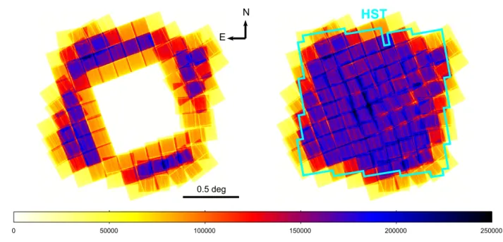
(5) The Astrophysical Journal, 819:62 (18pp), 2016 March 1. Civano et al. Table 1 (Continued). Fielda CLS_53 CLS_54 CLS_55 CLS_56. Obs. ID. R.A.. Decl.. 15259 15260 16562 15261 15262. 149.451159 150.690908 150.690921 150.736977 150.782957. 2.620733 1.740589 1.740576 1.863191 1.992193. Figure 2. Normalized distribution of the combined point-spread function (50% of EEF in 0.5–7 keV) size in arcseconds measured in COSMOS-Legacy (solid histogram) and in a single-pointing survey (dashed line). Red indicates the distribution of the combined PSF (the mean value) for all the detected sources.. Date 2014 2014 2014 2014 2014. Jan Jan Jan Jan Jan. 27 05 25 18 12. Exp. Time (s). Roll (deg). 49435 22793 26736 46474 50236. 53.21 60.21 60.21 59.21 59.21. Figure 3. X-ray to I-band separation (ΔR.A., Δdecl.) in arcseconds for X-ray sources within 6′ from the aim point detected in each single observations before (red open circles) and after ( blue solid circles) the aspect correction. The circles encompass 68%, 90%, and 95% of the sources before (red dashed line) and after (blue solid line) the correction.. the central 1.5 deg2 covers almost the entire HST area and has a uniform depth of 160 ks. The data mosaic image was created in three bands using the HEASoft add images tool which adds together a set of images using sky coordinates. Figure 5 shows the three-colored image that was created by combining the exposure-corrected images in three non-overlapping bands (0.5–2.0 keV, 2.0–4.5 keV, and 4.5–7.0 keV as red, green, and blue, respectively). The combined image was then Gaussian smoothed with a 3 pixel radius. A filter was then applied to isolate the sources from the background level as well as to increase the contrast and color vibrancy of those sources. This process was repeated three times.. The background maps were computed for each observation separately in the full, soft, and hard bands. We ran WAVDETECT with a threshold parameter of sigthresh=10−5 corresponding to ∼100 spurious sources per field (see Section 3.1), which was large enough to also select sources with significant signals only in stacked emission. We then removed these sources from the science images by excising a region corresponding to the source size (using a 3σ value) as computed by the detection tool. We then uniformly distributed the remaining counts and rescaled by the ratio between the whole area of the observation and the area without the removed sources. These files were then used as initial background. We then downloaded “stowed background” data from the Chandra archive.34 Stowed background files are particle-only background files and are obtained when the ACIS detector is out of the focal plane. These files were then rescaled using the procedure described in Hickox & Markevitch (2006): we measured the ratio between the number of counts in our initial background (Cdata) and in the stowed image (Cstow) in the. 3.3. Background Maps Creation The Chandra background consists of two different components: the cosmic X-ray background and a quiescent instrumental background due to interactions between the ACIS-I CCD detectors and high-energy particles. We followed the procedure described in Cappelluti et al. (2013) to create background maps which we used for the selection of reliable sources in our detection procedure and for the computation of the sensitivity curves.. 34. 5. http://cxc.harvard.edu/ciao/threads/acisbackground/.

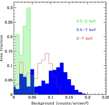
(6) The Astrophysical Journal, 819:62 (18pp), 2016 March 1. Civano et al.. Figure 4. Mosaic of exposure maps for the new observations (left) and for the whole COSMOS-Legacy survey (right) in the full band. The color bar gives the achieved effective exposure in units of seconds. We reached a uniform coverage of ∼160 ks over the full HST area (cyan polygon).. presented by A. Finoguenov et al. (2016, in preparation). To avoid contamination by extended sources we used the XMMCOSMOS catalog of extended sources (Finoguenov et al. 2007; Kettula et al. 2013) and visually inspected all the brightest (LX > 1041 erg s−1 in 0.5–2 keV) ones to check if a point source is detected inside them by Chandra. Puccetti et al. (2009) extensively discussed and compared different source detection techniques and concluded that the best procedure for C-COSMOS was a combination of PWDetect (Damiani et al. 1997) and the Chandra Emldetect (CMLDetect) maximum likelihood algorithm. As shown by P09 using extensive simulations, one of the strongest features of PWDetect is its ability to locate X-ray sources with extreme accuracy (0 02±0 15, P09, Table 1) while CMLDetect is the best tool with which to perform source photometry and derive source significance. The COSMOSLegacy survey shares the same tiling layout, exposure time per field, and roll angle range of C-COSMOS hence we can follow the P09 procedure and use the same significance threshold for source detection. The original version of CMLDetect, called emldetect (Cruddace et al. 1988; Hasinger et al. 1993), is part of the XMM-Newton SAS package and is based on a code originally developed for ROSAT data. CMLDetect has been adapted to run on Chandra data by replacing the XMM-Newton PSF library with the Chandra one (see Krumpe et al. 2015 for another application of CMLDetect). Moreover, this new tool can also work with different PSFs simultaneously. PWDetect was developed to properly treat Chandra data with PSF varying across the field and it is based on the wavelet transform (WT) of the X-ray image. A WT is the convolution of an image with a “generating wavelet” kernel which depends on position and length scale (a free parameter). For this survey and for Chandra data in general, the length scale varies from 0 5 to 16″ in steps of 2 . These steps cover all possible Chandra PSFs (the largest are those at large off-axis angle θi). Both radial and azimuthal PSF variations are accounted for by. energy range 9.5–12 keV. In this band the effective area of Chandra is 0 and consequently all the counts have a nonastrophysical origin. The stowed background was rescaled to our data by Cdata/ Cstow and then subtracted from the initial background to obtain a first version of the cosmic X-ray background. The counts of this map were then renormalized using the exposure maps to create an exposure-corrected cosmic background. Finally we performed a Monte Carlo simulation using the exposure-corrected cosmic X-ray background and the stowed background as input files. We simulated 1000 images for each of the two backgrounds using the IDL routine poidev to obtain a Poissonian realization of each map, and then we obtained our final homogeneous background map adding together the two mean simulated images. To use these maps for sensitivity computations and in our detection algorithm, a Gaussian smoothing (with a scale of 20 pixels) was applied to this final background map using the FTOOL fgauss. The distribution of the computed background (in counts arcsec−2) in the three bands is reported in Figure 6. The overall background count distribution is consistent with the one found in C-COSMOS (see Figure 4 of P09). In the full band the main peak is at around 0.13 counts arcsec−2 and this corresponds to the deepest part of the exposure. In C-COSMOS the deep and shallow areas were roughly the same size and therefore the background distribution had two clear peaks of approximately the same height, while in COSMOS-Legacy the area with higher exposure is three times larger than the shallow area. This is represented in the background distribution as well. The number of background counts is consistent with the expectation for Chandra given the distribution of our exposure times. 4. DATA ANALYSIS: SOURCE DETECTION AND PHOTOMETRY The analysis that follows focuses only on point sources. A parallel effort on the detection of extended sources will be 6.

(7) The Astrophysical Journal, 819:62 (18pp), 2016 March 1. Civano et al.. Figure 5. Three-colored image of the whole COSMOS-Legacy field (0.5–2.0 keV, 2.0–4.5 keV, and 4.5–7.0 keV as red, green, and blue, respectively).. PWDetect which first assumes a Gaussian PSF and then corrects by a PSF shape factor, calibrated with respect to source positions on the CCD. PWDetect works on stacked observations only if coaligned (same aim point and roll angle) as is the case for 11 of our fields which are observations split into multiple parts. Therefore, PWDetect was run on each of our new 56 fields setting the detection limit to 3.8σ and corresponding to a probability of a spurious detection to ;10−4 with the aim of creating a large catalog of detections to be fed to CMLDetect. Also, given that the outer frame of C-COSMOS overlaps with the new survey, we run PWDetect on 20 old fields (fields 1–1 to 1–6, 1–6 to 6–6, 6–6 to 6–1, and last, 6–1 to 1–1 as in Table 3 of E09). For overlapping regions between different pointings we performed. a positional cross-correlation (using a 2″ radius) and if a source was detected in more than one field we chose the position of the source at the smallest θi, i.e., the one with the best PSF. We performed a visual inspection of all the sources having multiple matches within 5″. About 90% of the pairs in the range 2″–5″ were actually false detections, mainly caused by PSF tail detection of bright sources. The positions obtained with PWDetect were then fed as input to CMLDetect to obtain photometric information and significance for each source. We ran CMLDetect allowing the detection only of point-like sources. PWDetect can be used to obtain net counts, rates, and fluxes, but we opted to use CMLDetect because it can work on a mosaic while PWDetect cannot. Moreover, P09 has shown that PWDetect 7.

(8) The Astrophysical Journal, 819:62 (18pp), 2016 March 1. Civano et al. Table 2 Number of Sources with DET_ML>10.8 in at Least one Band, for each Combination of X-Ray Bands Bands. New. C-COSMOS. Legacy. F+S+H F+S F+H F S H Total. 1140 536 448 121 21 7 2273. 1047 (922) 397 (474) 231 (257) 49 (73) 17 (32) 2 (3) 1743 (1761). 2187 933 679 170 38 9 4016. Note. The “New” column includes all the newly detected sources. The columns labeled as “C-COSMOS” include the updated numbers using the information from the new data. The old numbers reported in parentheses are as in Elvis et al. (2009).. P09 performed extensive Monte Carlo simulations for C-COSMOS to both test the detection and photometry strategy as well as to determine the completeness and reliability of the source catalog at the chosen DET_ML threshold. Given that COSMOS-Legacy is the scaled-up version of C-COSMOS (in area and exposure), the same analysis was followed; hence, we infer that the completeness and reliability of the catalog are the same. Therefore, the chosen DET_ML threshold implies a completeness of 87.5% and 68% for sources with at least 12 and 7 full-band counts, of 98.2% and 83% for the soft band, 86% and 67% for the hard band. At this significance level and the same count limits the reliability is ∼99.7% for the three bands.. Figure 6. Distributions of background counts per square arcsecond in the full (solid blue histogram), soft (shaded green histogram), and hard (empty red histogram) bands.. count rates are systematically less accurate than those of CMLDetect (the median ratio between the output detected and input simulated count rates ranges from 86% to 94% for PWDetect versus 97% to 105% for CMLDetect, independently from the energy). CMLDetect performs a simultaneous maximum likelihood PSF fitting for each input candidate source, previously obtained using PWDetect, to all images at each position and working on a mosaic can provide a refined position of the source and count rates. This procedure was run in three bands: full (0.5–7 keV), soft (0.5–2 keV), and hard (2–7 keV). With the goal of not missing close pairs, we run CMLDetect allowing to slightly change the input position provided by PWDetect. The best-fit maximum likelihood parameter in CMLDetect, DET_ML, is related to the Poisson probability that a source candidate is a random fluctuation of the background (Prandom), as follows:. 4.1. Point Source Catalog 4.1.1. Source Numbers. We positionally matched the three single-band CMLDetect output catalogs (including all the sources to DET_ML=6) to one another using a cross-correlation radius of 3″. We first matched the full-band detected source catalog to the soft-band one then the full- with the hard-band catalog and finally the soft and hard-band one. We performed a visual inspection of the whole sample and also made use of the catalog of optical/IR identifications (presented in a companion paper, Marchesi et al. 2016) to solve ambiguous cases. After the visual inspection we found that <1% of the matches were actually fake associations and all related to sources at the outer edges of the survey with rather wide PSFs and therefore with large positional error. Overall the mean (median) separation between detections of the same source in two different bands is 0 43 (0 23) for full to soft and 0 41 (0 23) for full to hard with 90% of the matches within 1″. For soft to hard matches the mean (median) separation is instead 0 73 (0 56), with ∼80% within 1″. The source position is determined in the full band for all the sources detected in the full band; if a source is not detected the full band, the soft band position is used. The hard band position is used for sources detected in the hard band only. In Table 2 we report the total number of new sources for each combination of bands while in Table 4 we report the number of sources detected in each band at the two adopted thresholds (DET_ML>10.8 and 6<DET_ML<10.8). The number of detections with DET_ML>10.8 in at least one of three X-ray bands is 2273. The number of expected spurious. DET_ML = - ln (Prandom) . (1) As a consequence, sources with small values of DET_ML have high values of Prandom and are then likely to be background fluctuations. We chose a threshold significance value of 2×10−5 that corresponds to DET_ML=10.8, i.e., a source needs to have DET_ML>10.8 in at least one of the three bands to be included in the final catalog. This value is the same used in C-COSMOS and represents the best compromise between completeness and reliability as shown by P09 in Figures 11 and 12. Seventy-five percent of the sources detected by PWDetect in a single field with DET_ML>10.8 and fed to CMLDetect were found to be above the threshold in output. To improve the final completeness of the catalog we also search for less significant sources up to about 100 times higher P, which corresponds to a threshold DET_ML=6. Similar to what was done in C-COSMOS, sources with DET_ML in the range 6–10.8 are only considered in this catalog if these have DET_ML>10.8 in another band. Sources with DET_ML<6 are considered undetected.. 8.

(9) The Astrophysical Journal, 819:62 (18pp), 2016 March 1. Civano et al.. Table 3 Number of Spurious Sources with DET_ML>10.8 with at Least 12 and 7 Full-Band Counts, Corresponding to a Reliability of 99.7% for the New Data, the Old C-COSMOS Data (as in P09, Section 5) and the Whole COSMOSLegacy Bands. F S H. New. C-COSMOS. 4.1.2. Source Positional Errors. To compute the positional errors associated with the X-ray centroids given in the catalog ( s 2R.A. + s 2decl. ), we followed the prescription of P09 defining err_pos = rPSF S , where S is the number of net (i.e., background subtracted) source counts in the full band in a circular region of radius rPSF containing 50% of the encircled energy in the observation where the source is at the smallest off-axis angle. The positional errors are generally in very good agreement with those resulting from CMLDetect. In Figure 8 the positional error distribution is presented for all the new sources (black solid line), the old C-COSMOS sources (red dashed line), and the updated C-COSMOS distribution (blue dotted line). The sources plotted in the lowest bin are those with positional error values actually smaller than 0 1 which we set to 0 1, consistent with the work done in P09. These sources with small positional errors are just very bright objects (with ∼240 mean full band counts; see next section). The peak of the new sources distribution is ∼0 6 and 85% of the sources have a positional error <1″ while C-COSMOS source distributions peak at around 0 4. This difference (the somewhat larger positional errors for the sources detected with the new data than for those detected in C-COSMOS) is due to the fact that as shown in Figure 9 the net counts distribution for the sources in the new data peaks at a lower value than for the C-COSMOS sources (therefore giving a smaller denominator in the formula of the positional error).. Legacy. >7. >12. >7. >12. >7. >12. 5 4 3. 5 3 3. 6 4 4. 6 3 3. 12 9 8. 11 7 7. sources with DET_ML>10.8 is reported in each band for two count limits in Table 3. In the area where the new data overlap with the outer C-COSMOS frame, the exposure time is now double the previous mean exposure time (142 ks versus 72 ks) and 385 new sources are detected in addition to the 694 sources already in E09. For the last 694 sources with doubled exposure time, 676 have been detected in the new data as well. The 18 C-COSMOS sources not detected in the new data had DET_ML values in E09 in the three bands close to the threshold (DET_ML<15); moreover, 10 of them were detected only in two out of three bands in E09 and the remaining eight were detected only in one band. In Table 2 we include the number of sources in each combination of bands for the C-COSMOS area including the new data and also in parentheses the number of sources as in E09. The same old and new numbers are included in Table 4. In this paper we provide also an updated catalog of the C-COSMOS sources with larger exposure in the total data. Among the 676 C-COSMOS sources with new data only ∼1.5%, ∼2%, and ∼3% in the full, soft, and hard band, respectively, have a DET_ML value which is below the threshold in the combined data while it was above the 10.8 DET_ML threshold in the C-COSMOS catalog, confirming the reliability of the detection method and the consistency between the analysis performed in E09 and P09 and the one performed here. The actual fraction of sources with DET_ML lower in the combined data set than in C-COSMOS is 14% in the full and 10% in the soft and hard bands. On average, sources with lower DET_ML in the new data set are in an area of the field where the ratio (exp _new - exp _old) exp _old is 40% lower than the average ratio of the sources in the catalog. Therefore, the discrepancy could be explained with source variability. The total number of sources summing the two data sets is reported in the last column of Table 2. Adding the new observations we more than double the sample with respect to C-COSMOS and obtain a catalog of 4016 sources, the largest sample of X-ray sources homogeneously detected and having uniform multiwavelength data (see Section 7 for a discussion and Marchesi et al. 2016). In comparison, other contiguous surveys with similar area in the literature have about 20% fewer sources than COSMOS-Legacy (see 3362 sources in Stripe 82 by LaMassa et al. 2013a, 2013b, 2015; 3293 in X-Bootes by Murray et al. 2005; 2976 in XDEEP2 by Goulding et al. 2012). In Figure 7 we show the signal-to-noise ratio (S/N=count rate/count rate error) as a function of the DET_ML for the new sources with DET_ML>10.8. In excellent agreement with the finding in C-COSMOS, the S/N increases smoothly with increasing DET_ML with a dispersion of a factor of 2 at both low and high DET_ML values.. 4.1.3. Source Counts and Fluxes. The count rates in three bands reported here were obtained with CMLDetect. Vignetting and quantum efficiency were taken into account when measuring the effective exposure time. The count rate error at 68% confidence level was computed CS,90% + (1 + a) ´ B90%. , where CS is using the equation err_rate = 0.9 ´ T the source net count estimated by aperture photometry using an extraction radius including 90% of the EEF for each observation where the source was detected; B is the background count estimated in the same aperture on the background maps used in CMLDetect and corrected with a factor a=0.5 introduced to account for the uncertainties on the background estimation in a given position (see P09); T is the vignetting corrected exposure time. In Figure 9 the net count distributions for the new sources in three bands are compared with those in E09 (C-COSMOS old) and also with the updated counts distribution of C-COSMOS (C-COSMOS new). The total is the sum of the new detections plus the updated C-COSMOS. The median (mean) value of net counts in the whole data set in full, soft, and hard bands is 30, 20, and 22 (80, 60, and 43), respectively, compared to C-COSMOS where we had 33, 22, and 23 (88, 65, and 46). The total number of net counts for the 676 C-COSMOS sources also detected in the new data set is on average 60%–80% larger than the number of counts in C-COSMOS only. As a consequence the updated C-COSMOS count histograms in Figure 9 are all shifted to a higher numbers of counts. While in the full band the peak of the distribution is still around 30 counts we more than double the number of sources with more than 70 full-band counts, for which it is possible to perform individual X-ray spectral analysis from 390 (Lanzuisi et al. 2013) to ∼950 sources in COSMOS-Legacy. The fluxes were obtained from the count rates using the relation F=R×(CF×10−11), where R is the count rate in 9.

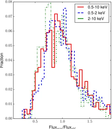
(10) The Astrophysical Journal, 819:62 (18pp), 2016 March 1. Civano et al.. Table 4 Number of Sources Detected in each Band at the two Adopted Thresholds DET_ML  10.8. Band Full (F) Soft (S) Hard (H). 6<DET_ML<10.8. New. C-COSMOS. Legacy. New. C-COSMOS. Legacy. 2146 1538 1325. 1667 (1655) 1382 (1340) 1115 (1017). 3813 2920 2440. 99 159 271. 57 (71) 79 (88) 165 (165). 156 238 436. Note. The columns labeled as C-COSMOS include the updated numbers using the information from the new data. The old numbers are in parentheses as in Elvis et al. (2009).. Figure 9. Source count distributions in three bands: 0.5–7 keV (top), 0.5–2 keV (center), and 2–7 keV (bottom) for COSMOS-Legacy (solid red line), new data only (blue dashed line), C-COSMOS old (green dotted–dashed), and updated (black solid). Sources with an upper limit have not been included.. Figure 7. Signal-to-noise ratio as a function of DETML for sources detected in three bands. The new Chandra sources are plotted as red circles and the C-COSMOS sources as blue ones. We plot only sources with DETML>10.8.. each band and CF is the energy conversion factor computed using the CIAO tool srcflux, assuming a power-law spectrum with slope of Γ=1.4 and a Galactic column density of NH=2.6×1020 cm−2. Due to the fact that the observations have been taken in two different Chandra cycles, i.e., Cycle 8 for C-COSMOS and Cycle 14 for the new data, we used as CF a weighted mean of the factors in the different cycles depending on the exposure time for each source accumulated in each cycle to account for its variation (∼15% between the two cycles). The Cycle 14 (Cycle 835) CFs are 1.71 (1.57), 7.40 (6.34), and 3.06 (3.04) counts erg−1 cm2 for 0.5–10, 0.5–2, and 2–10 bands, respectively. The conversion factors are sensitive to the assumed spectral shape: for Γ=2, there is a change of 40% in the full band CF, ∼5% in the soft band and ∼20% in the hard band. For the 676 C-COSMOS sources detected in the new data as well, we computed new total X-ray fluxes. In Figure 10 the normalized distribution of ratios between total and old fluxes are plotted for the three bands. From Gaussian fitting of the distributions we find centroids at (Fnew /Fold)=1.06, 1.11, 0.99, and standard deviations of ∼0.50, ∼0.55, and ∼0.40 in 35 The CF used for C-COSMOS and reported in E09 and P09 (computed using the online tool PIMMS) slightly differ from the one used here because the latter are now computed with the most updated response matrix. The difference is ∼15% and it reflects on the final fluxes for all C-COSMOS sources.. Figure 8. Positional error distribution for the new COSMOS-Legacy data (black solid line), the original C-COSMOS (red dashed line), and the updated C-COSMOS (blue dotted line).. 10.

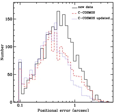
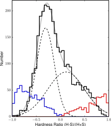
(11) The Astrophysical Journal, 819:62 (18pp), 2016 March 1. Civano et al.. Figure 11. Flux distributions for sources detected in 0.5–10 keV (top), 0.5–2 keV (center), and 2–10 keV (bottom) bands for COSMOS-Legacy (solid red line), new data only (solid blue line), C-COSMOS updated (black dotted line) and XMM-COSMOS (cyan dashed line) sources. We also include the CDFS 4 Ms source flux distribution (orange line) and the Stripe 82 sources (green line). Sources with an upper limit have not been included.. Figure 10. Normalized distributions of ratios between new and old fluxes of the 676 sources detected in C-COSMOS and also in the new data at DET_ML>10.8. Sources with an upper limit have not been included.. full, soft, and hard bands, respectively, showing a good agreement between old and new fluxes. The distributions show wings to both negative and positive values. Malmquist bias is most likely responsible for the negative wing while variability for the positive one. The distributions of X-ray fluxes for the whole Chandra COSMOS-Legacy survey in the full, soft, and hard bands is shown in Figure 11 where it is also compared with C-COSMOS (the new version with just the updated fluxes, given the excellent agreement) and XMM-COSMOS. The new survey is about ∼2.5 times deeper than XMM-COSMOS in the 0.5–2 keV band and ∼2 times in the 2–10 keV band and more than doubles the number of C-COSMOS sources in the same flux range. In the same figure we compare our data with the 4 Ms CDFS (Xue et al. 2011) and the large area Stripe 82 survey (LaMassa et al. 2013a, 2013b) source flux distributions, respectively to the left and to the right of COSMOS-Legacy flux distribution. The combination of the three surveys (the deepest, the intermediate, and among the widest; see also Section 7) allows to cover more than four orders of magnitude in flux. Upper limits (90% confidence level) on net counts, count rates, and fluxes are given for all sources found in one band but not detected in another band. The upper limits were computed with the same procedure adopted for C-COSMOS and largely described in P09 to which we refer for a complete description.. hard band and S is those obtained in the soft band. Given the low number of counts for most of the sources (see Figure 9), we used BEHR (Bayesian Estimation of HRs, Park et al. 2006) which is particularly effective in the low-count regime, not needing a detection in both bands to work. We extracted aperture photometry counts from each observation where the source was detected using the PSF radius at EEF=0.9. We also extracted the background counts from the same observations using an annulus with rmin = rPSF + 8 pixels and rmax = rPSF + 40 pixels, where rPSF is the PSF radius at EEF=0.95 (in pixels). In the background extraction we excluded the contamination by other nearby detected sources using an exclusion radius equal to rPSF. Total counts, background counts, and the ratio between the sum of background areas and the sum of source areas, both in soft and hard bands, were then fed as input parameters to BEHR. For most sources (>3000) BEHR finds a detection on the HR and for 989 sources an upper or lower limit (616 and 371 sources, respectively). The typical error on the HR is ∼0.2. In Figure 12 we plot the distribution of the HRs for the measured values (black solid line), for the lower limits (red solid line) and the upper limits (blue solid line). The mean (median) HR value is −0.09 (−0.17) for the measured values and it moves to lower values when including upper and lower limits (−0.11 and −0.19 for the mean and the median, respectively). A Gaussian fit returns a peak at −0.20 with a 1σ dispersion of 0.32; however, a single Gaussian is not clearly a best representation of the HR distribution. A double Gaussian fit returns a peak at −0.31 and one at 0.12 with a 1σ dispersion of 0.18 and 0.38, respectively. HR is not a fully reliable measurement of obscuration because of the complexity of the spectral shape, the large error. 4.1.4. Hardness Ratio (HR) Analysis. To provide a rough estimate of the X-ray spectral shape of the sources, in particular of the intrinsic obscuration (see Marchesi et al. 2016), for all the sources in the catalog including the C-COSMOS sources we computed the hardness H-S ratio defined as HR= H + S , where H is the net count in the 11.

(12) The Astrophysical Journal, 819:62 (18pp), 2016 March 1. Civano et al. Table 5 Data Fields in the Catalog No.. Figure 12. HR distributions for the whole sample (black solid line), upper limits (blue solid line) and lower limits (red solid line). The dotted line is the sum of the double Gaussian fitting. The dashed lines are the two Gaussian resulting from the fitting.. bars due to low counts statistic, and the redshift dependency (see Marchesi et al. 2016); however, it is possible to roughly assume an HR value to divide the sources in obscured and unobscured. We use here HR=–0.2 which has been shown to be a fair value to separate sources with column densities above and below 1022 cm−2 (Civano et al. 2012; Lanzuisi et al. 2013) +17 at all redshifts. A total of 1993 sources, 5016 % of the entire sample (errors have been computed using HR 1σ errors) are therefore classified as obscured. Tentatively the double Gaussian fit of the HR distribution could also be interpreted as to be due from two populations of sources, the obscured population peaking at positive HRs and the unobscured population peaking at negative HR. The broad dispersion of the Gaussian peaking at positive HR could be due to high redshift-obscured sources whose HR would be negative even if obscured. A more detailed analysis on the obscured AGN fraction is presented in Marchesi et al. (2016).. Chandra source name Chandra Right Ascension (J2000, hms) Chandra Declination (J2000, dms) Positional error (arcsec). 5. DET_ML_F. 6 7 8 9 10 11 12 13. rate_F rate_F_err flux_F flux_F_err snr_F exptime_F cts_ap_F cts_ap_F_err. maximum likelihood detection value in 0.5–7 keV band 0.5–7 keV count rate (counts s−1) 0.5–7 keV count rate error (counts s−1) 0.5–10 keV flux (erg cm−2 s−1) 0.5–10 keV flux error (erg cm−2 s−1) 0.5–7 keV S/N 0.5–7 keV exposure time (ks) 0.5–7 aperture photometry counts (counts) 0.5–7 aperture photometry counts error (counts). 14. DET_ML_S. 15 16 17 18 19 20 21 22. rate_S rate_S_err flux_S flux_S_err snr_S exptime_S cts_ap_S cts_ap_S_err. maximum likelihood detection value in 0.5–2 keV band 0.5–2 keV count rate (counts s−1) 0.5–2 keV count rate error (counts s−1) 0.5–2 keV flux (erg cm−2 s−1) 0.5–2 keV flux error (erg cm−2 s−1) 0.5–2 keV S/N 0.5–2 keV exposure time (ks) 0.5–2 aperture photometry counts (counts) 0.5–2 aperture photometry counts error (counts). 23 24 25 26 27 28 29 30 31. DET_ML_H rate_H rate_H_err flux_H flux_H_err snr_H exptime_H cts_ap_H cts_ap_H_err. maximum likelihood detection value in 2–7 keV band 2–7 keV count rate (counts s−1) 2–7 keV count rate error (counts s−1) 2–10 keV flux (erg cm−2 s−1) 2–10 keV flux error (erg cm−2 s−1) 2–7 keV S/N 2–7 keV exposure time (ks) 2–7 aperture photometry counts (counts) 2–7 aperture photometry counts error (counts). 32 33 34. hr hr_lo_lim hr_up_lim. Hardness ratio Hardness ratio 90% lower limit Hardness ratio 90% upper limit. 4.2. Matching with XMM-COSMOS Catalog We matched the COSMOS-Legacy sources with those in XMM-COSMOS (Cappelluti et al. 2009). There are 1714 secure XMM-COSMOS sources with at least one counterpart in COSMOS-Legacy, 824 of which have at least one counterpart in the new data. There are 46 XMM-COSMOS sources outside the area covered by COSMOS-Legacy (see Figure 1) and 126 with no Chandra counterparts. In summary, 93% of the XMM-COSMOS sources within the COSMOS-Legacy area have at least one Chandra counterpart. The 126 sources with no Chandra counterparts can be divided into three groups: the 25 sources (20%) with Chandra exposure lt40 ks; the 60 sources (48%; 13 of these sources have also Chandra exposure <40 ks) with XMM-COSMOS DET_ML<15 in all of the three bands (0.5–2 keV, 2–8 keV, 4.5–8 keV); and last, the 54 sources with XMMCOSMOS DET_ML>15 in at least one band and Chandra exposure >40 ks. For the first group the low exposure time could be the reason for the non-detection while for the second. The catalog released with this paper contains all the measurements discussed above. In Table 5 we show the columns of the catalog of the new 2273 sources (named as “lid” in column 1) combined with the updated C-COSMOS catalog of 1743 sources (named as “cid” in column 1). The catalog will also be stored on the COSMOS website at the COSMOSLegacy project page.36 Data products including exposure and events mosaics are available in the dedicated page37 at the same website. 37. Note. Name R.A. Decl. pos_err. (This table is available in its entirety in machine-readable form.). 4.1.5. Source Catalog. 36. Field. 1 2 3 4. http://irsa.ipac.caltech.edu/data/COSMOS/tables/chandra/ http://irsa.ipac.caltech.edu/data/COSMOS/images/chandra/. 12.

(13) The Astrophysical Journal, 819:62 (18pp), 2016 March 1. Civano et al.. group the non-detection in Chandra can be explained with a flux fluctuation within the flux uncertainty. We visually inspected the sources in the last group and we found that seven of them are located inside a bright cluster and therefore have not been resolved into point sources by our analysis. For the remaining 47 sources the Chandra signal is weak or negligible and therefore these sources could be candidate variable AGN. In particular, XMM-ID 30748 has DET_ML 20 times larger than the detection threshold in XMM-COSMOS; this source was detected only in the 0.5–2 keV band, with a flux of F=2.7×10−15 erg s−1 cm−2 and a photometric redshift of z=2.71. Despite being interesting and worth further analysis on the variability, this is beyond the scope of this paper. There are 58 XMM-COSMOS sources that have been resolved by the smaller Chandra PSF into two distinct sources using a maximum radius of 10″ for the match. Two XMMCOSMOS sources have been resolved into three Chandra sources using a maximum radius of 10″. As a comparison, 25 XMM-COSMOS sources (Brusa et al. 2010) were resolved into two separate C-COSMOS sources. More details on the optical counterparts of the XMM-COSMOS sources resolved in two Chandra ones are given in Marchesi et al. (2016). There is a good agreement between XMM-COSMOS and Chandra fluxes. We rescaled the Chandra COSMOS-Legacy fluxes using the same slope used for XMM-COSMOS (Γ=2 in soft band and Γ=1.7 in hard band) and found that the median value of the ratio fluxXMM flux Chandra is 1.13 in soft band and 1.22 in hard band.. Figure 13. Area-flux curve for COSMOS-Legacy (red solid line) in 2–10 keV (top), 0.5–2 keV (center) and 0.5–10 keV (bottom) bands. The coverage of C-COSMOS (black solid line) and XMM-COSMOS in the 0.5–2 keV and 2–10 keV bands (Cappelluti et al. 2009; blue dashed line) are shown for comparison.. background fluctuations, assuming the same probability for spurious sources (i.e., DET_ML threshold) used in the C-COSMOS and COSMOS-Legacy catalogs for the Poisson statistics, i.e., 2×10−5. We used the relation. 5. SKY COVERAGE AND SURVEY SENSITIVITY The sky coverage of a survey is the area covered as a function of the flux limit. We computed it in three bands (0.5–10, 0.5–2, and 2–10 keV) using the exposure and background maps (see Sections 3.2 and 3.3) produced for the source detection and assuming a power-law spectrum with Γ=1.4 and Galactic NH=2.6×1020 cm−2. X-ray observations have a flux limit that changes over the field of view because the Chandra PSF changes in both size and shape as a function of the distance from the aim point and because the effective area is vignetted. In this survey where the total coverage is obtained using multiple overlapping pointings, every source was observed in up to six different positions on the detector which resulted in a quite uniform average PSF (Figure 2). The procedure we used to compute COSMOS-Legacy survey sky coverage is closely similar to that used by P09 for CCOSMOS but makes use of a PSF map for each observation instead of an analytical form of the PSF as function of the offaxis angle. This is a more time-consuming approach but one that returns a more detailed sensitivity map that can be valuable in other studies (e.g., clustering analysis and correlation functions) or simply for source photometry (Section 4.1.4). For each observation we made use of the CIAO tools mkpsfmap and dmimgadapt to create a background map convolved with the PSF map in such a way that at each position of the map the count value corresponds to the number of counts in an aperture corresponding to 50% of the EEF at that position. For each position of the entire mosaic (applying a binning of 8 pixels for computing time purposes) we computed the minimum number of counts Cmin needed to exceed the. P Poisson = e-B. ¥. Bk = 2 ´ 10-5, ! k k = C min. å. (2 ). where B is the total background count computed at each position of the grid, by summing the background counts in each observation covering that given position. Equation (2) is solved iteratively to find Cmin; then the count rate limit, Rlim is obtained using Rlim =. Cmin - B , fpsf ´ Texp. (3 ). where Texp is the total vignetting corrected exposure time at each position on the grid, while fpsf is the encircled count fraction of the PSF. In C-COSMOS this value was tuned to reproduce the simulation results and then it was fixed to fpsf=0.5. However, any number in the range 0.5–0.9 produced similar results with variations of the order of few percent in the resulting sensitivity. Finally we converted the count rate limit Rlim into the flux limit using the same conversion factors used for the sources in the catalog based on the position (see Section 4.1.3). We also computed the sensitivity for only the C-COSMOS area with the same method and obtained the same sensitivity as published in E09 and P09. The sky coverage of the Chandra COSMOS-Legacy survey in the three energy bands is shown in Figure 13. We compare our results with those of C-COSMOS (black solid lines) and XMM-COSMOS (blue dashed lines). The new survey covers a similar area to XMM-COSMOS and almost three times the area 13.

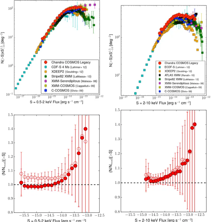
(14) The Astrophysical Journal, 819:62 (18pp), 2016 March 1. Civano et al.. −15. of C-COSMOS at faint fluxes (e.g., ∼5×10 erg cm-2 s-1 in the soft band) and ∼2 times at bright fluxes (e.g., >10−15 erg cm-2 s-1 in the soft band). We have verified that the limits at 20% (50%) completeness for the Legacy catalog are consistent with those computed and reported in Table 2 of P09 and assuming the changes in CF used here and explained in Section 4.1.3 of 1.5 (1.9)×10−15, 3.9 (4.9)×10−16 and 2.5 (3.1)×10−15 erg cm-2 s-1 in the F, S, and H bands. At this limit, COSMOS-Legacy increases by a factor of 3 the area covered with respect to C-COSMOS.. COSMOS-Legacy logN–logS covers 3 and 2.5 orders of magnitude in flux in the soft and hard band, respectively, with 2%–8% errors at fluxes <1–3×10−14 erg cm-2 s-1, respectively. The excellent statistics allow considerable reduction in the uncertainties (20%–30%) in the number counts also at bright fluxes which are now ;40% smaller than in C-COSMOS. In the soft band there is an excellent agreement between our survey and previous works below S ~ 10-14 erg cm-2 s-1. At brighter fluxes instead the uncertainties are larger due to the low number of detections (65 sources in COSMOS-Legacy). A larger spread is observed when comparing results from different surveys due to the fact that bright sources can be properly sampled only with extremely large areas (>5–10 deg2). In the hard band instead, COSMOS-Legacy number counts agree with other surveys at faint fluxes while at the bright end (i.e., S > 2×10−14 erg cm-2 s-1) the COSMOSLegacy counts are in the upper envelope of the spread. We also compare our results with predictions of two different phenomenological models, Gilli et al. (2007) and Treister et al. (2009), assuming column densities in the interval NH= 1020–26 cm−2 and redshift z=0–6. In Figure 14 (bottom panels) we show the ratio of COSMOS-Legacy number counts to both models in the soft and hard bands (left and right). At the faint end of the soft band, i.e., up to fluxes ∼10−14 erg cm-2 s-1, our results are in agreement with the Gilli et al. (2007, solid points) model prediction within 1%–5% while the Treister et al. (2009, open points) model (open points) slightly underpredictions the counts by 5%–10% in the same flux range. At bright fluxes where the sample is limited by the statistics the differences between models and data becomes larger, even exceeding 10%. In the hard band both models reproduce well the observed data within 5% below >2×10−14 erg cm-2 s-1 and the difference becomes more pronounced at bright fluxes (>10% at fluxes >5×10−14 erg cm-2 s-1). The Gilli et al. (2007) and Treister et al. (2009) models are based on different assumptions on the fraction of obscured sources and on the assumed luminosity and redshift dependences. Therefore, their differences are more marked when considering obscured and unobscured sources separately. We used the HR as defined in Section 4.1.4 to divide the sample using HR>−0.2 for obscured sources and HR<−0.2 for unobscured sources. In the soft (hard) band there are 1057 (1332) obscured sources and 1701 (911) unobscured ones. In Figure 15 we present the number counts in the soft and hard bands (left and right) for both obscured (red) and unobscured (blue) sources. A clear difference is observed in the number counts of obscured and unobscured in the soft band where we observe a ratio of up to ∼10 at bright fluxes while it almost disappears in the hard band, where the ratio is very small at all fluxes. This implies that the difference must be dictated by obscuration effects. The models from Gilli et al. (2007, solid lines) and Treister et al. (2009, dashed lines), assuming column densities above and below 1022 cm−2 (red and blue, respectively), are plotted in the same Figure. In the soft band both predictions of the number of unobscured sources are in agreement within 5% with our data up to fluxes of ∼3×10−14 erg cm-2 s-1 while the difference becomes larger for obscured sources (>10%–20%) with both models overpredicting the number of sources at all fluxes. In this last case the Treister et al. (2009) model predictions are generally worse than those of the Gilli et al. (2007) model by 5%–10%. In the hard band instead,. 6. NUMBER COUNTS The logN–logS relation, i.e., the number of sources N(>S) per square degree detected at fluxes brighter than a given flux S (erg s−1 cm−2), provides a first estimate of source space density as a function of flux and therefore information on the cosmic population to compare with different models of population synthesis. Given that multiple logN–logS curves have been published in the literature, it is also a standard check to validate the many calibration steps used to produce a catalog of X-ray point-like sources. We constructed the logN–logS curve for COSMOS-Legacy in both the 0.5–2 keV and 2–10 keV bands. Following P09 we included only sources with DET_ML>10.8 and we applied a cut in S/N (>2 and >2.5 in soft and hard) to limit the Eddington bias effect, which could have a significant (up to 30%–50%) contribution at the lowest fluxes. This choice avoids sources with large statistical uncertainties on their fluxes and limits the errors due to the sky coverage uncertainties at the faint end. With the adopted thresholds in S/N the agreement measured in P09 between simulations input and output logN– logS is better than 5%. The procedure used by P09 is consistent with the one applied by Luo et al. (2008) on Chandra Deep Field South data. The number of sources not included because of the S/N cut is ∼1% in the soft and ∼5% in the hard band. The adopted S/Ns imply the following flux limits: 2.7× 10−16 erg s−1 cm−2 in the 0.5–2 keV band and 1.8× 10−15 erg s−1 cm−2 in the 2–10 keV band. These are the same flux limits of C-COSMOS, which is expected given that the new observations have the same maximum exposure. The final number of sources used here for the number counts with the above constraints are 2758 in the soft band (1309 from C-COSMOS and 1449 from the new sample) and 2243 in the hard band38 (1056 from C-COSMOS and 1187 from the new sample). We show the results obtained with these source selections in Figure 14. In the top panels the normalized Euclidean curves, i.e., with N(>S) multiplied by S1.5, are presented in order to enhance the differences between different surveys. In the same figure we include the C-COSMOS (E09) and XMM-COSMOS points (Cappelluti et al. 2009). We also compare our logN–logS relationships with those from previous X-ray surveys, spanning from wide (Stripe 82 XMM: LaMassa et al. 2013a; 2XMMi: Mateos et al. 2008), to moderate (XDEEP2: Goulding et al. 2012) to small areas (4 Ms CDFS: Lehmer et al. 2012). As XDEEP2 and CDFS define their hard band in a slightly different energy range we converted their energy to 2–10 keV to perform an adequate comparison. 38. We also applied a cut in exposure time at 40 ks in the hard band to limit sources (65 in total) at the edges of the field with high background level.. 14.

(15) The Astrophysical Journal, 819:62 (18pp), 2016 March 1. Civano et al.. Figure 14. Euclidean normalized logN–logS curves in 0.5–2 keV (top left) and 2–10 keV (top right) bands. The COSMOS-Legacy curve for all sources with DET_ML>10.8 and S/N>S/Nlim is plotted in red circles. Results from previous works are plotted (see label in the plot). The ratio of COSMOS-Legacy number counts to Gilli et al. (2007, red solid circles) and Treister et al. (2009; red empty circles) models are plotted in the soft and hard bands (bottom left and bottom right). The source number counts are multiplied by (S 1014)1.5 to highlight the deviations from the Euclidean behavior.. discussion on discrepancies between data and population synthesis models).. model predictions are in general excellent agreement with our data (differences <5% up to fluxes of 5×10−14 erg cm-2 s-1) for both samples above and below HR=–0.2. Overall these discrepancies between data and models are totally expected given that, for example, a different spectral model could change source fluxes and sky coverage, and that the spectral parameters in the Gilli et al. and Treister et al. models are different from those used in this work. Therefore, despite all the underlying assumptions the differences between observed number counts and phenomenological models are remarkably small (2%–5%; see also LaMassa et al. 2013b for a. 7. SUMMARY AND CONCLUSIONS In this paper we presented COSMOS-Legacy, a 2.2 deg2 Chandra survey of the COSMOS field. We employed a total of 4.6 Ms of exposure time including 1.8 Ms already published by E09 plus 2.8 Ms obtained as an X-ray Visionary Project during Chandra Cycle 14. The new data comprise 56 overlapping observations which, added to the 36 C-COSMOS 15.

(16) The Astrophysical Journal, 819:62 (18pp), 2016 March 1. Civano et al.. Figure 15. Number counts in soft (top left) and hard (top right) bands for sources with HR>−0.2 (red squares) and <−0.2 (blue circles) plotted with the Gilli et al. (solid lines) and Treister et al. (dashed lines) models with two different column density ranges >1022 cm−2 in red and <1022 cm−2 in blue. The ratio of COSMOS-Legacy number counts to Gilli et al. (2007; solid) and Treister et al. (2009; empty) models are plotted in the soft and hard bands (bottom left and bottom right).. pointings, yield a relatively uniform coverage of ∼160 ks over the whole Hubble-covered area. By construction the survey flux limit is the same as C-COSMOS and computed in three bands using the same approach of P09. We followed the same procedure used and tested by P09 combining standard CIAO tools for the data reduction and PWDetect and CMLDetect for the data analysis, including. the source detection and photometry. We also performed aperture photometry for consistency with the E09 and P09 analysis. The analysis was performed on the new Chandra data and also on the outer C-COSMOS frame, overlapping with the new observations. Given that the survey properties (exposure, roll angle, and background counts) are consistent with C-COSMOS ones, we used the same probability threshold 16.