A metabolic view of amphibian local community structure: the role of activation energy

Texto completo

(1)ECOGRAPHY Research A metabolic view of amphibian local community structure: the role of activation energy Andrés Canavero, Matías Arim, Fernanda Pérez, Fabián M. Jaksic and Pablo A. Marquet. A. Canavero ([email protected]) and F. M. Jaksic, Center of Applied Ecology and Sustainability (CAPES), Depto de Ecología, Pontificia Univ. Católica de Chile, Santiago, Chile. AC also at: Centro Univ. de Rivera, Univ. de la República, Rivera, Uruguay. – M. Arim and AC, Depto de Ecología y Gestión Ambiental, Centro Univ. Regional Este, Univ. de la República, Maldonado, Uruguay (CURE). MA also at: Facultad de Ciencias, Univ. de la República Uruguay, Montevideo, Uruguay. – F. Pérez, P. A. Marquet, AC and FMJ, Depto de Ecología, Facultad de Ciencias Biológicas, Pontificia Univ. Católica de Chile, Santiago de Chile, Chile. PAM also at: Inst. de Ecología y Biodiversidad (IEB), Santiago, Chile, and The Santa Fe Inst., Santa Fe, NM, USA.. Ecography 41: 388–400, 2018. doi: 10.1111/ecog.02336 Subject Editor: Alison Boyer Editor-in-Chief: Miguel Araújo Accepted 25 January 2017. In the context of the metabolic theory of ecology (MTE), the activation energy (E) reflects the temperature dependence of metabolism and organism performance in different activities, such as calling behavior. In this contribution we test the role of temperature in affecting local amphibian community structure, particularly the number of species engaged in calling behavior across a temperature gradient. Toward this aim, we compiled phenological calling activity for 52 Neotropical anuran communities. For each community we estimated the activation energy of calling behavior (E), finding values significantly higher than previous reports. A wide range of methodological issues with the potential to produce overestimated E-values were shown to have no significant effect on reported E-values, supporting a biological interpretation of their high values and of geographic trends. Further, a path analysis related variation in E among communities with communities’ phylogenetic structure, local environmental conditions, richness, and seasonality. The decrease of activation energy at higher latitudes and less productive environments suggests that amphibians’ activity could become more dependent of internal individuals’ resources once external sources are reduced. The increase in phylogenetic attraction with latitude points to a rise in the role of niche conservatism and community filtering operating over conserved traits. Finally, flexibility in activation energy related to amphibians’ calling could be an important and poorly recognized determinant of their thermal dependence. The temporal structuring of amphians’ communities was related here with the interplay between ecological and evolutionary processes operating at different scales. Our results support the view of activation energy as an important parameter of biodiversity organization, which unravels the effects of ecological and evolutionary processes on biodiversity structure and function.. Introduction One of the major challenges of the metabolic theory of ecology (MTE) is to provide understanding of local community patterns (Marquet et al. 2004a, Tilman et al. 2004). Indeed, although metabolic approaches have been used to understand local ––––––––––––––––––––––––––––––––––––––––. www.ecography.org 388. © 2017 The Authors. Ecography © 2017 Nordic Society Oikos.

(2) community patterns associated with size distributions and density scaling relationships (Brown and Maurer 1986, Marquet et al. 1990, 2004a, Marquet and Taper 1998, Enquist et al. 2009) the fundamental questions of the regulation of species richness, distribution of abundance, and coexistence still remain unresolved (Storch 2012, Brown 2014). One of the fundamental parameters of MTE is the activation energy (E) of metabolism (BT) that expresses the temperature dependence of metabolic rates BT ≈ exp(E/kT), where k is Boltzmann’s constant (8.62  105eV K1, Gillooly et al. 2001) and T is temperature in degrees Kelvin. Using MTE’s canonical equation it has been possible to link changes in environmental temperature with a variety of biologically important processes such as metabolism (Gillooly et al. 2001), mutation rate (Gillooly et al. 2005, 2007, Allen and Gillooly 2006), speciation rate (Allen and Gillooly 2006), species lifetime (Munch and Salinas 2009), and species richness (Allen et al. 2002). Empirical evidence suggests that the activation energy (E) could capture relevant information about the energetic relationship between organisms and their environment (Gillooly et al. 2001, Brown et al. 2004) by making explicit the temperature dependence of organism performance, constrained by their physiology and environment (Stegen et al. 2009, Dell et al. 2011, 2014). In this sense, the analysis of changes in E along natural gradients, as well as across populations and species, could provide novel insights about the determinants of biodiversity structure and function, and its dependence on ambient temperature (Stegen et al. 2009). Indeed, the recently reported variation in E among higher taxa (Caruso et al. 2010, Ehnes et al. 2011) suggests that a species’ evolutionary history could affect how sensitive a species is to environmental temperature variation. A main component of community structure closely related with ambient temperature is the seasonal variation in the number of species that are observed performing some behavior – i.e. phenology. Organisms have evolved vital activities coupled to specific times of year (Emerson et al. 2008). Specifically, phenologies were proposed to originate for seasonal resource tracking, predator avoidance, pollination success, physiological constraints, and/or temporal partitioning of resources (Morin 1999, Sandvik et al. 2002, Kronfeld-Schor and Dayan 2003, Bradshaw and Holzapfel 2007). The recognition of the roles of phenology on ecosystem diversity and functioning, as well as the limitations of ecological theory to account for observed patterns, has positioned its study as a frontier topic in the context of global change (Forrest and Miller-Rushing 2010, Jenouvrier and Visser 2011, Pau et al. 2011, Steen et al. 2013, Scheffers et al. 2016). The phenological trends in anuran calling activity have been thoroughly studied for over half a century (Blair 1961, Inger 1969, Crump 1974) and as expected for ectotherms, environmental temperature is considered as one of the main drivers of anuran phenologies (Bradshaw and Holzapfel 2007, Steen et al. 2013). In consequence, different authors have explored correlation between the mean monthly ambient temperature and the number of species engaged in calling. activities (Saenz et al. 2006, Boquimpani-Freitas et al. 2007, Both et al. 2008, Canavero et al. 2008). The mating call of anurans is an energetically costly behavior whose frequency, power, and duration conform to predictions of MTE (Wells 2007, Gillooly and Ophir 2010, Ophir et al. 2010, Ziegler et al. 2016). Thus, we considered anurans as an appropriate group to obtain insights on this community-level phenological phenomenon through the novel perspective provided by the MTE (Brown et al. 2004). In this article, we compiled information on the phenological calling activity of Neotropical anuran local communities. For each one we estimated the activation energy of calling behavior E – the thermal dependency of the total number of species calling within each local community – from a metabolic model. Then we analyzed the relationship between the activation energy E connecting the number of amphibian species that were calling in each community with environmental gradients related to available energy (e.g. latitude, NDVI, PET), and the phylogenetic similarity of the species composing the local communities. We found relatively high activation energies, which were related with communities’ phylogenetic structure, local environmental conditions, richness, and seasonality. The decrease of activation energy at higher latitudes and less productive environments suggests that amphibians’ activity could become more dependent of internal individuals’ resources once external sources are reduced. Further, the increase in phylogenetic attraction with latitude points to a rise in the role of niche conservatism and community filtering operating over conserved traits.. Material and methods We compiled published data on phenological activity patterns for 52 Neotropical anuran communities. Each phenology involves the number and identity of species calling per month. This compilation includes 361 species from 50 genera, with local community richness ranging from 9 to 39 species, periods of activity lasting between 8 and 24 months, along a latitudinal gradient varying between 7° and 34°S (Fig. 1 and Table 1). The methodologies and scales used to assess the phenological structure of each community were similar: surveys of one to five nights per month recording the presence of anuran species based on their calling behavior (Heyer et al. 1994). A sinusoidal function was fitted to each of the 52 communities: Sa  Smean  Samp sin [2 p (month  c)/12]; where Sa is number of species that call in a particular month (Canavero et al. 2008, 2009). We retain the parameter Samp, which estimates the amplitude of the temporal variation in richness and is used here for the analysis of geographic trends in anurans phenologies. For each community, we obtained information about environmental productivity (NDVI, normalized difference vegetation index), potential evapotranspiration (PET), coefficient of variation in annual precipitation (PCV), annual precipitation (Rain), coefficient of variation in mean monthly temperature (TCV), annual mean temperature. 389.

(3) Figure 1. Geographic locations of the 52 Neotropical data series.. (Tamean), maximum temperature of hottest month (Tmax), and minimum temperature of coldest month (Tmin) from Hijmans et al. (2005) and Rangel et al. (2006). The analysis of observed activation energies E comprises three stages. First, the global information about E values was assessed with a mixed effects model in which the source community was modeled as a random effect. Second, local E values were estimated and the distribution of E values was compared with those calculated by recent reviews for other ecological rates. Third, local variation in activation energy among communities was related with communities’ phylogenetic composition, and biotic and abiotic conditions. Global trend in activation energy. Three linear mixed effects models were fitted by restricted maximum likelihood estimation (REML) with 717 observations (number of species that call in a specific month) in 52 groups (communities) (Zuur et al. 2009). These three linear models included as an independent variable the reciprocal temperature in Kelvin multiplied by Boltzmann’s constant (k), and as dependent variables the natural logarithm of the number of calling species per month (for more details of the models and fitting, see below). Models included community identity as a random effect, considering a random intercept, a random intercept and slope. Models were ranked on the basis of their Akaike’s information criterion values (AIC) (Zuur et al. 2009). Model performances were contrasted with. 390. the AIC and differences in AIC values greater than 2.0 were deemed significant (Hilborn and Mangel 1997, Richards 2005). All linear mixed effects models were done using the nlme package in R ver. 2.15.2 (Pinheiro et al. 2013). Estimating local community activation energy. The estimation of activation energy could be affected by several methodological problems, which could bias our comparison against previously reported values of E. With this in mind we considered several sources of bias on our estimates of E, including: 1) the effect of local richness and the impact of working with absolute or relative richness (Supplementary material Appendix 1); 2) the effect of the range of temperatures evaluated; 3) the fit of nonlinear model (i.e. untransformed) versus log-transformed, log (S  c) local community richness data; 4) the impact of the value of c used in the log-transformation; and 5) the potential impact of autocorrelation in residuals. The putative effect of local community richness on the estimation of activation energy was evaluated by a mathematical argument (Supplementary material Appendix 1). We found that species richness only affects the intercept estimation of the metabolic model and has no effects on the estimation of the activation energy (E). An additional point of concern is the potential increase in the uncertainty associated with the estimation of E when the range of temperatures is narrow. This point was evaluated by exploring.

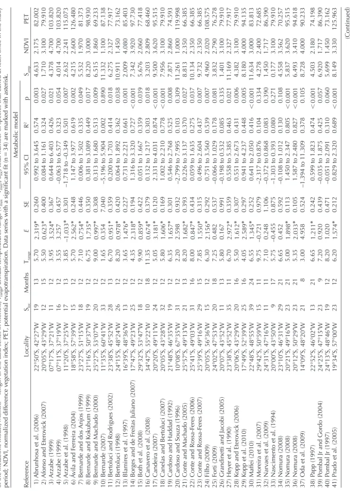
(4) 391. 22°50′S, 42°27′W 20°05′S, 43°29′W 07°17′S, 37°21′W 07°11′S, 37°19′W 11°20′S, 37°25′W 18°58′S, 57°39′W 23°27′S, 51°15′W 21°16′S, 50°37′W 25°27′S, 53°07′W 11°35′S, 60°41′W 23°38′S, 45°52′W 24°15′S, 48°24′W 16°39′S, 48°36′W 17°47′S, 49°23′W 29°32′S, 53°47′W 34°47′S, 55°22′W 20°20′S, 49°11′W 20°05′S, 43°28′W 21°48′S, 46°35′W 10°08′S, 67°35′W 25°57′S, 49°13′W 25°41′S, 49°03′W 25°39′S, 49°16′W 20°05′S, 56°36′W 24°02′S, 47°53′W 20°07′S, 43°52′W 23°38′S, 45°52′W 20°06′S, 43°29′W 17°49′S, 52°39′W 22°48′S, 48°55′W 29°42′S, 50°59′W 24°31′S, 47°16′W 20°00′S, 43°50′W 23°10′S, 46°31′W 20°21′S, 49°16′W 20°12′S, 50°29′W 14°09′S, 48°20′W 22°52′S, 46°02′W 24°25′S, 47°15′W 24°13′S, 48°46′W 19°34′S, 57°00′W. 38) Papp (1997) 39) Pombal Jr and Gordo (2004) 40) Pombal Jr (1997) 41) Prado et al. (2005). Locality. 1) Abrunhosa et al. (2006) 2) Afonso and Eterovick (2007) 3) Arzabe (1999) 4) Arzabe (1999) 5) Arzabe et al. (1998) 6) Ávila and Ferreira (2004) 7) Bernarde and dos Anjos (1999) 8) Bernarde and Kokubum (1999) 9) Bernarde and Machado (2000) 10) Bernarde (2007) 11) Bertoluci and Rodrigues (2002) 12) Bertoluci (1998) 13) Blamires et al. (1997) 14) Borges and de Freitas Juliano (2007) 15) Both et al. (2008) 16) Canavero et al. (2008) 17) Candeira (2007) 18) Canelas and Bertoluci (2007) 19) Cardoso and Haddad (1992) 20) Cardoso and Souza (1996) 21) Conte and Machado (2005) 22) Conte and Rossa-Feres (2006) 23) Conte and Rossa-Feres (2007) 24) Filho (2009) 25) Forti (2009) 26) Grandinetti and Jacobi (2005) 27) Heyer et al. (1990) 28) Kopp and Eterovick (2006) 29) Kopp et al. (2010) 30) Maffei (2010) 31) Moreira et al. (2007) 32) Narvaes et al. (2009) 33) Nascimento et al. (1994) 34) Nomura (2008) 35) Nomura (2008) 36) Nomura (2008) 37) Oda et al. (2009). Reference. 13 23 19 23. 19 12 11 16 17 15 18 19 20 33 28 26 13 25 18 10 24 32 19 31 21 31 29 15 20 11 35 20 25 39 15 11 9 29 23 23 21. Sloc. 21 9 12 12. 13 15 12 12 13 12 12 12 12 12 13 12 12 12 12 18 12 12 12 12 13 16 15 12 18 13 11 16 16 24 11 11 17 21 21 21 8. Months. 6.65 7.20 8.20 6.20. 5.70 5.50 3.95 3.55 3.85 5.70 7.10 6.75 9.00 1.65 6.70 8.20 3.65 4.35 9.90 11.35 5.05 5.80 6.35 2.20 8.20 8.00 7.85 6.30 7.25 5.80 6.70 5.50 4.05 6.55 9.75 7.10 5.75 6.65 5.00 5.35 3.00. Trange 0.992 to 3.645 0.084 to 1.161 0.644 to 6.403 –0.063 to 6.577 –1.718 to –0.349 1.147 to 3.977 0.006 to 1.502 0.381 to 3.089 0.313 to 1.680 –5.196 to 5.904 0.200 to 1.703 0.064 to 1.892 0.731 to 2.221 1.316 to 3.320 0.051 to 1.667 0.132 to 1.217 2.331 to 4.031 1.002 to 2.210 0.546 to 2.768 –2.799 to 7.995 0.226 to 3.137 0.059 to 1.635 0.496 to 2.604 0.751 to 3.560 –0.066 to 1.029 –0.198 to 0.532 0.558 to 5.385 0.551 to 2.673 0.941 to 4.237 0.641 to 2.050 –2.317 to 0.876 –0.372 to 0.868 –1.303 to 0.393 –0.108 to 1.012 1.450 to 2.347 1.587 to 2.480 –1.394 to 11.309 0.599 to 1.823 –0.035 to 1.875 –0.051 to 2.091 0.829 to 2.320. 0.260 0.400 0.367 0.457 0.301 0.248 0.446 0.350 0.308 7.040 0.359 0.420 0.227 0.194 0.422 0.379 0.120 0.169 0.301 0.932 0.393 0.434 0.315 0.292 0.537 0.991 0.359 0.307 0.297 0.252 0.979 1.106 0.875 0.592 0.113 0.105 0.524 0.242 0.439 0.471 0.212. 2.319* 0.623* 3.524* 3.257 –1.033* 2.562* 0.754* 1.735* 0.997* 0.354 0.951* 0.978* 1.476* 2.318* 0.859* 0.674* 3.181* 1.606* 1.657* 2.598 1.682* 0.847* 1.550* 2.156* 0.482 0.167 2.972* 1.612* 2.589* 1.345* –0.721 0.248 –0.455 0.452 1.898* 2.033* 4.958 1.211* 0.920 1.020 1.574*. 95% CI. SE. E. 0.474 0.425 0.310 0.689. 0.574 0.324 0.426 0.323 0.501 0.619 0.335 0.449 0.513 0.002 0.414 0.362 0.661 0.727 0.359 0.303 0.874 0.778 0.525 0.103 0.370 0.275 0.437 0.539 0.178 0.085 0.463 0.431 0.448 0.416 0.104 0.083 0.080 0.130 0.805 0.827 0.378. R2. Metabolic model.  0.001 0.057 0.060  0.001. 0.003 0.027 0.021 0.054 0.007 0.002 0.049 0.017 0.009 0.890 0.018 0.038 0.001  0.001 0.039 0.018  0.001  0.001 0.008 0.309 0.027 0.037 0.007 0.007 0.081 0.335 0.021 0.006 0.005  0.001 0.334 0.390 0.271 0.108  0.001  0.001 0.105. p. 4.503 6.920 5.699 8.149. 4.633 1.710 4.378 4.014 2.632 4.215 5.532 8.220 6.515 11.332 6.275 10.911 2.009 7.342 5.676 3.203 9.500 7.956 7.871 11.261 8.813 10.134 9.732 4.960 3.832 1.401 11.169 4.382 8.180 11.634 4.278 1.450 0.177 4.558 5.837 6.493 8.728. Samp. 74.198 86.390 73.162 125.963. 82.002 79.910 103.820 103.820 115.073 126.480 81.373 98.930 69.233 87.138 77.917 73.162 85.403 97.730 77.418 68.460 95.515 79.910 74.593 119.998 66.385 66.385 66.385 108.575 76.278 79.910 77.917 79.910 94.135 83.813 72.685 86.390 79.910 70.257 95.515 94.618 90.233. PET. (Continued). 2.180 1.717 1.450 3.330. 2.175 3.100 4.700 4.700 2.241 2.600 1.970 3.000 1.860 1.100 2.327 1.450 4.080 3.920 2.060 2.809 3.620 3.100 2.860 1.000 2.350 2.350 2.350 2.020 2.790 3.100 2.327 3.100 4.000 3.000 2.400 1.717 3.100 3.562 3.620 3.410 4.000. NDVI. Table 1. Local communities of Neotropical amphibians, statistical fits, estimated parameters, and their geographic location. The fit of the metabolic and the Samp parameter in the sinusoidal model is included. E, calling activation energy; 95% CI, 95% confidence interval of estimated slopes (E); R2  explained variance of the metabolic model, p  p-values of the metabolic model; Months  length of the data series in months; Trange, annual temperatures range (Tmax – Tmin); Sloc, total number of species that called at least once in the study period; NDVI, normalized difference vegetation index; PET, potential evapotranspiration. Data series with a significant fit (n  34) are marked with asterisk..

(5) 93.137 83.813 93.912 94.618 77.418 79.910 95.515 83.813 80.825 95.245 80.825 3.000 3.000 3.065 3.410 2.060 3.100 3.620 3.000 3.000 5.490 3.000 3.494 5.785 3.122 6.562 4.332 6.706 6.481 3.133 5.440 4.849 7.200 0.189 0.237 0.346  0.001 0.055 0.281  0.001 0.004 0.017 0.009  0.001 0.166 0.125 0.074 0.843 0.321 0.115 0.727 0.586 0.449 0.271 0.816 –0.349 to 1.557 –0.365 to 1.327 –0.712 to 0.270 2.056 to 3.856 –0.013 to 1.083 –0.647 to 1.999 1.385 to 3.488 0.446 to 1.742 0.401 to 3.250 0.872 to 5.496 1.444 to 2.899 0.709 0.799 1.018 0.137 0.460 0.878 0.194 0.266 0.350 0.350 0.150 0.604 0.481 –0.221 2.956* 0.535 0.676 2.437* 1.094* 1.825* 3.184* 2.172* 12 13 14 12 12 12 12 12 12 24 12 17 25 28 13 24 28 18 15 19 15 22. 5.25 6.45 3.30 6.10 10.25 6.35 5.05 6.50 6.40 3.55 6.40. PET NDVI Samp p R2. Metabolic model. 95% CI SE E Trange Months Sloc. the association between the standard error associated with E, with the range of temperatures used in the estimation. We fitted a metabolic model, lnSa  –E  1/kT  C (Allen et al. 2002), to anuran phenological data (Sa, species richness of calling males each month; k is Boltzmann’s constant (8.62  105eV K1, Gillooly et al. 2001); T, mean monthly temperature). We considered the fit of a non-linear model avoiding data transformation (O’Hara and Kotze 2010). However, as shown in the results section, these models had a poor performance on convergence and large error terms. Consequently, we worked with log-transformed data (Allen et al. 2002). In order to deal with observations of zerorichness on log-transformed data, a constant has to be added (Legendre and Legendre 2012). This constant may have the same order of magnitude as the significant digits of the variable to be transformed; for species richness this produces the classical transformation log(S  1) (Legendre and Legendre 2012). We further considered the performance of other values for the constant, such as 0.1 and 2. The alternative of excluding zero-values was not considered here because these are structural zeroes, that is, they are part of the biological phenomena under investigation, chiefly observed at low temperatures. Activation energies estimated from log-transformed data and non-linear fits were also compared with a Kolmogorov–Smirnov and a paired t-test. An additional matter of concern is that the estimations of parameter E from time series could be biased because of a lack of independence of residuals or non-linear association between log(S) and 1/KT (Pawar et al. 2016). Independence was evaluated with a Pearson’s autocorrelation for each time series and contrasting the estimated E values in models with or without a temporal variable that accounted for the autocorrelation. Non-linearity was evaluated considering a polynomic regression, estimating the Akaike weight of evidence for the polynomic model and the linear alternative (Burnham and Anderson 2004, Johnson and Omland  exp( −∆AIC / 2 )   w = 2004). i . Where R is the set of alterR  ∑ r =1 exp( −∆AIC /2 )   native models and ΔAIC the difference between each model and the best model. Akaike weights could be interpreted as the probability that a given model is the best model for the data (Burnham and Anderson 2004). Finally, in order to compare the distribution of E values calculated for each community (Table 1) with those calculated by a recent compilation of E values (activation energies estimated for the rise component of the temperature response curves of species interaction traits, see Table S3 in Dell et al. 2011), we performed a twosample Kolmogorov–Smirnov test and a paired t-test.. 392. 20°16′S, 40°28′W 22°59′S, 48°25′W 08°43′S, 35°50′W 20°11′S, 50°53′W 29°42′S, 53°42′W 20°31′S, 43°41′W 20°20′S, 49°11′W 22°59′S, 48°30′W 22°25′S, 47°33′W 07°25′S, 36°30′W 22°22′S, 47°28′W 42) Prado and Pombal (2005) 43) Rossa-Feres and Jim (1994) 44) Santos (2009) 45) Santos et al. (2007) 46) Santos et al. (2008) 47) Sao Pedro and Feio (2010) 48) Silva (2007) 49) Teixeira (2009) 50) Toledo et al. (2003) 51) Vieira et al. (2007) 52) Zina et al. (2007). Reference. Table 1. (Continued). Locality. i. r. Evaluating the variation in community activation energy. We performed a path analysis in order to evaluate a causal connection between environment, diversity, and the activation energy. We included the biological parameters estimated by the metabolic and sinusoidal models, and the set of environmental variables obtained for each locality. We.

(6) used structural equation modeling (SEM) to test the overall path diagram and the significance of each single connection between variables. The path analysis was used with maximum likelihood methods and standardized coefficient. To assess the significance of the overall path model, we used a c2 statistic computed by assessing the difference between the observed and expected covariance matrix derived from the proposed path model. A significant value (p  0.05) indicates that the data do not support the model. The explained variance for each endogenous variable is estimated as one minus the path coefficient between its associated error variable (Shipley 2000). Because our data matrix does not present multivariate normality based on kurtosis (using the mvnorm.kur.test function of the ICS package in R ver. 2.15.2, W  27.0852, w1  0.625, df1  20.000, w2  1.000, df2  1.000, p-value  0.01), we develop the Satorra–Bentler robust estimations of the Chi-squared statistic and standard errors. It corrects excessive kurtosis, problems in which the errors are not independent of their causal non-descendants, and is important for models with latent variables. We performed a SEM causally relating environmental conditions, activation energy, community seasonality, and local richness. Geographic trends in environmental variables are mutually correlated and are properly captured in a latent variable, which is similar to the axis of a principal component analysis (Shipley 2000). Consequently, we considered a latent variable ‘Environment’ connected with NDVI, PET, and latitude. This ‘Environment’ variable was connected with activation energy and the amplitude of the temporal variation on community richness; which was also determined by local species richness. Finally, an effect of activation energy on the amplitude of variation in species richness was considered. We also evaluated alternative path models, including the putative role of the environment upon local species richness (Sloc); but this path connection was rejected as a plausible causal explanation of data (Supplementary material Appendix 2). All SEM models were fitted using the R-package lavaan (Rosseel 2012). To incorporate community phylogenetic distances in our analysis, we reconstructed the phylogeny of 361 species of Neotropical anurans (for methodological details and phylogenetic tree see Supplementary material Appendix 3). Then we estimated the mean pairwise phylogenetic distance (MPD). This index finds for each taxon in a community the average phylogenetic distance to all taxa in another community, and calculates the mean using the COMDIST module of PHYLOCOM software (Webb et al. 2008). Next, we compared the environmental (Euclidean distances of community environment measured as: NDVI, PET, and latitude ordered by the two first axes of a principal component analysis) and MPD distance matrices with the matrix of community activation energy distances (each distance was calculated as the activation energy of community A minus the activation energy of community B) using a simple Mantel test (10 000 permutations). Finally, we explored the link between the community activation energy, and phylogeny or environment, using partial Mantel test. (10 000 permutations). In order to describe the activation energy matrix, we calculated the partial correlation with phylogeny after removing the effect of environment, and then calculated the partial correlation with environment after removing the contribution of phylogeny (Naisbit et al. 2012).. Results The number of species engaged in calling activities was better explained by the random intercept and slope model, which had the lowest AIC value (AIC  1407.65) in comparison with the random intercept model (AIC  1440.66) and the random effects model (AIC  1621.17). The former model presents high values of standard deviation of the intercept (28.62) and of the slope (0.74eV) showing the relevance of community idiosyncrasy (Fig. 2). This variation in slope highlights the importance of analyzing the activation energy as a biological variable. Out of the 52 phenological community data-series analyzed, 35 fit significantly the metabolic model, with a percentage of the explained variance ranging from 27.5 to 87.4%. We considered the case 5 (Arzabe et al. 1998) as an outlier because it presents an extreme value of E (–1.033eV). Indeed, Arzabe et al. (1998) suggested that the hydroperiod was the mayor factor influencing and maintaining assemblages of anurans in that location. So the main mechanisms operating would be the regulation of hydric demands and not temperature related. The mean and median of E values estimated is 1.80eV (standard error  0.14eV) and 1.67eV, respectively (n  34). The distribution of the activation energy shows significant differences with the right skewness distribution presented by Dell et al. (2011) for the responses of positive and negative traits associated with species interactions (two-sample Kolmogorov–Smirnov test: D  0.648, p-value  0.001). Further, the present distribution of activation energies did not differ from a normal distribution (Shapiro–Wilk test of normality: W  0.957, p-value  0.204) (Fig. 3). The 95% confidence interval of the mean activation energy of the calling activity (1.53 to 2.08eV) excludes the empirical value of approximately 0.65eV (Huey and Kingsolver 2011) and also the range of values 0.2 to 1.2eV proposed by Gillooly et al. (2001) for a wide range of thermal dependence of amphibians. The strong support for the linear model relating log(S) and 1/KT (W.linear  0.98; Supplementary material Appendix 4) does not support an overestimation of E because of non-linear trends. The analysis of residuals reported a significant autocorrelation in 17 of the 52 cases. So we included a temporal component to the equation (lnSa  –E  1/kT  month  C) and estimated the slope (i.e. the activation energy E). In this case eighteen models had a significant fit (p-value  0.05) and twenty-eight a marginal fit (p-value  0.1). We did not find differences between mean values of E estimated from both models using either all fitted values (Welch two sample t-test, N1  N2  52, t  0.966, df  101.06, p-value  0.337),. 393.

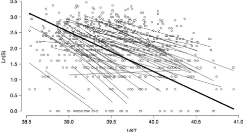
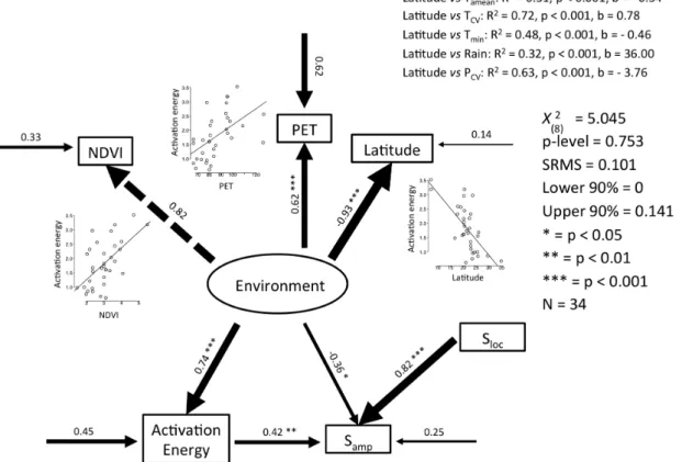
(7) Figure 2. Fitted random intercept and slope model with the reciprocal temperature in Kelvin multiplied by Boltzmann’s constant (k) as independent variable, and as dependent variables the natural logarithm of the number of species with calling behavior per month. The black line represents the fitted values for all communities, and the grey lines represent the fit for local communities. Dots represent the number of species that call in a particular month of a particular community.. or only the significant fits (Welch two sample t-test, N1  34, N2  28, t  0.560, df  51.484, p-value  0.578, mean1  1.804, mean2  1.675). Similarly, when comparing the distributions of E values, we did not find significant differences either (two-sample Kolmogorov–Smirnov test, D  0.132, p-value  0.910). Based on this result, where E does not differ significantly on their mean and distribution no matter if it is estimated considering residual autocorrelation or not, we opted for the initial estimates. Finally, the standard errors associated with estimated E values were not associated with the range of temperatures involved in the estimation (F1,49  0.031; p-value  0.86). An outlier with no significant E and very large standard error was excluded in this estimation. Further, when only significant E values were considered, a positive association between estimated. Figure 3. Activation energy histogram. E, activation energy calculated with the metabolic model presented by Allen et al. (2002): lnSa  –E  (1/kT)  C; S, number of species with calling behavior per month; T, mean month temperature in Kelvin degrees; k  Boltzmann constant  8.62  10–5 eV K–1; calculated with the 34 of 52 data series with a significant fit.. 394. E and the range of temperatures was observed (F1,32  9.05; p-value  0.005; R2  0.20). This contradict the expected negative association because an artifact from a unimodal rate-temperature relationship (Pawar et al. 2016). The non-linear models for Sa frequently failed to converge, requiring very large number of iterations and evaluation of several alternative starting values to achieve convergence. Further, no difference was detected in the distribution (two-sample Kolmogorov–Smirnov test: D  0.098, p-value  0.97) and mean value (paired t49  1.01, p-value  0.32) of E estimated with non-linear fit or logtransformed richness (log(Sa  1)), but standard errors from non-linear models were significantly larger (paired t49  4.36, p-value  0.0001) than those estimated by the linear model. However, the use of other constants (c  0.1 and c  2) determined significant deviation between E estimated with non-linear fit (paired t49  –2.88, p-value  0.006; paired t49  2.56, p-value  0.013) or log-transformed richness (paired t49  –4.29, p-value  0.0001; paired t49  6.30, p-value  0.0001). Consequently, we carried out all analyses using the log-transformed linear model adding a constant c  1, because it displays a better performance and because it is amenable of analysis with mixed models (Zuur et al. 2009). The path analysis and simple and partial Mantel tests were performed with the 34 communities for which we found a significant fit to the linearized metabolic model. The path analysis model shown in Fig. 4 explained 55% of the variance in calling activation energy (E), showing the main role of the environment (represented by a latent variable constructed by NDVI, PET, and latitude) as the main driver of E. The latent variable shows a positive correlation with productivity variables (NDVI and PET) and calling activation energy; and negative correlation with latitude and calling seasonality (Samp). This means that with an increase in latitude we find a decrease in system productivity, greater calling seasonality,.

(8) Figure 4. Evaluation of the putative role of the environment and community richness on the activation energy of anuran calling activity. Sloc, total number of species that call at least once in the study period; NDVI, normalized difference vegetation index; PET, potential evapotranspiration; Samp is a parameter of the sinusoidal function: S  Smean  Samp sin [2  p  (month  c)/12]; S, number of species that call in a particular month; Samp, amplitude of the sinusoidal function; Smean, mean value of S estimated from the sinusoidal function. Paths values are standardized effects. Values of 1 mean completely causal link and a value of 0 mean no causal link. Arrow width represents the strength of the causal link. In the figure was included the result of correlations of latitude as independent variable with mean annual temperature  Tamean, coefficient of variation in annual temperature  TCV, minimum temperature  Tmin, total annual rainfall  rain and coefficient of variation in annual precipitation  PCV; external arrows represent variances unexplained by the model, and the explained variance for endogenous variables is represented by one minus the path coefficient between its associated error variable. SRMS, standardized root mean square error.. and smaller calling activation energy. We also found a positive connection between calling activation energy and calling seasonality. Latitude also showed significant correlation with annual mean temperature Tamean (R2  0.31, p-value  0.001, b  –0.34), coefficient of variation in mean monthly temperature TCV (R2  0.72, p-value  0.001, b  0.78), minimum temperature of coldest month Tmin (R2  0.48, p-value  0.001, b  –0.46), rain (R2  0.32, p-value  0.001, b  36.00), and coefficient of variation in annual precipitation PCV (R2  0.63, p-value  0.001, b  –3.76). The simple Mantel test reported a significant association between the environmental and MPD matrices (rpearson  0.47, p-value  0.0001) (Fig. 5 top). Similarly, the partial Mantel tests between the activation energy matrix with the environment similarity matrix after removing the effect of phylogeny was significant (rpearson  0.35, p-value  0.0001), but the correlation between the activation energy and phylogeny, after removing the effect of environment, was. Figure 5. (A) Results of partial and simple Mantel test between the environmental (NDVI, PET, and latitude), phylogenetic (MPD distance), and activation energy distance matrices. (B) Results of the simple Mantel test between the phylogenetic (MPD distance) and activation energy distance matrices. Arrow width represents the strength of the link. **p  0.01; ***p  0.001.. 395.

(9) not significant (rpearson  0.08, p-value  0.154) (Fig. 5 top). When we explored a simple Mantel test between phylogeny and activation energy matrix we found a significant association (rpearson  0.26, p-value  0.002) (Fig. 5 bottom).. Discussion Understanding the observed variation in activation energy (E) among organisms and environments represents a novel challenge for the MTE (Stegen et al. 2009, Dell et al. 2011, 2014). In this contribution we show that variance in E is associated with ecological and evolutionary processes. It has been common to analyze the variability in E by combining data from different locations that differ in area, community attributes and phylogenetic similarity, which can potentially introduce biases in the estimation of activation energies and their determinants (Price et al. 2012, Storch 2012, Segura et al. 2015). Our analyses control for these potential biases by working with assemblages of locally coexisting species and explaining changes in E by considering the environments they experience and the attributes they possess. In this sense, our study provides a more ecological view of the factor affecting variability in E and at the same time overcomes previous criticisms to MTE. In particular it does this because it involves: 1) changes in community richness (i.e. number of species in activity per month) with temperature but without changes in area (Šímová et al. 2011); 2) a reasonable constancy in total community abundance since changes mostly reflect the proportion of active individuals (Storch 2012); 3) a single species pool, and thus no change in the phylogenetic structure of communities at different temperatures (generally geographical, Kaspari et al. 2004, Algar et al. 2007, Hawkins et al. 2007); and 4) changes in richness with temperature are decoupled from mutation and speciation rates, which is an alternative metabolic connection between temperature and richness (Gillooly et al. 2005, Allen et al. 2006, 2007). An important difference between previous analyses of variation in species richness in the MTE framework, and the present analysis focused on the number of calling species, should be highlighted (Allen et al. 2002). The MTE considered the individuals’ energetic demand – standard metabolic rate – and its dependence on temperature to predict trends in species richness (Allen et al. 2002, Segura et al. 2015). Here, the metabolic rate affected by temperature also involves the energetic expenditure of calling (Gillooly and Ophir 2010, Ophir et al. 2010, Ziegler et al. 2016). Everything else being equal, predictions of MTE for the association between species richness and temperature are expected to meet when the focus is the number of species calling. Accounting for the idiosyncrasy of each system, we believe that the seasonal variation in the richness and abundance of ectotherms represents an ideal model system to study the connection between organismal energetics and community structure. Phenological patterns could be addressed as a temporal version of the ‘more-individuals’ hypothesis (Gaston 2000), where an increase in energy availability in some months of. 396. a year would lead to higher abundances of individuals (via increased reproduction and migration) and consequently more species (Gaston 2000, Storch 2012). An alternative but not exclusive hypothesis considers that ectothermic species have different activation thresholds or differential tolerances to the harsh period (e.g. lower temperatures) and alternate between reduction on vital activities in unfavorable conditions and activation during favorable ones (McNab 2002, Angilletta 2009). In this context, intraspecific variability in calling behavior, reflected in temporal changes in abundance within species, could be a main component of amphibians’ phenology, not captured when considering species richness, which could have important implications on the estimation of E. This effect of temperature upon ectotherm abundance is important and requires further study. Our results showed values of E (mean  1.80eV) significantly higher than what was expected by the MTE (i.e. 0.65eV or the interval 0.2–1.2eV, West et al. 1997, 1999, Gillooly et al. 2001, Downs et al. 2008), meaning that amphibians’ calling behavior is highly sensitive to temperature variation. This difference in activation energies could be reflecting the nature of the activity involved – reproduction (Dell et al. 2011, 2014), or a statistical artifact related to the range of temperatures from which activations energies were estimated (Pawar et al. 2016). We consider that our analyses discard the artifact interpretation. The source of an overestimation of E is the potential nonlinear association between log(S) and 1/KT (Pawar et al. 2016). This non-linearity was not observed in our dataset, where the probability of the linear model is close to 1.0 in comparison to its alternatives. Discarding non-linearity, the relatively narrow range of temperatures experienced by amphians’ communities could determine an over dispersion of estimated E – large standard errors (Pawar et al. 2016). It should be highlighted that the present dataset follows the opposite trend, with an increase in standard errors within the temperature range (Supplementary material Appendix 4 Fig. A6). This suggests that a biological process is reverting the statistical expectation. In this sense, the range of temperature is closely related with latitude (r-square  0.82; p  0.001) and consequently the trend in activation energy and its standard error are probably related with trends in physiological mechanisms along the latitudinal gradient. Alternative source of biases such as autocorrelation in richness and the log(S  1) transformation of data were not identified as significant determinants of reported E-values. Accordingly, it should be highlighted that while nonlinear fits could properly account for a trend on average values, it could fail to properly deal with an error structure that increases exponentially with the independent variable. Finally, our global estimation of thermal dependence (activation energy) is obtained with a mixed model that combines information from 52 datasets. Consequently, the putative effects of temperature range on accuracy and precision discard by the increase in accuracy because the mixed model is using a large amount of information and accounts for a large part of estimated errors when the general thermal dependence is assessed (Zuur et al. 2009). Our broad consideration.

(10) of alternative sources of bias on estimated E-values and the use of mixed model with a large database suggest that the reported high activation energy for amphibians’ community phenology is indeed a biological phenomenon and not a methodological artifact. On the other hand, and further supporting a biological interpretation of the high E-values herein reported, reproduction is the largest component of the entire annual energy budget of anurans while calling behavior is tightly coupled to individual fitness (Wells 2007, Ophir et al. 2010). The morphological and biochemical basis of this ability is centered in the muscles of call production: trunk and laryngeal muscles, which differ from leg muscles in allowing anurans to have an intense aerobic metabolism (more aerobic fiber types, higher concentrations of mitochondria, capillaries, and enzymes) (Wells 2007). In this context, it is not surprising that our estimations of activation energy exceed by twice the activation energies values reported for other behaviors (Gillooly et al. 2001, Dell et al. 2011). Environment–diversity relationship is the result of the interplay between environmental conditions, organisms’ attributes, and the effect of evolutionary history on these attributes (Marquet et al. 2004b, Shipley 2010). Calling is an energetically expensive activity that pushes anurans to their limits and brings an opportunity to explore their physiological constraints (Wells 2007). We found that at higher latitudes, where phenologies are more seasonal and environments have lower primary productivity, communities tend to show low E values. Apparently, organisms are coupling what the environment offers with their own metabolic demands for calling. The observed trend of reduction in E with latitude raises questions: how do anurans call in less energetic environments? Or how do anurans reduce the energetic demands of calling? In this vein, a correlation has been observed between the metabolic demand to call and the size of the muscular system of calling (Wells 2007, Ophir et al. 2010). So, we hypothesize that as latitude increases, there is a reduction in calling parameters (e.g. sound frequency, call rate, call duration, sound power; Gillooly and Ophir 2010, Ophir et al. 2010) associated with the downsizing of the muscular system of calling (e.g. anuran trunk muscles; Wells 2007, Ophir et al. 2010). Our results also show that an increase in the activation energy results in phenologies with stronger seasonality, when other abiotic variables (i.e. NDVI, PET, latitude) are fixed. If the activation energy is low, organisms can be relatively insensitive to environmental seasonality, showing low seasonality in calling phenologies. The detected connections among communities’ phylogenetic structure, environmental conditions, and activation energy is interesting in that they relate biodiversity structure and their determinants with MTE. The environmental–phylogeny association detected in the Mantel tests evidences both niche conservatisms and community filtering on conserved traits, as a determinant of amphibian communities (see also Wiens et al. 2006, Buckley and Jetz 2007, Gouveia et al. 2013). Further, the environment–activation energy association supports the view of activation energy as. a parameter that encapsulates main components of the relationship between energy use, environmental conditions, and organisms physiology, being a meaningful parameter at different biological levels (Brown et al. 2004, Dell et al. 2011). The environment–activation energy relationship suggests that species or individuals within species are actively filtered depending on their activation energies and the local environments (Violle et al. 2012), which implies that there are limits to the flexibility in activation energy (Ziegler et al. 2011). The ecological concept of activation energy is being reconsidered from a fixed attribute of higher taxa (e.g. amphibians) to a parameter that depends of the species involved and the traits considered (Dell et al. 2011, 2014). Thermal dependence is a flexible trait (McNab 2002), and the role of this flexibility on observed activation energies should be an important determinant of observed patterns. Moving from the existence of a universal thermal dependence controlling biological processes (Brown et al. 2004, Huey and Kingsolver 2011) to address the activation energy as a variable biological trait, represents a challenge but also an opportunity for research (Stegen et al. 2009, Humphries and McCann 2014), because this variation may reflect the ecological and evolutionary nature of the trait (Dell et al. 2011, 2014, Huey and Kingsolver 2011). The MTE has been combined with other theories in order to reach new insights and the understanding of the biological complexity at different levels and scales (e.g. life-history theory, the neutral theory of biodiversity, food web theory; Price et al. 2012). In this vein, we found that incorporating the MTE to the phenological framework makes a contribution to improving our understanding of how metabolism relates to patterns and processes in local communities (Tilman et al. 2004). Acknowledgements – We thank Arley Camargo for his contributions to the construction of the phylogenetic tree of the Neotropical anurans used in this work and to Jamie Gillooly for helpful comments that have significantly improved the manuscript. We thank Ivan Barria for editing Fig. 1. Funding – AC received a fellowship from the Vicerrectoría Adjunta de Investigación y Doctorado-PUC, Chile, and the support of grants CONICYT PFB-23, ICM P05-002 and FB-0002-2014. MA thanks FCE_2014_104763.. References Abrunhosa, P. A. et al. 2006. Anuran temporal occupancy in a temporary pond from the atlantic rain forest, south-eastern brazil. – Herpetol. J. 16: 115–122. Afonso, L. G. and Eterovick, P. C. 2007. Spatial and temporal distribution of breeding anurans in streams in southeastern Brazil. – J. Nat. Hist. 41: 949–963. Algar, A. C. et al. 2007. A test of metabolic theory as the mechanism underlying broad-scale species-richness gradients. – Global Ecol. Biogeogr. 16: 170–178. Allen, A. P. and Gillooly, J. F. 2006. Assessing latitudinal gradients in speciation rates and biodiversity at the global scale. – Ecol. Lett. 9: 947–954.. 397.

(11) Allen, A. P. et al. 2002. Global biodiversity, biochemical kinetics, and the energetic-equivalence rule. – Science 297: 1545–1548. Allen, A. P. et al. 2006. Kinetic effects of temperature on rates of genetic divergence and speciation. – Proc. Natl Acad. Sci. USA 103: 9130–9135. Allen, A. P. et al. 2007. Recasting the species–energy hypothesis: the different roles of kinetic and potential energy in regulating biodiversity. – In: Storch, D. et al. (eds), Scaling biodiversity. Cambridge Univ. Press, pp. 283–299. Angilletta, J. M. J. 2009. Thermal adaptation: a theoretical and empirical synthesis. – Oxford Univ. Press. Arzabe, C. 1999. Reproductive activity patterns of anurans in two different altitudinal sites within the Brazilian Caatinga. – Rev. Bras. Zool. 16: 851–864. Arzabe, C. et al. 1998. Anuran assemblages in Crasto Forest ponds (Sergipe State, Brazil): comparative structure and calling activity patterns. – Herpetol. J. 8: 111–113. Ávila, R. W. and Ferreira, V. L. 2004. Riqueza e densidade de vocalizações de anuros (Amphibia) em uma área urbana de Corumbá, Mato Grosso do Sul, Brasil. – Rev. Bras. Zool. 21: 887–892. Bernarde, P. S. 2007. Ambientes e temporada de vocalização da anurofauna no Município de Espigão do Oeste, Rondônia, Sudoeste da Amazônia – Brasil (Amphibia: Anura). – Biota Neotrop. 7: 87–92. Bernarde, P. S. and dos Anjos, L. 1999. Distribução espacial e temporal da anurofauna no Parque Estadual Mata dos Godoy, Londrina, Paraná, Brasil (Amphibia: Anura). – Comun. Mus. Cienc. Tecnol. PUCRS Ser. Zool. 12: 127–140. Bernarde, P. S. and Kokubum, M. N. C. 1999. Anurofauna do Municipio de Guararapes, Estado de São Paulo, Brasil (Amphibia: Anura). – Acta Biol. Leopold. 21: 89–97. Bernarde, P. S. and Machado, R. A. 2000. Riqueza de espécies, ambientes de reprodução e temporada de vocalização da anurofauna em Três Barras do Paraná, Brasil (Amphibia: Anura). – Cuad. Herpetol. 14: 93–104. Bertoluci, J. 1998. Annual patterns of breeding activity in Atlantic rainforest anurans. – J. Herpetol. 32: 607–611. Bertoluci, J. and Rodrigues, M. T. 2002. Seasonal patterns of breeding activity of Atlantic Rainforest anurans at Boracéia, southeastern Brazil. – Amphibia-Reptilia 23: 161–167. Blair, W. 1961. Calling and spawning seasons in a mixed population of anurans. – Ecology 42: 99–110. Blamires, D. et al. 1997. Padroes de distribucao e analise de canto em uma comunidade de anuros no Brasil central. Contribucao ao conhecimento ecológico do cerrado. – Trabalhos selecionados do 3° congresso de ecología do Brasil, Univ. de Brasilia, pp. 185–190. Boquimpani-Freitas, L. et al. 2007. Temporal niche of acoustic activity in anurans: interspecific and seasonal variation in a neotropical assemblage from south-eastern Brazil. – AmphibiaReptilia 28: 269–276. Borges, F. J. A. and de Freitas Juliano, R. 2007. Distribuição espacial e temporal de uma comunidade de anuros do município de Morrinhos, Goiás, Brasil (Amphibia: Anura). – Neotrop. Biol. Conserv. 2: 21–27. Both, C. et al. 2008. An austral anuran assemblage in the Neotropics: seasonal occurrence correlated with photoperiod. – J. Nat. Hist. 42: 205–222. Bradshaw, W. E. and Holzapfel, C. M. 2007. Evolution of animal photoperiodism. – Annu. Rev. Ecol. Evol. Syst. 38: 1–25.. 398. Brown, J. H. 2014. Why are there so many species in the tropics? – J. Biogeogr. 41: 8–22. Brown, J. H. and Maurer, B. A. 1986. Body size, ecological dominance and Cope’s rule. – Nature 324: 248–250. Brown, J. H. et al. 2004. Toward a metabolic theory of ecology. – Ecology 85: 1771–1789. Buckley, L. B. and Jetz, W. 2007. Environmental and historical constraints on global patterns of amphibian richness. – Proc. R. Soc. B 274: 1167–1173. Burnham, K. P. and Anderson, D. R. 2004. Multimodel inference: understanding AIC and BIC in model selection. – Soc. Methods Res. 33: 261–304. Canavero, A. et al. 2008. Calling activity patterns in an anuran assemblage: the role of seasonal trends and weather determinants. – North-West. J. Zool. 4: 29–41. Canavero, A. et al. 2009. Geographic variations of seasonality and coexistence in communities: the role of diversity and climate. – Austral Ecol. 34: 741–750. Candeira, C. P. 2007. Estrutura de comunidades e influência da heterogeneidade ambiental na diversidade de anuros em área de pastagem no sudeste do Brasil. – Inst. de Biociências Letras e Ciências Exatas, Univ. Estadual Paulista. Canelas, M. A. S. and Bertoluci, J. 2007. Anurans of the Serra do Caraça, southeastern Brazil: species composition and phenological patterns of calling activity. – Iheringia Sér. Zool. 97: 21–26. Cardoso, A. J. and Haddad, C. F. B. 1992. Diversidade e turno de vocalizações de anuros em comunidade neotropical. – Acta Zool. Lilloana 41: 93–105. Cardoso, A. J. and Souza, M. B. 1996. Distribucao temporal e espacial de anfibios anuros no Seringal Catuaba, Estado do Acre, Brasil. – In: Pefaur, J. E. (ed.), Herpetología Neotropical. Acta II Congreso Latinoamericano de Herpetología. Univ. de los Andes, pp. 271–291. Caruso, T. et al. 2010. Testing metabolic scaling theory using intraspecific allometries in Antarctic microarthropods. – Oikos 119: 935–945. Conte, C. E. and Machado, R. A. 2005. Riqueza de espécies e distribução espacial e temporal em comunidade de anuros (Amphibia, Anura) em uma oocalidade de Tijucas do Sul, Paraná, Brasil. – Rev. Bras. Zool. 22: 940–948. Conte, C. E. and Rossa-Feres, D. C. 2006. Diversidade e ocorrência temporal da anurofoauna (Amphibia, Anura) em São José dos Pinhais, Paraná, Brasil. – Rev. Bras. Zool. 23: 162–175. Conte, C. E. and Rossa-Feres, D. C. 2007. Riqueza e distribuição espaço-temporal de anuros em um remanescente de Floresta de Araucária no sudeste do Paraná. – Rev. Bras. Zool. 24: 1025–1037. Crump, M. L. 1974. Reproductive strategies in a tropical anuran community. – Miscellaneous Publ. Mus. Nat. Hist. Univ. of Kansas 61: 1–68. Dell, A. I. et al. 2011. Systematic variation in the temperature dependence of physiological and ecological traits. – Proc. Natl Acad. Sci. USA 108: 10591–10596. Dell, A. I. et al. 2014. Temperature dependence of trophic interactions are driven by asymmetry of species responses and foraging strategy. – J. Anim. Ecol. 83: 70–84. Downs, C. J. et al. 2008. Scaling metabolic rate with body mass and inverse body temperature: a test of the Arrhenius fractal supply model. – Funct. Ecol. 22: 239–244. Ehnes, R. B. et al. 2011. Phylogenetic grouping, curvature and metabolic scaling in terrestrial invertebrates. – Ecol. Lett. 14: 993–1000..

(12) Emerson, K. J. et al. 2008. Concordance of the circadian clock with the environment is necessary to maximize fitness in natural populations. – Evolution 62: 979–983. Enquist, B. J. et al. 2009. Extensions and evaluations of a general quantitative theory of forest structure and dynamics. – Proc. Natl Acad. Sci. USA 106: 7046–7051. Filho, P. L. 2009. Padões reprodutivos de anfíbios anuros em um agroecossistema no estado de Mato Grosso do Sul. – Univ. Federal de Mato Grosso do Sul. Forrest, J. and Miller-Rushing, A. J. 2010. Toward a synthetic understanding of the role of phenology in ecology and evolution. – Phil. Trans. R. Soc. B 365: 3101–3112. Forti, L. R. 2009. Temporada reprodutiva, micro-habitat e turno de vocalização de anfíbios anuros em lagoa de Floresta Atlântica, no sudeste do Brasil. – Rev. Bras. Zoociênc. 11: 89–98. Gaston, K. J. 2000. Global patterns in biodiversity. – Nature 405: 220–227. Gillooly, J. F. and Ophir, A. G. 2010. The energetic basis of acoustic communication. – Proc. R. Soc. B 277: 1325–1331. Gillooly, J. F. et al. 2001. Effects of size and temperature on metabolic rate. – Science 293: 2248–2251. Gillooly, J. F. et al. 2005. The rate of DNA evolution: effects of body size and temperature on the molecular clock. – Proc. Natl Acad. Sci. USA 102: 140–145. Gillooly, J. F. et al. 2007. Effects of metabolic rate on protein evolution. – Biol. Lett. 3: 655–659. Gouveia, S. F. et al. 2013. Nonstationary effects of productivity, seasonality, and historical climate changes on global amphibian diversity. – Ecography 36: 104–113. Grandinetti, L. and Jacobi, C. M. 2005. Distribuição estacional e espacial de uma taxocenose de anuros (Amphibia) em uma área antropizada em Rio Acima – MG. – Lundiana 6: 21–28. Hawkins, B. A. et al. 2007. A global evaluation of metabolic theory as an explanation for terrestrial species richness gradients. – Ecology 88: 1877–1888. Heyer, R. et al. 1990. Frogs of Boracéia. – Arquivos de Zool. 31: 231–410. Heyer, W. R. et al. 1994. Measuring and monitoring biological diversity, standard methods for amphibians. – Smithsonian Inst. Hijmans, R. J. et al. 2005. Very high resolution interpolated climate surfaces for global land areas. – Int. J. Climatol. 25: 1965–1978. Hilborn, R. and Mangel, M. 1997. The ecological detective confronting models with data. – Princeton Univ. Press. Huey, R. B. and Kingsolver, J. G. 2011. Variation in universal temperature dependence of biological rates. – Proc. Natl Acad. Sci. USA 108: 10377–10378. Humphries, M. M. and McCann, K. S. 2014. Metabolic ecology. – J. Anim. Ecol. 83: 7–19. Inger, R. F. 1969. Organization of communities of frogs along small rain forest stream in Sarawak. – J. Anim. Ecol. 38: 123–148. Jenouvrier, S. and Visser, M. E. 2011. Climate change, phenological shifts, eco-evolutionary responses and population viability: toward a unifying predictive approach. – Int. J. Biometeorol. 55: 905–919. Johnson, J. B. and Omland, K. S. 2004. Model selection in ecology and evolution. – Trends Ecol. Evol. 19: 101–108. Kaspari, M. et al. 2004. Energy gradients and the geographic distribution of local ant diversity. – Oecologia 140: 407–413. Kopp, K. and Eterovick, P. C. 2006. Factors influencing spatial and temporal structure of frog assemblages at ponds in southeastern Brazil. – J. Nat. Hist. 40: 1813–1830.. Kopp, K. et al. 2010. Distribuição temporal e diversidade de modos reprodutivos de anfíbios anuros no Parque Nacional das Emas e entorno, estado de Goiás, Brasil. – Iheringia Sér. Zool. 100: 192–200. Kronfeld-Schor, N. and Dayan, T. 2003. Partitioning of time as an ecological resource. – Annu. Rev. Ecol. Evol. Syst. 34: 153–181. Legendre, P. and Legendre, L. 2012. Numerical ecology, 3rd ed. – Elsevier Science. Maffei, F. 2010. Diversidade e uso do habitat de comunidades de anfíbios anuros em Lençóis Paulista, Estado de São Paulo. – Inst. de Biociências de Botucatu, Univ. Estadual Paulista. Marquet, P. A. and Taper, M. L. 1998. On size and area: patterns of mammalian body size extremes across landmasses. – Evol. Ecol. 12: 127–139. Marquet, P. A. et al. 1990. Scaling population density to body size in rocky intertidal communities. – Science 250: 1125–1127. Marquet, P. A. et al. 2004a. Metabolic ecology: linking individuals to ecosystems. – Ecology 85: 1794–1796. Marquet, P. A. et al. 2004b. Diversity emerging: towards a deconstruction of biodiversity patterns. – In: Lomolino, M. and Heaney, L. (eds), Frontiers of biogeography: new directions in the geography of nature. Sinauer Associates, pp. 191–209. McNab, B. K. 2002. The physiological ecology of vertebrates: a view from energetics. – Comstock/Cornell Univ. Press. Moreira, L. F. B. et al. 2007. Calling period and reproductive modes in an anuran community of a temporary pond in southern Brazil. – S. Am. J. Herpetol. 2: 129–135. Morin, P. J. 1999. Community ecology. – Blackwell Science. Munch, S. B. and Salinas, S. 2009. Latitudinal variation in lifespan within species is explained by the metabolic theory of ecology. – Proc. Natl Acad. Sci. USA 106: 13860–13864. Naisbit, R. E. et al. 2012. Phylogeny versus body size as determinants of food web structure. – Proc. R. Soc. B 279: 3291–3297. Narvaes, P. et al. 2009. Composição, uso de hábitat e estações reprodutivas das espécies de anuros da floresta de restinga da Estação Ecológica Juréia-Itatins, sudeste do Brasil. – Biota Neotrop. 9: 1–7. Nascimento, L. B. et al. 1994. Distribuição estacional e ocupação ambiental dos anfíbios anuros da área de proteção da captação da Mutuca (Nova Lima, MG). – BioScience 2: 5–12. Nomura, F. 2008. Padrões de diversidade e estrutura de taxocenoses de anfíbios anuros: análise em multiescala espacial. Instituto de Biociências. – Univ. Estadual Paulista ‘Júlio de Mesquita Filho’. Oda, F. H. et al. 2009. Taxocenose de anfíbios anuros no Cerrado do Alto Tocantins, Niquelândia, Estado de Goiás: diversidade, distribuição local e sazonalidade. – Biota Neotrop. 9: 219–232. O’Hara, R. B. and Kotze, D. J. 2010. Do not log-transform count data. – Methods Ecol. Evol. 1: 118–122. Ophir, A. G. et al. 2010. Energetic cost of calling: general constraints and species-specific differences. – J. Evol. Biol. 23: 1564–1569. Papp, M. G. 1997. Reproducção de anuros (Amphibia) em duas lagoas de altitude na Serra da Mantiqueira. – Univ. Estadual de Campinas, UNICAMP. Pau, S. et al. 2011. Predicting phenology by integrating ecology, evolution and climate science. – Global Change Biol. 17: 3633–3643. Pawar, S. et al. 2016. Real versus artificial variation in the thermal sensitivity of biological traits. – Am. Nat. 187: E41–E52. Pinheiro, J. et al. 2013. nlme: linear and nonlinear mixed effects models. – R package ver. 3.1-108.. 399.

(13) Pombal Jr, J. P. 1997. Distribução espacial e temporal de anuros (Amphibia) em uma poça permanente na Serra de Paranapiacaba, sudeste do Brasil. – Rev. Bras. Biol. 57: 583–594. Pombal Jr, J. P. and Gordo, M. 2004. Anfíbios anuros da Juréia. – In: Marques, O. V. and Wânia, D. (eds), Estação Ecológica Juréia-Itatins. Ambioente Físico, Flora e Fauna. Holos, pp. 243–256. Prado, C. P. A. et al. 2005. Breeding activity patterns, reproductive modes, and habitat use by anurans (Amphibia) in a seasonal environment in the Pantanal, Brazil. – Amphibia-Reptilia 26: 211–221. Prado, G. M. and Pombal, J. J. P. 2005. Distribução espacial e temporla dos anuros em um brejo da reserva biológica de Duas Bocas, sudeste do Brasil. – Arq. Mus. Nac. 63: 685–705. Price, C. A. et al. 2012. Testing the metabolic theory of ecology. – Ecol. Lett. 15: 1465–1474. Rangel, T. F. L. V. B. et al. 2006. Towards an integrated computational tool for spatial analysis in macroecology and biogeography. – Global Ecol. Biogeogr. 15: 321–327. Richards, S. A. 2005. Testing ecological theory using the informationtheoretic approach: examples and cautionary results. – Ecology 86: 2805–2814. Rossa-Feres, D. and Jim, J. 1994. Distrrbuição sazonal em comunidades de anfíbios anuros na região de Botucatu, São Paulo. – Rev. Bras. Biol. 54: 323–334. Rosseel, Y. 2012. lavaan: an R package for structural equation modeling. – J. Stat. Softw. 48: 1–36. Saenz, D. et al. 2006. Abiotic correlates of anuran calling phenology: the importance of rain, temperature, and season. – Herpetol. Monogr. 20: 64–82. Sandvik, G. et al. 2002. An anatomy of interactions among species in a seasonal world. – Oikos 99: 260–271. Santos, S. P. L. D. 2009. Diversidade e distribuição temporal de anfíbios anuros na rppn Frei Caneca, Jaqueira Pernambuco. – Centro de Ciências Biológicas, Univ. Federal de Pernambuco. Santos, T. G. et al. 2007. Diversidade e distribuição espaço-temporal de anuros em região com pronunciada estação seca no sudeste do Brasil. – Iheringia Sér. Zool. 97: 37–49. Santos, T. G. et al. 2008. Distribuição temporal e espacial de anuros em área de Pampa, Santa Maria, RS. – Iheringia Sér. Zool. 98: 244–253. Sao Pedro, V. d. A. S. and Feio, R. N. 2010. Distribuição espacial e sazonal de anuros em três ambientes na Serra do Ouro Branco, extremo sul da Cadeia do Espinhaço, Minas Gerais, Brasil. – Biotemas 23: 143–154. Scheffers, B. R. et al. 2016. The broad footprint of climate change from genes to biomes to people. – Science 354, doi: 10.1126/ science.aaf7671 Segura, A. M. et al. 2015. Metabolic dependence of phytoplankton species richness. – Global Ecol. Biogeogr. 24: 472–482. Shipley, B. 2000. Cause and correlation in biology. A user’s guide to path analysis structural equation and causal inference. – Cambridge Univ. Press. Shipley, B. 2010. From plant traits to vegetation structure. Chance and selection in the assembly of ecological communities. – Cambridge Univ. Press.. 400. Silva, R. A. 2007. Influência da heterogeneidade ambiental na diversidade, uso de hábitat e bioacústica de anuros de área aberta no noroeste paulista. – Inst. de Biociências, Letras e Ciências Exatas, Univ. Estadual Paulista. Šímová, I. et al. 2011. Global species–energy relationship in forest plots: role of abundance, temperature and species climatic tolerances. – Global Ecol. Biogeogr. 20: 842–856. Steen, D. A. et al. 2013. Relative influence of weather and season on anuran calling activity. – Can. J. Zool. 91: 462–467. Stegen, J. C. et al. 2009. Advancing the metabolic theory of biodiversity. – Ecol. Lett. 12: 1001–1015. Storch, D. 2012. Biodiversity and its energetic and thermal controls. – In: Sibly, R. M. et al. (eds), Metabolic ecology: a scaling approach. Wiley–Blackwell, pp. 120–131. Teixeira, M. G. 2009. Distribuição espacial e temporal de comunidade de anfíbios anuros de remanescente de mata na região de Botucatu, São Paulo. – Inst. de Biociências, Univ. Estadual Paulista. Tilman, D. et al. 2004. Does metabolic theory apply to community ecology? It’s a matter of scale. – Ecology 85: 1797–1799. Toledo, L. F. et al. 2003. Distribução espacial e temporal de uma comunidade de anfibios anuros do Municipio de Rio Claro, São Paulo, Brasil. – Holos Environ. 3: 136–149. Vieira, W. L. d. S. et al. 2007. Composicao e distribuicao espacotemporal de anuros no Cariri Paraibano, Nordeste do Brasil. – Oecol. Bras. 11: 383–396. Violle, C. et al. 2012. The return of the variance: intraspecific variability in community ecology. – Trends Ecol. Evol. 27: 244–252. Webb, C. O. et al. 2008. Phylocom: software for the analysis of phylogenetic community structure and character evolution. – Bioinformatics 24: 2098–2100. Wells, K. D. 2007. Metabolism and energetics. – In: Wells, K. D. (ed.), The ecology and behavior of amphibians. Univ. of Chicago Press, pp. 184–229. West, G. B. et al. 1997. A general model for the origin of allometric scaling laws in biology. – Science 276: 122–126. West, G. B. et al. 1999. The fourth dimension of life: fractal geometry and the allometric scaling laws of organisms. – Science 284: 1677–1679. Wiens, J. J. et al. 2006. Evolutionary and ecological causes of the latitudinal diversity gradient in hylid frogs: treefrog trees unearth the roots of high tropical diversity. – Am. Nat. 168: 579–596. Ziegler, L. et al. 2011. Linking amphibian call structure to the environment: the interplay between phenotypic flexibility and individual attributes. – Behav. Ecol. 22: 520–526. Ziegler, L. et al. 2016. Intraspecific scaling in frog calls: the interplay of temperature, body size and metabolic condition. – Oecologia 181: 673–681. Zina, J. et al. 2007. Taxocenose de anuros de uma mata semidecídua do interior do Estado de São Paulo e comparações com outras taxocenoses do Estado, Brasil. – Biota Neotrop. 7: 49–58. Zuur, A. F. et al. 2009. Mixed effects models and extensions in ecology with R. – Springer..

(14)