TítuloBenchmarking of the Iber capabilities for 2D free surface flow modelling

Texto completo

(1)Benchmarking of the Iber capabilities for 2D free surface flow modelling. Luis Cea, Ernest Bladé, Marcos Sanz-Ramos, Ignacio Fraga, Esteban Sañudo, Orlando García-Feal, Moncho Gómez-Gesteira, José González-Cao.

(2)

(3) Benchmarking of the Iber capabilities for 2D free surface flow modelling. Luis Cea, Ernest Bladé, Marcos Sanz-Ramos, Ignacio Fraga, Esteban Sañudo, Orlando García-Feal, Moncho Gómez-Gesteira, José González-Cao. A Coruña, 2020 Servizo de Publicacións Universidade da Coruña.

(4) Benchmarking of the Iber capabilities for 2D free surface flow modelling CEA GÓMEZ, Luis (https://orcid.org/0000-0002-3920-0478) BLADÉ I CASTELLET, Ernest (https://orcid.org/0000-0003-1770-3960) SANZ-RAMOS, Marcos (https://orcid.org/0000-0003-2534-0039) FRAGA CADÓRNIGA, Ignacio (https://orcid.org/0000-0001-5626-7781) SAÑUDO COSTOYA, Esteban (https://orcid.org/0000-0003-3200-114X) GARCÍA-FEAL, Orlando (https://orcid.org/0000-0001-6237-660X) GÓMEZ-GESTEIRA, Moncho (https://orcid.org/0000-0002-0661-9731) GONZÁLEZ-CAO, José (https://orcid.org/0000-0002-0908-7216) A Coruña, 2020 University of A Coruna Press Number of pages: 52 Contents, pages: 5-6 DOI: https://doi.org/10.17979/spudc.9788497497640 ISBN: 978-84-9749-764-0 Dep. legal: C 538-2020 CDU: [519.62:004.4][556.53/.54:627.13](035)*IBER Thema: TNF | UM | 4CT. EDITION University of A Coruna Press Universidade da Coruña, Servizo de Publicacións <http://www.udc.gal/publicacions> © edition, Universidade da Coruña (University of A Coruna) © contents, authors. This book is released under a Creative Commons license CC BY-NC-SA (Attribution-NonCommercial-ShareAlike) 4.0 International.

(5) Benchmarking of the Iber capabilities for 2D free surface flow modelling. 1. INTRODUCTION.............................................................................................. 7 2. TEST 1: FLOODING A DISCONNECTED WATER BODY ..................................................... 8 2.1. Aims and description of the test ........................................................................ 8 2.2. Numerical parameters and mesh ....................................................................... 9 2.3. Results .................................................................................................... 9 3. TEST 2: FILLING OF FLOODPLAIN DEPRESSIONS ........................................................ 11 3.1. Aims and description of the test ...................................................................... 11 3.2. Numerical parameters and mesh ..................................................................... 12 3.3. Results .................................................................................................. 12 4. TEST 3: MOMENTUM CONSERVATION OVER A SMALL OBSTRUCTION ............................... 15 4.1. Aims and description of the test ...................................................................... 15 4.2. Numerical parameters and mesh ..................................................................... 16 4.3. Results .................................................................................................. 16 5. TEST 4: SPEED OF FLOOD PROPAGATION OVER AN EXTENDED FLOODPLAIN ........................ 18 5.1. Aims and description of the test ...................................................................... 18 5.2. Numerical parameters and mesh ..................................................................... 19 5.3. Results .................................................................................................. 19 6. TEST 5: VALLEY FLOODING................................................................................ 23 6.1. Aims and description of the test ...................................................................... 23 6.2. Numerical parameters and mesh ..................................................................... 24 6.3. Results .................................................................................................. 24 7. TEST 6: DAMBREAK ....................................................................................... 27 7.1. Aims and description of the test ...................................................................... 27 7.2. Numerical parameters and mesh ..................................................................... 28 7.3. Results .................................................................................................. 28 8. TEST 7: RAINFALL AND POINT SOURCE SURFACE FLOW IN URBAN AREAS ........................... 35 8.1. Aims and description of the test ...................................................................... 35 8.2. Numerical parameters and mesh ..................................................................... 36 8.3. Results .................................................................................................. 37 9. TEST 8: OVERLAND FLOW IN A FOUR-BRANCH JUNCTION ............................................. 40 9.1. Aims and description of the test ...................................................................... 40 9.2. Numerical parameters and mesh ..................................................................... 41 9.3. Results .................................................................................................. 41.

(6) Benchmarking of the Iber capabilities for 2D free surface flow modelling. 10. TEST 9: RAINFALL-RUNOFF IN A THREE-SLOPE 1D CHANNEL ......................................... 45 10.1. Aims and description of the test ..................................................................... 45 10.2. Numerical parameters and mesh .................................................................... 45 10.3. Results ................................................................................................. 46 11. TEST 10: RAINFALL-RUNOFF OVER A SIMPLIFIED V-SHAPED VALLEY ............................... 47 11.1. Aims and description of the test ..................................................................... 47 11.2. Numerical parameters and mesh .................................................................... 48 11.3. Results ................................................................................................. 48 12. TEST 11: RAINFALL-RUNOFF OVER A SIMPLIFIED URBAN CONFIGURATION ........................ 50 12.1. Aims and description of the test ..................................................................... 50 12.2. Numerical parameters and mesh .................................................................... 51 12.3. Results ................................................................................................. 51 13. REFERENCES .............................................................................................. 52.

(7) Benchmarking of the Iber capabilities for 2D free surface flow modelling. 1. INTRODUCTION Iber is a software for simulating turbulent free surface unsteady flow and transport processes in shallow water flows. The hydrodynamic module of Iber solves the depth averaged two-dimensional shallow water equations (2D Saint-Venant Equations). A turbulent module allows the user to include the effect of the turbulent stresses in the hydrodynamics. These are evaluated with different depth-averaged turbulence models for shallow waters of different complexity. Additional capabilities include sediment transport modelling, water quality modelling and rainfall-runoff modelling. All the equations of the model are solved in a finite volume non-structured mesh made up of triangle and quadrilateral elements. A more detailed description of the model can be found in Bladé et al. (2014) and the references therein, as well as in the documents included in the Refences section of this document. Iber can be downloaded for free through www.iberaula.com. This document presents the performance of the software Iber in a series of two-dimensional modelling benchmark tests. Some of these tests were developed by the United Kingdom Joint Defra / Environment Agency under Defra’s Flood and Coastal Erosion Risk Management R&D program, and have been used to benchmark other 2D free surface flow models, as the 2D version of HEC-RAS. The Defra’s benchmarking report, which includes the comparison of several two-dimensional models, can be downloaded from: https://www.gov.uk/government/publications/benchmarking-the-latest-generation-of-2d-hydraulicflood-modelling-packages. The test cases included in this document are the following:           . Test 1. Flooding a disconnected water body Test 2. Filling of floodplain depressions Test 3. Momentum conservation over a small obstruction Test 4. Speed of flood propagation over an extended floodplain Test 5. Valley flooding Test 6. Dambreak Test 7. Rainfall and point source surface flow in urban areas Test 8. Overland flow in a four-branch junction Test 9. Rainfall-runoff in a three-slope 1D channel Test 10. Rainfall-runoff over a simplified V-shaped valley Test 11. Rainfall-runoff over a simplified urban configuration. Test cases 1 to 8 are those included in the Defra’s report. The other test cases have been included in order to further analyse the performance of Iber under different flow conditions. In addition to these test cases, the References section of this document includes a series of already published research papers in which the results obtained with Iber have been compared against experimental measurements in different applications. The results obtained with Iber in all the benchmark test cases presented in this document were obtained with the version 2.4.3 of Iber, which was released on 18/04/2017.. https://doi.org/10.17979/spudc.9788497497640. 7.

(8) Benchmarking of the Iber capabilities for 2D free surface flow modelling. 2. Test 1: Flooding a disconnected water body 2.1. Aims and description of the test The aim of this test is to assess the model capability to simulate flooding of disconnected water bodies on floodplains. The geometry of this test case is a one-dimensional 700 m long channel with the bed elevation. It starts with an ascending slope from 0 m to 300 m, followed by a descending slope from 300 m to 500 m and then an ascending slope again until the end of the domain. Since Iber is a 2D model, and in order to use the same spatial domain as in the original Defra’s report, the computational domain used in this test case is a 700 m x 100 m rectangle. Figure 1 shows the bed elevation of the channel, the position of the control points (P1 and P2) and the position of the boundary condition (BC). However, the results are independent of the channel width (100 m). The boundary condition imposed at x = 0 m is a varying water level, as shown in Figure 2. It starts at 9.7 m and rises to 10.35 m during the first hour. It remains with this value during 10 hours, which is long enough for the depression on the right-hand side to fill up to a level of 10.35 m. After that the level falls again to 9.7 m in 1 hour and it remains with this value until the end of the test (20 hours). All the other boundaries are frictionless vertical walls (closed boundaries). The initial condition of this test is a constant water level equal to 9.7 m.. Figure 1. Bed elevation of the channel of test case 1, position of the boundary condition (BC) and the output points (P1 and P2).. Figure 2. Test 1. Water level boundary condition imposed at x = 0 m (left boundary). https://doi.org/10.17979/spudc.9788497497640. 8.

(9) Benchmarking of the Iber capabilities for 2D free surface flow modelling. 2.2. Numerical parameters and mesh The spatial domain is discretised with a structured mesh, with a grid resolution of 10 m in both directions. The total number of quadrilateral elements is therefore 700 (70 x 10). This discretisation was chosen in order to use the same grid as the one used in the Defra’s report. However, since the geometry of the problem is 1D, the same results can be obtained with a single grid element of 100 m length in the transversal direction (i.e. with a mesh of 70 elements). In that case the CPU time would be 10 times lower. The numerical schemes and parameters used in this test case are the following:     . Numerical schemes: Roe 1st order, Roe 2nd order, DHD, DHD basin Wet-dry threshold: 0.0001 m Time step: Adaptive with a CFL value between 0.35 and 0.9, depending on the numerical scheme Turbulence modelling: No Bed friction: Manning n= 0.03 (uniform in all the channel). 2.3. Results In order to verify the model output and to compare the performance of different models, the Defra’s report analyses the water elevation obtained at the points P1 and P2 (see Figure 1) using different numerical models. The expected numerical outputs at these points are a peak water elevation of 10.35 m and a final water elevation of 10.25 m. Figure 3 shows the water elevation at P1 and P2 obtained with Iber using different numerical schemes and parameters of the simulation. The time series of the water elevation obtained with four of the numerical codes analysed in the Defra´s report (TUFLOW, InfoWorks ICM and JFLOW+) and the expected values of peak and final value of water elevation are also shown. TUFLOW, InfoWorks ICM and JFLOW+ are numerical codes that use finite volume schemes to solve the shallow water equations.. Figure 3. Water elevation time series obtained with Iber using Roe 1st order (blue line), Roe 2nd order (orange line) and DHD (grey line) numerical schemes and with the numerical codes TUFLOW (dashed line), InfoWorks ICM (dash-dot line) and JFLOW+ (dash-dot-dot line) at points P1 (left panel) and P2 (right panel). Dotted lines represent the expected peak and final water elevations.. Figure 3 shows that the values of peak and final water elevation at both control points obtained with Iber using the three numerical schemes are equivalent to the expected values: maximum difference is less than 1 %. The values of peak and final of water elevation are reached faster using the 1st order numerical scheme than the DHD scheme. The 2nd order is the slowest of the three analysed numerical schemes. The. https://doi.org/10.17979/spudc.9788497497640. 9.

(10) Benchmarking of the Iber capabilities for 2D free surface flow modelling. time series at P1 and P2 obtained with the 1st order numerical scheme shows a similar behaviour to the results obtained with the numerical codes analysed in the Defra´s report. The results obtained with Iber using the three numerical schemes at P1 and P2 shows a very similar behaviour to those obtained with TUFLOW, InfoWorks ICM and JFLOW+.. https://doi.org/10.17979/spudc.9788497497640. 10.

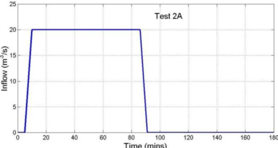
(11) Benchmarking of the Iber capabilities for 2D free surface flow modelling. 3. Test 2: Filling of floodplain depressions 3.1. Aims and description of the test The aim of this test is to verify the capability of the model to predict the extent of an inundation and the flood depth generated by a flow with low momentum over a complex topography. The geometry of this test case is a square domain with a side length of 2000 m. The topography (Figure 4) is a 4 x 4 matrix of 0.5 m deep depressions, obtained by multiplying sinusoids in the north to south and west to east directions. An underlying average slope of 1:1500 exists in the north-south direction, and of 1:3000 in the west-east direction. An inlet hydrograph is imposed at the north-west corner of the domain, along a 100 m long line running from north to south (Figure 4). The flow hydrograph at the inlet is shown in Figure 5. It starts from zero, rises to 20 m3/s, remains during 85 minutes with this value and then it falls to zero until the end of the simulation (48 hours). The total simulation time is 48 hours, in order to achieve an hydrostatic state. The initial condition of this test is a dry bed.. Figure 4. Test 2. Ground elevation with contour lines and inflow location for the test case 2. The localization of the control points 1, 4, 10 and 12 are also shown.. https://doi.org/10.17979/spudc.9788497497640. 11.

(12) Benchmarking of the Iber capabilities for 2D free surface flow modelling. Figure 5. Test 1. Flow hydrograph imposed at the inlet boundary.. 3.2. Numerical parameters and mesh The spatial domain is discretised with a structured mesh, with a grid resolution of 20 m in both directions. The total number of quadrilateral elements is therefore 10000 (100 x 100). The numerical schemes and parameters used in this test case are the following:     . Numerical schemes: Roe 1st order, Roe 2nd order, DHD, DHD basin Wet-dry threshold: 0.0001 m Time step: Adaptive with a CFL value between 0.35 and 0.9, depending on the numerical scheme Turbulence modelling: No Bed friction: Manning n= 0.03 (uniform in all the channel). 3.3. Results In order to verify the model outputs and to compare with some of the numerical models analysed in Defra´s report (TUFLOW, InfoWorks ICM and JFLOW+) the following variables are analysed:   . Total water volume at the end of the simulation Water level time series (with a time resolution of 300 s) at the centre of each depression. Water elevation time series at the centre of 4 depressions: Point 1, Point 4, Point 10 and point 12.. https://doi.org/10.17979/spudc.9788497497640. 12.

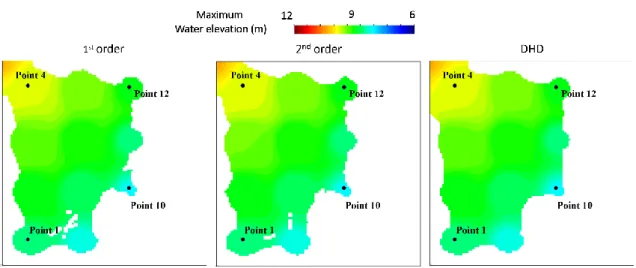
(13) Benchmarking of the Iber capabilities for 2D free surface flow modelling. Figure 6. 2D-map of the maximum water elevation obtained using Iber with three numerical schemes: Roe 1st order (left panel), Roe 2nd order (central panel) and DHD (right panel). Figure 6 shows the maximum value of water elevation obtained with Iber using the three numerical schemes. The differences between the results obtained with the three numerical schemes are negligible. The results show floods in 11 out of 16 floodplains with similar maximum water elevations at the end of the simulation.. Figure 7. Test 2. 2D-map of the water depth at the end of simulation using Iber with three numerical schemes: Roe 1st order (left panel), Roe 2nd order (central panel) and DHD (right panel).. Figure 8 shows the time series of the water elevation at the four control points (Point 4, Point 1, Point 12 and Point 10) obtained with Iber and the numerical codes TUFLOW, InfoWorks ICM and JFLOW+. At Point 4 (Figure7, upper-left panel) Iber performed very similar to the codes analysed in the Defra´s report for the three numerical schemes. All the time series obtained using Iber slightly overestimate the peak value obtained at Defra´s report with a maximum difference equal to 0.31 % (using the values of TUFLOW as reference) for the 2nd order scheme. The final value obtained using Iber is equal to the values obtained in Defra´s report. At Point 1 (Figure7, lower-left panel) some differences arise depending on the numerical scheme used with Iber although the final value obtained with Iber is similar to the final values obtained in the Defra´s report (maximum differences equal to 0.12 % obtained for the 2nd order scheme using the value obtained with TUFLOW as reference). Some discrepancies are also observed in the water arrival time. The results obtained in the Defra´s report show that the water arrives faster than with Iber using. https://doi.org/10.17979/spudc.9788497497640. 13.

(14) Benchmarking of the Iber capabilities for 2D free surface flow modelling. the DHD scheme, at the same time as Iber using the 2nd order scheme and later as Iber using the 1st order scheme. The behaviour at Point 12 (Figure7, upper-right panel) is similar to the observed at Point 1. Some differences in the water arrival time are observed depending on the numerical scheme used with Iber but at Point 12 there are higher differences in the final water elevation (0.54 % for the 1st order scheme) than at Point 1. At that point 12 Iber (using 1st and 2nd order numerical schemes) slightly overestimate the values of water elevation obtained in the Defra´s report. Using the DHD scheme the final values obtained with Iber are equivalent to those obtained with InfoWorks ICM and JFLOW +. At Point 10 (Figure7, lowerright panel) the water arrival times show a dependency on the numerical scheme: the faster one is the 1st order scheme and the slower one is the DHD scheme. The water arrival time obtained with the 2 nd order scheme is similar to the values obtained in the Defra´s report. The final water elevation obtained with Iber is greater than the values obtained in the Defra´s report (TUFLOW and InfoWorks ICM). The maximum difference is obtained with the DHD numerical scheme and is equal to 0.50 %. For all the analysed configurations the maximum difference between the maximum values of water elevation obtained with Iber and the values reported in the Defra´s report are less than 1 %.. Figure 8. Water elevation time series obtained with Iber using three numerical schemes (Roe 1st order, Roe 2nd order and DHD) and with TUFLOW, InfoWorks ICM and JFLOW+ at points 1, 4, 10 and 12.. https://doi.org/10.17979/spudc.9788497497640. 14.

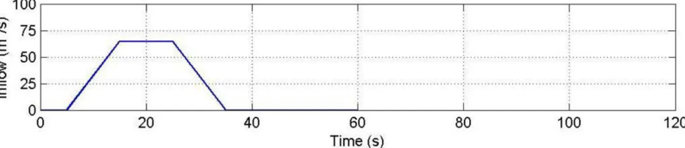
(15) Benchmarking of the Iber capabilities for 2D free surface flow modelling. 4. Test 3: Momentum conservation over a small obstruction 4.1. Aims and description of the test The aim of this test is to test the model capability to simulate shallow flows over an adverse slope obstruction. The model must be able to conserve momentum over the obstruction. This test case was originally proposed in order to differentiate between models that include inertia terms and those that neglect those terms in the shallow water equations to improve computational speed. Iber solves the complete shallow water equations (full inertia). The geometry of this test case is a one-dimensional 300 m long channel with the bed elevation shown in Figure 9. The topography has two depressions separated by a small hill. Since Iber is a 2D model, and in order to use the same spatial domain as in the original Defra’s report, the computational domain used in this test case is a 300 m x 100 m rectangle. However, the results are independent of the channel width (100 m). The boundary condition imposed at x = 0 m is a flow hydrograph, as shown in Figure 10. All other boundaries are closed and frictionless. The water volume of the inflow hydrograph is just enough to fill the first depression located at x = 150 m. However, due to the inertial terms, some water should pass over the obstruction to the second depression located at x = 250 m. The initial condition of this test is a dry bed. The total simulation time for this test is 15 minutes.. Figure 9. Test 3. Bed elevation of the channel and location of output points P1 and P2.. Figure 10. Test 3. Flow hydrograph imposed as boundary condition at x = 0 m (left boundary).. https://doi.org/10.17979/spudc.9788497497640. 15.

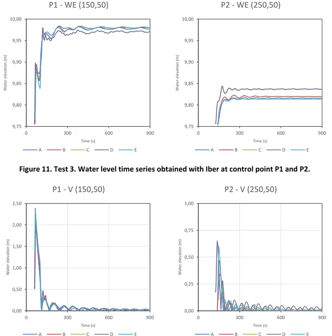
(16) Benchmarking of the Iber capabilities for 2D free surface flow modelling. 4.2. Numerical parameters and mesh The spatial domain is discretised with a structured mesh, with a grid resolution of 5 m in both directions. The total number of quadrilateral elements is therefore 1200 (60 x 20). This discretisation was chosen in order to use the same grid as the one used in the Defra’s report. However, since the geometry of the problem is 1D, the same results can be obtained with a single grid element of 100 m length in the transversal direction (i.e. with a mesh of 60 elements). In that case the CPU time would be 20 times lower. The numerical schemes and parameters used in this test case are the following:     . Numerical schemes: Roe 1st order, Roe 2nd order, DHD, DHD basin Wet-dry threshold: 0.0001 m Time step: Adaptive with a CFL value between 0.35 and 0.9, depending on the numerical scheme Turbulence modelling: No Bed friction: Manning n= 0.01 (uniform in all the channel). 4.3. Results In order to verify the model output and to compare the performance of different models, the Defra’s report analyses the following variables:  . Time series of velocity and water level (with a time resolution of 2 s) at the centre of the first depression (control point P1). Time series of water level (with a time resolution of 2 s) at the centre of the second depression (control point P2).. Model configuration resume: CASE. Model specifications Scheme st. Mesh. Time. CFL. Wet-Dry. Type. Elements. Seconds. A. Roe (1 ). 0.45. 0.0001. Structured. 1200. 8. B. Roe (2nd). 0.45. 0.0001. Structured. 1200. 8. C. DHD. 0.45. 0.0001. Structured. 1200. 9. D. DHD (Basin). 0.45. 0.0001. Structured. 1200. 9. 0.45. 0.0001. Structured. 7500. 40. E. nd. Roe (2 ). In general, the simulation time was similar in all cases analysed in exception of the case E, whose number of elements was 4-times higher, thus the computational time was 4-times higher too. In all cases the water reach and overtops the hill, so a wave travel through the second depression (all the numerical schemes implemented in Iber solve the full-SWE, with inertia terms). The water evolution at point P1 presents slightly differences at the arrival time of the wave front (less than 4 s in all cases). First and second order numerical schemes solutions were very similar, but some differences were presented in comparison with the DHD and DHD basin numerical schemes. Both reproduced suitable the phenomenon, but some oscillations and a slightly underestimation of the water level were occurred since t = 120 s. In terms of velocity, the differences are depreciable. The same oscillations were presented in the DHD and DHD basin solutions. At point P2 the water evolution was very similar in exception of DHD and DHD basin numerical schemes, in which the water level was higher than the other solutions. This phenomenon is due to different treatment of the free surface elevation that provided higher inertial energy and, thus, higher volume of. https://doi.org/10.17979/spudc.9788497497640. 16.

(17) Benchmarking of the Iber capabilities for 2D free surface flow modelling. water overtopped the obstacle. The free surface became smoother faster with the 1st order scheme than 2nd order. All simulations finished without numerical stability problems. The CFL and wet-dry limit values chosen had influence only in the arrival time of the wet-front and the volume.. P1 - WE (150,50). P2 - WE (250,50). 9,95. 9,95 Water elevation (m). 10,00. Water elevation (m). 10,00. 9,90. 9,85. 9,80. 9,90. 9,85. 9,80. 9,75. 9,75 0. 300. 600. 900. 0. 300. Time (s). A. B. 600. 900. Time (s). C. D. E. A. B. C. D. E. Figure 11. Test 3. Water level time series obtained with Iber at control point P1 and P2.. P1 - V (150,50). P2 - V (250,50). 2,50. 1,00. 2,00 Water elevation (m). Water elevation (m). 0,75 1,50. 1,00. 0,50. 0,25 0,50. 0,00. 0,00 0. 300. 600. 900. 0. 300. Time (s). A. B. C. 600. 900. Time (s). D. E. A. B. C. D. E. Figure 12. Test 3. Velocity time series obtained with Iber at control point P1 and P2. https://doi.org/10.17979/spudc.9788497497640. 17.

(18) Benchmarking of the Iber capabilities for 2D free surface flow modelling. 5. Test 4: Speed of flood propagation over an extended floodplain 5.1. Aims and description of the test The aim of this test is to verify the model capability to simulate the speed of propagation of a flood wave over a dry domain. This test tries to replicate a simplified failure of an embankment. The prediction of velocities at the leading edge of the flood front is also analysed. The geometry of this test case is a 1000 m x 2000 m rectangle (Figure 13). The bed elevation is horizontal, with an elevation of z = 0 m. The inlet boundary condition is a flow hydrograph imposed along a 20 m long line running from north to south and centred at the location x = 0 m, y = 1000 m (middle of the left boundary). The hydrograph starts from zero, rises linearly to a peak value of 20 m3/s during the first hour, it remains with this value during 3 hours and then it falls again to zero in 1 hour (Figure 14). All the other boundaries are closed and frictionless. The initial condition of this test is a dry bed. The total simulation time for this test is 5 hours.. Figure 13. Test 4. Spatial domain and location of the control points.. Figure 14. Test 4. Flow hydrograph imposed at the inlet boundary. https://doi.org/10.17979/spudc.9788497497640. 18.

(19) Benchmarking of the Iber capabilities for 2D free surface flow modelling. 5.2. Numerical parameters and mesh The spatial domain is discretised with a structured mesh, with a grid resolution of 5 m in both directions. The total number of quadrilateral elements is therefore 80000 (200 x 400). The numerical schemes and parameters used in this test case are the following:     . Numerical schemes: Roe 1st order, Roe 2nd order, DHD, DHD basin Wet-dry threshold: 0.0001 m Time step: Adaptive with a CFL value between 0.35 and 0.9, depending on the numerical scheme Turbulence modelling: No Bed friction: Manning n= 0.05 (uniform in all the channel). 5.3. Results In order to verify the model output and to compare the performance of different models, the Defra’s report analyses the following results:   . 2D spatial maps of water depth at the following times: 0.5, 1, 2, 3, 4 hours. 2D spatial maps of water velocity modulus at the following times: 0.5, 1, 2, 3, 4 hours. Time series of water elevation and velocity (with a time resolution of 20 s) at the six control points shown in Figure 13.. Model configuration resume: CASE. Model specifications Scheme st. Mesh. CFL. Wet-Dry. Type. Time. Elements HH:MM:SS. A. Roe (1 ). 0.45. 0.0001. Structured. 80000. 0:27:46. B. Roe (2nd). 0.45. 0.0001. Structured. 80000. 0:34:09. C. DHD. 0.45. 0.0001. Structured. 80000. 0:20:13. D. DHD (Basin). 0.45. 0.0001. Structured. 80000. 0:22:08. All tests done remark the adjustment of the different numerical schemes implemented in Iber. Only small differences were presented at point P1, especially in the 1st order model where the water velocity was always higher than the other simulations. However, the water elevation was clearly similar in all simulations. The arrival of the water front was always lower for models computed with DHD’s schemes. As expected, the velocity field of the DHD’s schemes was smoother than the other schemes evaluated. In the other hand, 2nd order scheme reached more than 5 minutes of delay in the water front at the farther point (P6) versus the 1st order scheme, but these differences became negligible few seconds after in water elevation and velocity terms. In terms of computation time, it is remarkable the speed-up of the DHD’s schemes versus 1st and 2nd order numerical schemes, between 1.3 and 1.7 times faster.. https://doi.org/10.17979/spudc.9788497497640. 19.

(20) Benchmarking of the Iber capabilities for 2D free surface flow modelling. Case. A. B. C. WE. Velocity. Figure 15. Test 4. Water elevation and velocity maps at time t = 0.5 h.. https://doi.org/10.17979/spudc.9788497497640. 20.

(21) Benchmarking of the Iber capabilities for 2D free surface flow modelling. P3 - WE (200,1000). 0,40. 0,40. 0,30. 0,30 Water elevation (m). Water elevation (m). P1 - WE (50,1000). 0,20. 0,10. 0,20. 0,10. 0,00. 0,00 0. 3600. 7200. 10800. 14400. 18000. 0. 3600. 7200. Time (s). A. B. C. D. E. A. P5 - WE (400,1000). 14400. 18000. B. C. D. E. P6 - WE (300,1300). 0,40. 0,40. 0,30. 0,30 Water elevation (m). Water elevation (m). 10800 Time (s). 0,20. 0,10. 0,20. 0,10. 0,00. 0,00 0. 3600. 7200. 10800. 14400. 18000. 0. 3600. 7200. Time (s). A. B. C. 10800. 14400. 18000. Time (s). D. E. A. B. C. D. E. Figure 16. Test 4. Evolution of the water elevation at P1, P3, P5 and P6 points.. https://doi.org/10.17979/spudc.9788497497640. 21.

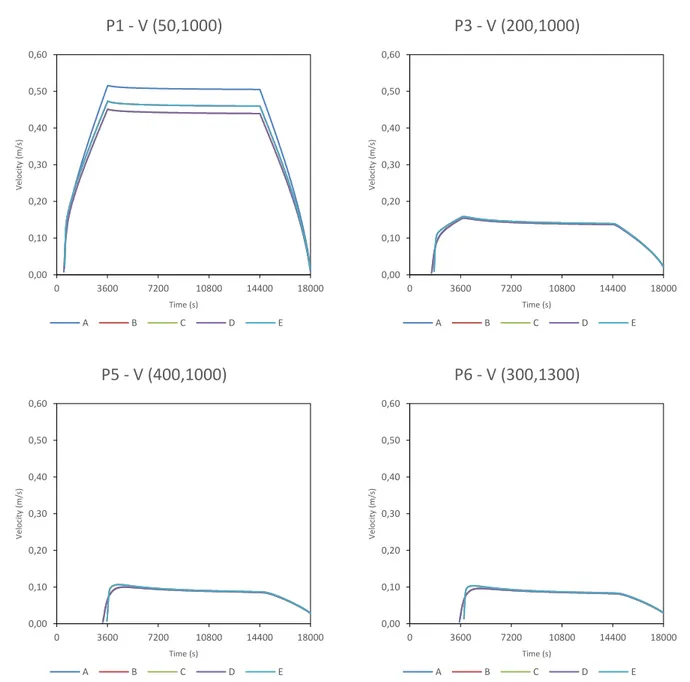
(22) Benchmarking of the Iber capabilities for 2D free surface flow modelling. P3 - V (200,1000). 0,60. 0,60. 0,50. 0,50. 0,40. 0,40 Velocity (m/s). Velocity (m/s). P1 - V (50,1000). 0,30. 0,30. 0,20. 0,20. 0,10. 0,10. 0,00. 0,00 0. 3600. 7200. 10800. 14400. 18000. 0. 3600. 7200. Time (s). A. B. C. D. E. A. P5 - V (400,1000). 14400. 18000. B. C. D. E. P6 - V (300,1300). 0,60. 0,60. 0,50. 0,50. 0,40. 0,40 Velocity (m/s). Velocity (m/s). 10800 Time (s). 0,30. 0,30. 0,20. 0,20. 0,10. 0,10. 0,00. 0,00 0. 3600. 7200. 10800. 14400. 18000. 0. 3600. 7200. Time (s). A. B. C. 10800. 14400. 18000. Time (s). D. E. A. B. C. D. E. Figure 17. Test 4. Evolution of the water velocity at P1, P3, P5 and P6 points.. https://doi.org/10.17979/spudc.9788497497640. 22.

(23) Benchmarking of the Iber capabilities for 2D free surface flow modelling. 6. Test 5: Valley flooding 6.1. Aims and description of the test The aim of this test is to verify the model capability to simulate flood inundation at the valley scale arising from a dam failure. The test replicates the propagation of a flood wave generated by the failure of a dam. The DEM of the valley is shown in Figure 18. The length of the valley is approximately 17 km, with an average width of 0.8 km. The upstream boundary condition is a flow hydrograph imposed along a 260 m long line, with a peak discharge of 3000 m3/s (Figure 19). All the other boundaries are closed and frictionless. The initial condition of this test is a dry bed. The total simulation time for this test is 30 hours.. Figure 18. Test 5. Topography of the valley and location of control points: Point 1, Point 3, Point 4, Point 5 and Point 7.. Figure 19. Test 5. Flow hydrograph imposed at the upstream boundary.. https://doi.org/10.17979/spudc.9788497497640. 23.

(24) Benchmarking of the Iber capabilities for 2D free surface flow modelling. 6.2. Numerical parameters and mesh The spatial domain is discretised with an unstructured mesh, with a mesh resolution of 75 m. The total number of triangular mesh elements is 7594. The average element size is ≈2500 m2.The numerical schemes and parameters used in this test case are the following:     . Numerical schemes: Roe 1st order, Roe 2nd order, DHD, DHD basin Wet-dry threshold: 0.0001 m Time step: Adaptive with a CFL value between 0.35 and 0.9, depending on the numerical scheme Turbulence modelling: No Bed friction: Manning n= 0.04 (uniform in all the channel). 6.3. Results In order to verify the model outputs and to compare with some of the numerical models analysed in Defra´s report (TUFLOW, InfoWorks ICM and JFLOW+) the following variables are analysed:    . 2D spatial map of maximum water levels during the simulation. 2D spatial map of maximum water depths during the simulation. 2D spatial map of maximum water velocities (modulus) during the simulation. Time series of water elevation and velocity (with a time resolution of 60 s) at the seven control points shown in Figure 18.. Figure 20 shows the water depth at the end of the simulations obtained with Iber using the three numerical schemes. The differences between the results obtained with the three numerical schemes are negligible. The results obtained with DHD scheme shows a wet area slightly greater than the wet area obtained using the 1st and 2nd order numerical schemes. Figure 8 shows the results obtained with most of the models analysed in the Defra´s reports. The results obtained with Iber are similar to those obtained with the numerical codes analysed in the Defra´s report.. Figure 20. 2D spatial map of water depth at the end of the simulation obtained with Iber using three numerical schemes: Roe 1st order (left panel), Roe 2nd order (central panel) and DHD (right panel). Figure 21 shows the time series of water elevation at points 1, 3, 5 and 7 using Iber and three of the numerical codes analysed in the Defra´s report: TUFLOW, InfoWorks ICM and JFLOW+. The results obtained with Iber are similar to those showed in the Defra´s report.. https://doi.org/10.17979/spudc.9788497497640. 24.

(25) Benchmarking of the Iber capabilities for 2D free surface flow modelling. Figure 21. Water elevation time series obtained with Iber using three numerical schemes, TUFLOW, InfoWorks ICM and JFLOW+ at points 1, 3, 5 and 7.. Figure 22 shows the time series of velocity at points 1, 3, 4 and 7 using Iber and three of the numerical codes analysed in the Defra´s report: TUFLOW, InfoWorks ICM and JFLOW+. The discrepancies between the results obtained with Iber and the numerical codes analysed in the Defra´s report are greater than those observed in the time series of water elevation (see Figure 20). The water arrival times at the four control points obtained with Iber are similar to those obtained with TUFLOW, InfoWorks ICM and JFLOW+. The peak and final values of velocity obtained with Iber are similar to the peak values obtained with TUFLOW, InfoWorks ICM and JFLOW+. Only the peak value obtained at Point 1 using TUFLOW and final values at Point 3 obtained with TUFLOW, InfoWorks ICM and JFLOW + shows a high discrepancy to the values obtained with Iber.. https://doi.org/10.17979/spudc.9788497497640. 25.

(26) Benchmarking of the Iber capabilities for 2D free surface flow modelling. Figure 22. Velocity time series obtained with Iber using three numerical schemes, TUFLOW, InfoWorks ICM and JFLOW+ at points 1, 3, 4 and 7.. https://doi.org/10.17979/spudc.9788497497640. 26.

(27) Benchmarking of the Iber capabilities for 2D free surface flow modelling. 7. Test 6: Dambreak 7.1. Aims and description of the test The aim of this test is to verify the model capability to simulate transcritical flow, hydraulic jumps and wakes behind obstructions. The test case corresponds to the laboratory dambreak presented in Soares-Frazão and Zech (2002). It is a simplified dambreak in a laboratory channel, with a single building located downstream from the dam (Figure 23). The initial condition is a uniform water elevation of 0.4 m upstream from the dam and a uniform water elevation of 0.02 m downstream from the dam. At all the boundaries there are vertical walls. Defra proposed two variants of this case. Test 6A has the original dimensions presented in Soares-Frazão and Zech (2002), while in Test 6B all physical dimensions (include the initial water levels) are multiplied by 20 to obtain physical dimensions more similar to those encountered in practical applications. For the purpose of this document, the study case was modified limiting the domain to 30 m downstream and imposing an outlet condition in critical/supercritical flow. The geometry was built following the scheme of the Figure 23. The total simulation time in this case is 30 seconds for the Test 6A and 30 min for the Test 6B.. Figure 23. Test 6. Geometry and dimensions for Test 6A.. https://doi.org/10.17979/spudc.9788497497640. 27.

(28) Benchmarking of the Iber capabilities for 2D free surface flow modelling. 7.2. Numerical parameters and mesh The spatial domain is discretised with a mixt mesh (triangular and quadrilateral shapes), with a mesh resolution of 0.1 m side-size in Test 6A and 2 m side-size in Test 6B. The total number of elements is approximately 25000 in both cases. The numerical schemes and parameters used in this test case are the following:     . Numerical schemes: Roe 1st order, Roe 2nd order, DHD, DHD basin Wet-dry threshold: 0.0001 m Time step: Adaptive with a CFL value between 0.35 and 0.9, depending on the numerical scheme Turbulence modelling: No Bed friction: Manning n= 0.01 in Test 6A and n= 0.05 in Test 6B (in both cases uniform in all the channel). 7.3. Results In order to verify the model output and to compare the performance of different models, the Defra’s report analyses the following results: Test 6A:    . 2D spatial map of maximum water levels reached during the simulation. 2D spatial map of maximum water velocities (modulus) reached during the simulation. 2D spatial maps of water levels at times 1, 2, 3, 4, 5, 10, 15, 20, 25 and 30 seconds. Time series of water elevation and velocity (with a time resolution of 0.1 s) at the six control points shown in Figure 23.. Test 6B:    . 2D spatial map of maximum water levels reached during the simulation. 2D spatial map of maximum water velocities (modulus) reached during the simulation. 2D spatial maps of water levels at times 0.5, 1, 2, 3, 4, 5 and 10 minutes. Time series of water elevation and velocity (with a time resolution of 1 s) at the six control points shown in Figure 23.. Test 6A Model configuration resume: CASE. Model specifications Scheme st. Mesh. CFL. Wet-Dry. Type. Time. Elements HH:MM:SS. A. Roe (1 ). 0.45. 0.0001. Mixt. 24550. 0:01:47. B. Roe (2nd). 0.45. 0.0001. Mixt. 24550. 0:02:06. C. DHD. 0.45. 0.0001. Mixt. 24550. 0:01:36. D. DHD (Basin). 0.45. 0.0001. Mixt. 24550. 0:01:37. 0.45. 0.0001. Mixt. 95722. 0:07:50. E. nd. Roe (2 ). The numerical results of this study case were compared with experimental data (Soares-Frazão and Zech, 2002). The flume measurements has oscillations and, as expected, numerical results cannot reproduce it due nature of the model (2D model versus 3D and bi-phase air-water behaviour) and the spatial and temporal discretization used. For this reason, the results analysis is focused in the differences of the different numerical schemes and the general adjustment (location of the hydraulic jump and shock wave). https://doi.org/10.17979/spudc.9788497497640. 28.

(29) Benchmarking of the Iber capabilities for 2D free surface flow modelling. Some remarkable differences were presented at point G2 from 15 s of the simulation, but all models well captured the hydraulic jump. At point G3 all models slightly overestimate the water elevation, but in general the shock wave was well represented in time and in space. In terms of velocity, a general underestimation was observed in all control points, being the configuration E the best fit, especially at point G5 (Figure 25). For these models configuration, the best adjustment was obtained by 2nd order numerical scheme (E). DHD’s models smoothed the solution, and the was not differences between both.. G3 - WE (4,1.15). 0,20. 0,20. 0,15. 0,15 Water elevation (m). Water elevation (m). G1 - WE (2.65,1.15). 0,10. 0,05. 0,10. 0,05. 0,00. 0,00 0. 10. 20. 30. 0. 10. 20. Time (s). A. B. C. D. E. Exp. A. G4 - WE (4,-0.8). B. C. D. E. Exp. G5 - WE (5.2,0.3). 0,20. 0,20. 0,15. 0,15 Water elevation (m). Water elevation (m). 30. Time (s). 0,10. 0,05. 0,10. 0,05. 0,00. 0,00 0. 10. 20. 30. 0. 10. 20. Time (s). A. B. C. 30. Time (s). D. E. Exp. A. B. C. D. E. Exp. Figure 24. Test 6A. Time series of the water elevation at G1, G3, G4 and G5 control points.. Very similar results are shown in the Figure 26, in which the velocity field is represented. The hydraulic jump is sharper with the 1st scheme than DHD’s schemes due the simplifications done in the upwind discretization of the momentum and mass fluxes.. https://doi.org/10.17979/spudc.9788497497640. 29.

(30) Benchmarking of the Iber capabilities for 2D free surface flow modelling. G1 - V (2.65,1.15). G3 - V (4,1.15). 2,50. 2,25 2,00. 2,00. 1,75. Velocity (m/s). Velocity (m/s). 1,50 1,50. 1,00. 1,25 1,00 0,75 0,50. 0,50. 0,25 0,00. 0,00 0. 10. 20. 30. 0. 10. 20. Time (s). A. B. C. 30. Time (s). D. E. Exp. A. B. G4 - V (4,-0.8). C. D. E. Exp. G5 - V (5.2,0.3). 2,25. 1,50. 2,00 1,25 1,75 1,00 Velocity (m/s). Velocity (m/s). 1,50 1,25 1,00 0,75. 0,75. 0,50. 0,50 0,25 0,25 0,00. 0,00 0. 10. 20. 30. 0. 10. 20. Time (s). A. B. C. 30. Time (s). D. E. Exp. A. B. C. D. E. Exp. Figure 25. Test 6A. Time series of the water elevation at G1, G3, G4 and G5 control points.. https://doi.org/10.17979/spudc.9788497497640. 30.

(31) Benchmarking of the Iber capabilities for 2D free surface flow modelling. Figure 26. Test 6A. Velocity field comparison between 1st and DHD schemes 5 s after the gate opening.. Test 6B Model configuration resume: CASE. Model specifications Scheme st. Mesh. Time. CFL. Wet-Dry. Type. Elements HH:MM:SS. A. Roe (1 ). 0.45. 0.0001. Mixt. 24550. 0:03:41. B. Roe (2nd). 0.45. 0.0001. Mixt. 24550. 0:04:28. C. DHD. 0.45. 0.0001. Mixt. 24550. 0:03:05. D. DHD (Basin). 0.45. 0.0001. Mixt. 24550. 0:03:44. E. Roe (2nd). 0.45. 0.0001. Mixt. 95664. 0:13:01. In this case, as a part of the DEFRA’s report, all dimensions are multiplied by 20. No experimental data exists, thus only numerical comparison was done between the different numerical schemes implemented in Iber. All models predict the peak of the water level and velocity downstream of the gate with a good agreement. Small differences are presented for the 2nd order models, where the oscillations on the water surface occurred. Thus, the case E (2nd order and 4-times more elements) allowed reducing this phenomenon, especially at point G6. The hydraulic jump was spatially bigger than Test 6A. The shock waves are also well captured due no important differences were presented in the peaks of the water elevation and velocities.. https://doi.org/10.17979/spudc.9788497497640. 31.

(32) Benchmarking of the Iber capabilities for 2D free surface flow modelling. G3 - WE (80,23). 4,00. 4,00. 3,00. 3,00 Water elevation (m). Water elevation (m). G1 - WE (53,23). 2,00. 1,00. 2,00. 1,00. 0,00. 0,00 0. 200. 400. 600. 0. 200. Time (s). A. B. C. D. E. A. G4 - WE (80,-16). 600. B. C. D. E. G5 - WE (104,6). 4,00. 4,00. 3,00. 3,00 Water elevation (m). Water elevation (m). 400 Time (s). 2,00. 1,00. 2,00. 1,00. 0,00. 0,00 0. 200. 400. 600. 0. 200. Time (s). A. B. C. 400. 600. Time (s). D. E. A. B. C. D. E. Figure 27. Test 6B. Time series of the water elevation at G1, G3, G4 and G5 control points.. https://doi.org/10.17979/spudc.9788497497640. 32.

(33) Benchmarking of the Iber capabilities for 2D free surface flow modelling. G3 - V (80,23). 5,00. 5,00. 4,00. 4,00. 3,00. 3,00. Velocity (m/s). Velocity (m/s). G1 - V (53,23). 2,00. 1,00. 2,00. 1,00. 0,00. 0,00 0. 200. 400. 600. 0. 200. Time (s). A. B. C. 400. 600. Time (s). D. E. A. G4 - V (80,-16). B. C. D. E. G5 - V (104,6). 5,00. 4,00. 4,00. 3,00. Velocity (m/s). Velocity (m/s). 3,00. 2,00. 2,00. 1,00 1,00. 0,00. 0,00 0. 200. 400. 600. 0. 200. Time (s). A. B. C. 400. 600. Time (s). D. E. A. B. C. D. E. Figure 28. Test 6B. Time series of the water elevation at G1, G3, G4 and G5 control points.. https://doi.org/10.17979/spudc.9788497497640. 33.

(34) Benchmarking of the Iber capabilities for 2D free surface flow modelling. Figure 29. Test 6A. Velocity field comparison between 1st and DHD schemes 5 s after the gate opening.. https://doi.org/10.17979/spudc.9788497497640. 34.

(35) Benchmarking of the Iber capabilities for 2D free surface flow modelling. 8. Test 7: Rainfall and point source surface flow in urban areas 8.1. Aims and description of the test The aim of this test is to verify the model capability to simulate overland flow originating from a point source and from rainfall inputs directly applied to the model grid. The spatial domain is an urban area of approximately 400 m x 960 m (Figure 30). The topography is defined from a DTM with a spatial resolution of 0.5 m. Buildings and vegetation are not included in the DTM and should be ignored in the simulation. The two sources of flooding are the following:  . An inflow discharge imposed as a point source at the location shown in Figure 30. The discharge time series is shown in Figure 31. A spatially uniform rainfall defined by the hyetograph shown in Figure 32.. All the boundaries of the spatial domain are considered as closed frictionless walls. The initial condition of this test is a dry bed. The total simulation time for this test is 5 hours.. Figure 30. Test 8. Topography, point source and control points.. https://doi.org/10.17979/spudc.9788497497640. 35.

(36) Benchmarking of the Iber capabilities for 2D free surface flow modelling. Figure 31. Test 8. Flow hydrograph imposed at the upstream boundary.. Figure 32. Test 8. Rain hyetograph imposed directly at the model grid.. 8.2. Numerical parameters and mesh The spatial domain is discretised with a structured mesh, with a grid resolution of 2 m. The total number of quadrilateral elements is 95720. The numerical schemes and parameters used in this test case are the following:     . Numerical schemes: Roe 1st order, Roe 2nd order and DHD Wet-dry threshold: 0.0001 m Time step: Adaptive with a CFL value of 0.5 Turbulence modelling: No Bed friction: Manning n= 0.02 in roads and pavements, and n = 0.05 elsewhere. https://doi.org/10.17979/spudc.9788497497640. 36.

(37) Benchmarking of the Iber capabilities for 2D free surface flow modelling. 8.3. Results In order to verify the model output and to compare the performance of different models, the Defra’s report analyses the following results:   . 2D spatial map of maximum water levels reached during the simulation. 2D spatial map of maximum water depths reached during the simulation. Time series of water elevation and velocity (with a time resolution of 30 s) at the 9 control points shown in Figure 30.. Figure 33. Temporal evolution of the water velocity at points P2 and P6.. https://doi.org/10.17979/spudc.9788497497640. 37.

(38) Benchmarking of the Iber capabilities for 2D free surface flow modelling. Figure 34. Temporal evolutions of the water elevation at points P1, P2 and P3. .. https://doi.org/10.17979/spudc.9788497497640. 38.

(39) Benchmarking of the Iber capabilities for 2D free surface flow modelling. Regarding the computed water levels, the Iber model correctly reproduces the double peak observed in all the other models, caused by the intense rainfall (first peak) and the inflow discharge (second peak). Also, due to the short travelling times, the timings of these peaks are very similar to the ones reported by other models. In terms of the value of the maximum water depth, similar results are obtained by all the models, within a range of only a few centimetres. The peak water level caused by the rain event is slightly higher in the computations performed using the Iber model. This is probably explained by the low wetdry threshold, which increases the mobilized rainfall-runoff volumes. By the end of the simulation, the water depth varies from one model to another. This is caused by the different approaches used to process the topography, which suggests that finer spatial discretization are recommended in urban flood studies. In the computations performed using the Iber model, very similar results are obtained with the first and second order extension of the Roe scheme. The water depths computed using the DHD scheme are slightly different, although at the end of the simulation these differences become nearly negligible. In terms of the computed water velocities, the differences observed between the analysed models are higher than the ones observed for the water depths. During the peak caused by the inflow discharge, the water velocity varies importantly depending on the considered model. This variation is higher at points as P6, located near a wet-dry front. At these points, the different treatment of the wet-dry front performed by each model results in different velocities. The results of the computations performed using the Iber model show that similar velocities are obtained using either the first or the second order scheme of Roe, while higher differences are observed when the DHD scheme is used. However, for all the cases, the results of the Iber model are in close agreement with the ones obtained by other models.. https://doi.org/10.17979/spudc.9788497497640. 39.

(40) Benchmarking of the Iber capabilities for 2D free surface flow modelling. 9. Test 8: Overland flow in a four-branch junction 9.1. Aims and description of the test The aim of this test is to verify the model capability to simulate overland flow under the conditions that can be found in urban areas. Most specifically, it tests the ability of the model to solve accurately shallow flow under steady supercritical flow conditions including an oblique hydraulic jump. The spatial domain is a 90o four-branch open-channel junction and it tries to replicate a street junction. The geometry and dimensions of the modelled domain are shown in Figure 35. The slope of the channels aligned with the x- and y-axis are respectively 0.01 and 0.02 m/m, while the junction itself is a horizontal square 1.5 m wide. This configuration was tested in the laboratory. A thorough description of the setup and experimental methodology can be found in Nania et al. (2011). Experimental water depth maps are available for the following flow conditions:   . Qin,x = 0.0429 m3/s Qin,y = 0.100 m3/s Supercritical flow at both channel outlets. All the other boundaries are closed walls. The bed surface is made of concrete, with an estimated Manning coefficient of 0.016. Under these experimental flow conditions the flow is subcritical in the inlet aligned with the x-axis and supercritical in the inlet aligned with the y-axis, and an oblique hydraulic jump is formed in the junction. Downstream the junction the flow returns to supercritical conditions in both channels. The Froude numbers varies from 0.2 to 4 inside the domain. The model is run until steady flow conditions are reached. The steady state water depth maps will be compared with the experimental laboratory data. The initial condition of this test is a dry bed, although any other condition can be used in the model since only the steady state will be used to analyse model performance.. Figure 35. Test 9. Topography, point source and control points.. https://doi.org/10.17979/spudc.9788497497640. 40.

(41) Benchmarking of the Iber capabilities for 2D free surface flow modelling. 9.2. Numerical parameters and mesh The spatial domain is discretised with an structured mesh, with a grid resolution of 0.05 m-squares in the upper part (the firsts 4.5 m of each branch) and a grid of 0.1x0.05 m-quadrilateral elements in the lower part (1.5 m downstream of the junction). This geometrical configuration provides a mesh of 6600 elements. An extra simulation (case E) was done using 4-times more elements. The numerical schemes and parameters used in this test case are the following:     . Numerical schemes: Roe 1st order, Roe 2nd order, DHD, DHD basin Wet-dry threshold: 0.0001 m Time step: Adaptive with a CFL value between 0.35 and 0.9, depending on the numerical scheme Turbulence modelling: No Bed friction: Manning n= 0.016. 9.3. Results In order to verify the model output and to compare the performance of different models, the following results will be compared with the available experimental data (location of the axis shown in Figure 26):    . 2D spatial map of water depth at the steady state, as shown in Figure 35. Profile along the axis x=0.675m of the y-velocity component (Vy) Profile along the axis y=0.675m of the x-velocity component (Vx) Validation of the outlet discharges for different hydraulic conditions. Model configuration resume: CASE. Model specifications Scheme st. Mesh. CFL. Wet-Dry. Type. Time. Elements HH:MM:SS. A. Roe (1 ). 0.45. 0.0001. Mixt. 6600. 0:00:24. B. Roe (2nd). 0.45. 0.0001. Mixt. 6600. 0:00:37. C. DHD. 0.45. 0.0001. Mixt. 6600. 0:00:17. D. DHD (Basin). 0.45. 0.0001. Mixt. 6600. 0:00:16. 0.45. 0.0001. Mixt. 26400. 0:02:25. E. nd. Roe (2 ). The 1st and 2nd order schemes give a sharper and accurate definition of the hydraulic jump than the DHD scheme, which in general predicts a smoother variation of the free surface elevation and velocity, as shown in the longitudinal profiles represented in Figure 37. Despite these differences in the results obtained with all schemes, the DHD predicts correctly the position and strength of the hydraulic jump, and the global agreement with the experimental data is very satisfactory for both schemes, as shown in Figure 36. As expected, using a dense grid (case E) the results were more precise. The hydraulic jump had a better definition, also the cross-waves downstream of the junction.. https://doi.org/10.17979/spudc.9788497497640. 41.

(42) Benchmarking of the Iber capabilities for 2D free surface flow modelling. Roe 1st (A). Roe 2nd (B). DHD (D). Roe 2nd (E). Figure 36. Test 9. Water depth maps computed with the different numerical schemes.. https://doi.org/10.17979/spudc.9788497497640. 42.

(43) Benchmarking of the Iber capabilities for 2D free surface flow modelling. WE (y = 0.675 m). Vx (y = 0.675 m). 0,12. 1,80 1,60. 0,10. 0,08. 1,20 X-Velocity (m/s). Water elevation (m). 1,40. 0,06. 0,04. 1,00 0,80 0,60 0,40. 0,02 0,20 0,00. 0,00 -2. 0. 2. 4. 6. -1,5. 0,5. 2,5. X (m). A. B. C. D. E. Exp. A. WE (x = 0.675 m). 6,5. B. C. D. E. Exp. Vy (x = 0.675 m). 0,14. -0,40. 0,12. -0,60. 0,10. -0,80 Y-Velocity (m/s). Water elevation (m). 4,5. X (m). 0,08 0,06. -1,00 -1,20. 0,04. -1,40. 0,02. -1,60. 0,00. -1,80 -5. -3. -1. 1. 3. -5. -3. -1. Y (m). A. B. C. 1. 3. Y (m). D. E. Exp. A. B. C. D. E. Exp. Figure 37. Test 9. Experimental and numerical profiles of water depth and velocity. Water depth at y=0.675m (top-left), Vx at y=0.675 (top-right), water depth at x=0.675m (bottom-left), and Vy at x=0.675 (bottom-right). Additional models were calculated using the same geometry but changing the discharges and the slopes of the inlet/outlet branches. The discharges varied from 0.0152 to 0.1136 m 3/s in the Y-axis and from 0.021 to 0.1094 m3/s in the X-axis. The slopes were maintained constant upstream and downstream of the junction with values from 1 to 2 %. All of these cases were run with 1st order scheme using an unstructured mesh around 6000 elements. As shown in Figure 38, the numerical results had very high adjustment to the experimental data. The mean error was less than 2.5 % (absolute value) and the R-squared value was up to 0.99 for all cases. In conclusion, the model predicts accurately the hydraulic behaviour capturing the hydraulic jump (transcritical flow), the cross-waves (supercritical flow) and satisfying the mass conservation equation.. https://doi.org/10.17979/spudc.9788497497640. 43.

(44) Benchmarking of the Iber capabilities for 2D free surface flow modelling. Qx. Qy. 120. 120. 1%-1% R2 = 0.9962. 2. 1%-1% R = 0.9952 100. 2%-2% R2 = 0.9975. 1%-2% R2 = 0.9975 2%-2% R2 = 0.9992. 80 Experimantal. 80 Experimantal. 100. 1%-2% R2 = 0.9958. 60. 60. 40. 40. 20. 20. 0. 0 0. 20. 40. 60. 80. Numerical. 100. 120. 0. 20. 40. 60. 80. 100. 120. Numerical. Figure 38. Test 9. Comparison between experimental and numerical outlet discharges from different slopes of the branches. A more detailed description of this test case can be found in Bladé (2005) and Nanía Escobar (1999).. https://doi.org/10.17979/spudc.9788497497640. 44.

(45) Benchmarking of the Iber capabilities for 2D free surface flow modelling. 10. Test 9: Rainfall-runoff in a three-slope 1D channel 10.1. Aims and description of the test The aim of this test is to validate the model capability to simulate the generation of surface runoff from rainfall data and its propagation under supercritical flow conditions. The experimental results presented by Iwagaki (1955) in a 24 m long laboratory flume made of very smooth aluminium are used to compare with the numerical predictions. The available experimental data are the hydrographs measured at the flume outlet for three different rainfall conditions. The spatial domain is a 24 long one-dimensional flume with three reaches of equal length but different slope: 0.020, 0.015 and 0.010 respectively from upstream to downstream (Figure 39). The rainfall intensity over the upper, middle and lower reaches is respectively 3890, 2300 and 2880 mm/h. Notice that these are extremely large intensities, and physically impossible in a real application. They have been used here since they are the ones used by Iwagaki (1955) and serve to test the model under extreme conditions. The duration of the rainfall for three different experimental conditions is 10, 20 and 30 s. These flow conditions produce rapidly varying flow, since the highest rainfall intensity occurs in the upstream steepest reach, while the lowest rainfall intensity and bed slope are those of the downstream reach. Since the case is one-dimensional, the results are independent of the channel width. The only boundary condition is the open downstream outlet. The flume lateral boundaries are considered as closed frictionless walls. The initial condition of this test is a dry bed. Since the bed material of the flume is aluminium, there are no infiltration losses and all the rainfall contributes to generate surface runoff. The total simulation time for all the test is 60 s and the duration of the rainfall is 10, 20 and 30 s for test 1, 2 and 3 respectively as it defined above.. Figure 39. Test 10. Longitudinal profile of the flume.. 10.2. Numerical parameters and mesh The spatial domain is discretised with a structured mesh, with a grid resolution of 0.1 m. Since the results are independent of the channel width, a single grid element was used in the y-direction. The total number of quadrilateral elements is therefore 240.. https://doi.org/10.17979/spudc.9788497497640. 45.

(46) Benchmarking of the Iber capabilities for 2D free surface flow modelling. The numerical results of this case are very sensitive to the Manning coefficient and therefore, its value can be calibrated as a function of the numerical model or scheme used. Nonetheless, the same value of the Manning coefficient must be used to model the three hyetographs. The numerical schemes and parameters used in this test case are the following:     . Numerical schemes: Roe 1st order, Roe 2nd order, DHD, DHD basin Wet-dry threshold: 0.0001 m Time step: Adaptive with a CFL value between 0.35 and 0.9, depending on the numerical scheme Turbulence modelling: No Bed friction: Manning coefficient (uniform in all the flume) to be calibrated for each numerical scheme. The same value of the Manning coefficient must be used for the three experimental conditions.. 10.3. Results In order to validate the model output the following results will be compared to the experimental data: . Time series of unit discharge (cm2/s) at the flume outlet.. Figure 40. Test 10. Numerical and experimental hydrographs at the flume outlet. Rainfall duration of 10 s (left), 20 s (middle) and 30 s (right).. https://doi.org/10.17979/spudc.9788497497640. 46.

(47) Benchmarking of the Iber capabilities for 2D free surface flow modelling. 11. Test 10: Rainfall-runoff over a simplified V-shaped valley 11.1. Aims and description of the test The aim of this test is to verify the mass conservation properties of the model during the simulation of surface runoff originating from rainfall inputs directly applied to the model grid. In this kind of application the water depth is very shallow and the velocities relatively high. This produces high values of the Froude number, transcritical flow conditions and high bed friction forces. Numerical stability and mass conservation under these conditions is challenging for numerical models, and at the same time very relevant for their application to rainfall-runoff computations. The test consists on a rainfall-runoff simulation over a simplified V-shaped valley topography. This simple configuration was also used in DiGiammarco et al. (1996) and in Li and Duffy (2011) in order to test rainfallrunoff models. The spatial domain is a rectangle approximately 1620 m x 1000 m (Figure 41). The topography of the domain is formed by two 1000 x 800 m planes connected by a 20 m wide channel. The bed slope of the planes is 0.05 in the direction perpendicular to the channel and 0.02 in the channel direction. The bed surface is impervious. The only water input is a rainfall hyetograph of 90 min with a constant intensity of 10.8 mm/h. A critical flow condition is imposed at the channel outlet, while all the other boundaries are closed and frictionless. The initial condition of this test is a dry bed. The total simulation time for this test is 3 hours.. Figure 41. Test 11. Topography and dimensions of the V-shaped valley.. https://doi.org/10.17979/spudc.9788497497640. 47.

(48) Benchmarking of the Iber capabilities for 2D free surface flow modelling. 11.2. Numerical parameters and mesh The spatial domain is discretised with an unstructured mesh. Four different mesh resolutions were used to solve this test, with element sizes of: 10, 20, 40 and 80 m (Figure 42). The total number of triangular elements for each mesh is: 36878, 9196, 2598 and 632. The numerical schemes and parameters used in this test case are the following:     . Numerical schemes: Roe 1st order, Roe 2nd order, DHD, DHD basin Wet-dry threshold: 0.0001 m Time step: Adaptive with a CFL value between 0.35 and 0.9, depending on the numerical scheme Turbulence modelling: No Bed friction: Manning n= 0.015 in the sloping planes and 0.15 in the channel. Figure 42. Test 11. Unstructured meshes with element sizes of 20 m (left) and 40 m (right).. 11.3. Results In order to verify the model output the following results are analysed:   . Time series of discharge at the basin outlet (outlet hydrographs) Peak value of the outlet discharge Time series of mass balance error computed from the values of precipitation volume, hydrograph volume and runoff storage at each time step. The outlet hydrographs computed with the DHD scheme is shown in Figure 43. In all cases the outlet discharge in the plateau of the hydrograph is 4.86 m3/s, which is analytically coherent with the basin surface and rainfall intensity, and confirms the mass conservation property of the schemes. The relative mass balance error at each time step was computed from the precipitation volume, hydrograph volume, and runoff storage, as: error = (precipitation – discharge – storage)/precipitation The relative accumulated mass balance error obtained with the DHD scheme is always lower than 0.05 % and tends to zero at the end of the simulation which proves the mass conservation property of the scheme. Notice that, while the precipitation and runoff storage values can be computed exactly when estimating the error with the previous formula, the hydrograph volume must be integrated from the hydrograph time series. The Roe 2nd order generate some instabilities thereby it is not a recommended scheme for this test.. https://doi.org/10.17979/spudc.9788497497640. 48.

(49) Benchmarking of the Iber capabilities for 2D free surface flow modelling. Figure 43. Test 11. Hydrographs computed with the DHD scheme with different mesh sizes.. The next table show the common statistic parameters for the relative accumulated mass balance error computed with the DHD: Mesh size. Maximum. Mean. Standard deviation. dx = 10. 3.25E-04. 1.07E-04. 7.94E-05. dx = 20. 4.24E-10. 3.18E-13. 4.03E-11. dx = 40. 4.59E-10. 6.17E-11. 7.38E-11. dx = 80. 4.62E-10. 8.39E-11. 9.30E-11. https://doi.org/10.17979/spudc.9788497497640. 49.

(50) Benchmarking of the Iber capabilities for 2D free surface flow modelling. 12. Test 11: Rainfall-runoff over a simplified urban configuration 12.1. Aims and description of the test The aim of this test is to verify the mass conservation properties of the model during the simulation of surface runoff originating from rainfall inputs directly applied to the model grid. The experimental results in a series of laboratory tests involving rainfall-runoff transformation in a simplified urban configuration are used to validate the model. The performance of Iber in this test case is also presented in Cea and Bladé (2015). The geometry of the test case corresponds to the so-called configuration A20 presented in Cea et al. (2010a), which consists of 20 blocks of 20 x 30 cm and 20 cm height randomly distributed over a 2 m x 5 m impervious basin, with average bed slopes of approximately 0.05 (Figure 44). The bed of the basin is made of steel. The experimental setup and measured data for this experiment is presented in detail in Cea et al. (2010a). Three different rainfall conditions are tested. These correspond to hyetographs with intensities of 84 mm/h, 180 mm/h and 300 mm/h. In all of them the rainfall intensity is constant during 20 seconds and then it suddenly stops. At the basin outlet there is a free fall, which is properly represented in the numerical model by a critical flow condition. All the other boundaries are closed and frictionless. The initial condition of this test is a dry bed. The total simulation time for this test is 150 seconds. The laboratory tests had an initial condition of depth behind some blocks due to the accumulation and non-drainage of the water of the previous test. Thereby, in order to simulate accurately the laboratory tests, the model was warmed up with a constant rainfall intensity of 30 seconds to establish the initial conditions of depths behind the blocks.. Figure 44. Test 11. Topography and dimensions of the V-shaped valley.. https://doi.org/10.17979/spudc.9788497497640. 50.

(51) Benchmarking of the Iber capabilities for 2D free surface flow modelling. 12.2. Numerical parameters and mesh The spatial domain is discretised with an unstructured mesh with approximately 3600 elements, the average mesh size being 4 cm (Figure 44). The Manning coefficient was calibrated independently for each numerical scheme for the intensity of 84 mm/h, obtaining in all cases the best experimental-numerical agreement for n=0.016. This value of the Manning coefficient was used for all the intensities. The numerical schemes and parameters used in this test case are the following:     . Numerical schemes: Roe 1st order, Roe 2nd order, DHD, DHD basin Wet-dry threshold: 0.0001 m Time step: Adaptive with a CFL value between 0.35 and 0.9, depending on the numerical scheme Turbulence modelling: No Bed friction: Manning n= 0.016 (spatially uniform). 12.3. Results In order to validate the model output the following results are compared with the experimental data: . Time series of discharge at the basin outlet (outlet hydrographs). The agreement between the numerical and experimental data is good for the three rainfall intensities (Figure 45). The DHD and Roe schemes produce very similar outlet hydrographs using the same Manning coefficient.. Figure 45. Test 12. Hydrographs computed with the DHD scheme (left) and with the second order Roe scheme (right) for the intensities of 84, 180 and 300 mm/h.. https://doi.org/10.17979/spudc.9788497497640. 51.

(52) Benchmarking of the Iber capabilities for 2D free surface flow modelling. 13. REFERENCES Bladé, E., Cea, L., Corestein, G., Escolano, E., Puertas, J., Vázquez-Cendón, M.E., Dolz, J., Coll, A. (2014). Iber: herramienta de simulación numérica del flujo en ríos. Revista Internacional de Métodos Numéricos para Cálculo y Diseño en Ingeniería, 30(1), 1-10. Cea, L., Garrido, M., Puertas, J. (2010a). Experimental validation of two-dimensional depth-averaged models for forecasting rainfall–runoff from precipitation data in urban areas. Journal of Hydrology, 382(14), 88-102. Cea, L., Garrido, M., Puertas, J., Jácome, A., Del Río, H., Suárez, J. (2010b). Overland flow computations in urban and industrial catchments from direct precipitation data using a two-dimensional shallow water model. Water science and technology, 62(9), 1998-2008. Cea, L., Bladé, E. (2015). A simple and efficient unstructured finite volume scheme for solving the shallow water equations in overland flow applications. Water Resources Research, 51(7), 5464-5486. Nania, L. S., Gómez, M., Dolz, J., Comas, P., Pomares, J. (2011). Experimental study of subcritical dividing flow in an equal-width, four-branch junction. Journal of Hydraulic Engineering, 137(10), 1298-1305.. https://doi.org/10.17979/spudc.9788497497640. 52.

(53)