A model to forecast WTI oil prices

Texto completo

(1)A MODEL TO FORECAST WTI OIL PRICES. Author: Josep Inaou Iranzo Degree in Economics – Group C 2015/2016 Al257922@uji.es Tutor: Iván José Barreda Tarrazona. 1.

(2) ABSTRACT This paper aims at forecasting the evolution of the oil prices in the short and medium term. In order to accomplish that, we rely on historical data as well as possible variables that may have influence on the price. With all the important variables defined, we are going to focus on choosing the econometric model that will help us in forecasting. After that, we are going to see how the current market situation is mainly due to the United States and the OPEC production increase. Once we have estimated the model, we will draw different conclusions, first seeing the impact of the different variables and second linking the price estimated with the one-year future contract.. Keywords: oil prices, forecast, OPEC, World Texas Intermediate, fracking. JEL Codes: C54, C32.. 2.

(3) A MODEL TO FORECAST OIL PRICES 1 INTRODUCTION .......................................................................................................................... 5 2 RELATED LITERATURE ................................................................................................................. 7 3 FORWARD AND SPOT MARKET .................................................................................................. 9 4 OIL PRICES – HISTORICAL VIEW ................................................................................................ 11 4.1 1973 Petroleum crisis .................................................................................................... 12 4.2 1979 Oil Shock ............................................................................................................... 12 4.3 1980 Oil Glut ................................................................................................................... 13 4.4 From 1980 to 2014 ........................................................................................................ 14 4.5 Current market state ........................................................................................................ 14 5 VARIABLES THAT COULD HAVE AN EFFECT ON OIL PRICES ...................................................... 16 5.1 Demand-related variables ................................................................................................. 16 5.2 Supply-related variables .................................................................................................... 17 5.3 Other variables .................................................................................................................. 17 6 ECONOMETRIC MODELS .......................................................................................................... 18 6.1 Temporal-series models .................................................................................................... 18 6.2 Financial Models................................................................................................................ 19 6.3 Structural Models .............................................................................................................. 19 6.3.1 OPEC Behaviour Models ............................................................................................. 19 6.3.2. Inventory Models ...................................................................................................... 20 6.3.3 Combination of inventory and OPEC behaviour models............................................ 20 7 ECONOMETRIC ESTIMATION .................................................................................................... 21 7.1 Chosen Model ................................................................................................................... 21 7.2 Model estimation .............................................................................................................. 23 7.3 Model results..................................................................................................................... 27 8 FORECASTING ........................................................................................................................... 29 8.1 Forecasting independent variables ................................................................................... 29 8.2 Forecasting dependent variable........................................................................................ 32 9 CONCLUSSIONS ........................................................................................................................ 34 10 REFERENCES ........................................................................................................................... 35. 3.

(4) LISTING, TABLES AND GRAPHS LIST Graph 1 Brent vs WTI oil prices ........................................................................................ 6. Graph 2 Historical real oil prices .................................................................................... 11. Graph 3 World Energy Consumption ............................................................................. 13. Graph 4 World production and Consumption Balance .................................................. 15. Graph 5 OECD consumption ........................................................................................... 22. Graph 6 Correlations between variables ........................................................................ 26. Table 7 Ordinary Least Square........................................................................................ 27. Graph 8 Estimated vs observed ...................................................................................... 28. Graph 9 Dolar Index Forecast ......................................................................................... 29. Graph 10 Nominal interest forecast ............................................................................... 29. Graph 11: Inflation forecast ........................................................................................... 30. Graph 12 Crude Oil WTI Futures prices .......................................................................... 32. APPENDICES …............................................................................................................................37. 4.

(5) 1 INTRODUCTION The oil impact on the economy of both producing and consuming countries, as well as in international relations, has become increasingly large; as the countries are developing economically, greater is its energy consumption and, therefore they will have greater dependence in oil and its derivatives. Although it is true they haven't had much weight historically in energy production, renewable resources are becoming more relevant lately, such as photovoltaic, hydraulic and mainly wind. However, these types of energy are more typical in developed countries since they require an investment which will not be recovered in short term. In General, we are in a context where developed countries act as consumers and the exporting ones, are those in developing, depending mostly on the oil for this development. In view of the importance of this commodity in economy, many analysts have tried to predict its price in order to reduce the possible shocks in the economy that could produce the volatility of prices. However, many difficulties are found in making their forecasts due to their non-observable variables such as relationships between exporting and importing countries, relations between the countries or even the appearance of a new way to extract the oil, and make the prices go down sharply, as the fracking. For this reason, oil long term prediction models are less precise since they are more prone to impacts caused by factors hardly observable or predictable. Thus, this work will mainly focus on short and medium term. We must take several things into account before we proceed with the study. First, in the oil market there are basically two large markets where the barrel price is referenced: World Texas Intermediate (WTI) in the U.S. and the barrel of Brent in Europe. Both barrels have 159 litres each, but the oil’s composition from each one is slightly different so the price is valued in each market. However, you can see that there is a strong correlation between the Brent. barrel’s price and WTI, so, although. diversions will always be present , predicting the WTI barrel’s price can be used to get an idea of the Brent barrel’s price, and vice versa. So, for convenience, the price that we are going to use in this work will be World Texas Intermediate.. 5.

(6) Graph 1 Brent vs WTI oil prices. Source: C.W. Cheong elaboration, Energy Policy 37 (2009). 6.

(7) 2 RELATED LITERATURE Given the importance of the barrel’s price level in economy, many analysts have try to explain how they will evolve in order to anticipate possible short-term problems caused by this price level. So, the literature is extensive but varied at the same time due to the difficulty to explain the volatility of oil prices. In the same way is the historical literature, related to the most influential oil prices ups and downs in the past 45 years. Starting with the first great moment of inflection in prices studied in this work, Greg Myre (2013) explains and summarizes the main causes for which the price has developed as we should see later. The main reason was due to an embargo by OPEC, although there were other causes such as the dollar devaluation. Six years later, there was another massive increase in prices, mainly due to OPEC’s strategy and the wars, indicated by Philip K. Verleger and J. Phillips (1979). Just one year later, in 1980 these prices went down sharply on account of an overproduction. In addition, there is no shortage of authors who found similarities between the state of the market in 1980 and the current one, as for example Russell Gold, Senior Energy Reporter for the Wall Street Journal (2016). From 1980 to 2003 prices did not vary too much, but starting from 2003,we can notice a great increase in the demand for this commodity, produced in large part due to the growth of economies that so far had relatively not much impact as for China (above all), India and Southeast Asia (Fan Ying and Jin-Hua Xu, 2011). Regarding the current market situation there is no a large literature as the above mentioned papers, there is rather a lot of journals that we have based on. It must be have in mind that despite having an extensive literature of different prices studies, its causes and its consequences in the past, this work is based on future prices, so we only got key points from the above literature. Though, it is true that these key points have helped us to a better understanding of the current market situation, as we can notice finding certain similarities in the current market and the 1980. Focusing on the future prices prediction, there is also a lot of work done with this end. However, there is a great difficulty (and hence controversy) when choosing a model that allows us to choose the analysis of future prices. According to Bill Gilmer, director of the Institute for Regional Forecasting at the University of Houston (2016): “Why are all the forecasts so poor? “It is because the world will not stand still. All of the evaluations of crude futures markets assume that on a particular day the market takes past prices, inventory data and other fundamentals to produce a set of spot and futures. 7.

(8) prices.” However, there are several specific ways to estimate models such as the models of temporal-series, econometric models, or financial models. All of them, or at least the most important ones and those that have more prestige are gathered in the Research Review entitled "Crude Oil Price Forecasting techniques" by N. Bashiri and J. Pirés. It is worth mentioning that despite having read a lot of papers about how the described models have been estimated, many of them do not appear in the literature since they have not been relevant when it comes to work. Although they have been determinant at the moment of choosing the model that fits us the best. Among them, we must highlight the work of Kaufmann, R.K. (2004). “Does OPEC Matter? An Econometric Analysis of Oil Prices." In which the author proposes the following equation to discern if the OPEC actions have importance in barrel prices: Pricet = a + β1Dayst + β2Quotat + β3Cheatt + β4Caputilt + β5Q1t + β6Q2t + β7Q3t + β8Wart + µ This will be the model in which we will base on to predict the future price, adding other variables as well that may be relevant today like the production of USA due to fracking (A. Rowell, 2015).. 8.

(9) 3 FORWARD AND SPOT MARKET. We call spot market to all those sets of transactions that have the purchase or sale immediately. On the other hand, in the forward market, purchases or sales take place at a future date, although both the transaction and the date are set in the present. The oil market is a clear example of forward. According to Financial Times (2015) “In the first five months in 2015, average daily volume in WTI totaled 1M contracts on CME and ICE combined. Combined volume in Brent had 876,000 contracts a day, up 35 per cent from the same period a year before.” Resources such as electricity, gas or oil, are almost impossible to store for a running person or even for many institutions. This is one of the main reasons why the forward market is the main focus of transactions. So, invest in future market is the main way for good. Investors have mainly these pathways of profitability: The first one is just the spot price. Basically, if the barrel has risen from 90$ to 100$ the investor will have obtained profit by selling. The other one is the "roll-cost". As we said before, a person and even entities cannot simply store the oil, so it will have to be sold before the ETF expiry date (Exchangetraded funds). The investor will have to do a "roll" of a contract to another before the end of the first one. Therefore, the expiry date will become a very important factor since "ordinary" investors should sell it before. If T + 1 month price is higher than the price of the month T, and successively, we are in a contango situation, otherwise we call it backwardation. We will see it better with the following graph:. t0. t1-n. t1. t2-n t2. 9. t3.

(10) Due to the before described property of the oil market of not be able to store oil, users should close the future contract until it expires. For example, if it expires in t1 they need to close contract on t. 1-n.. On that date, user will renew the contract to one that ends in. t2, having to close it before expires too. This is what we mean with "roll". The "cost" or "yield" is the profit or loss that will mean the investor different tradings of future contracts. It may seem that the contango situation will always be beneficial for investors. However, let's say for example that an ETF have a price set for $90 at month X. Before maturity, the investor has to sell such ETF and buy future contracts in x + 1 month price of $ 91. This is a loss for investors in the short term. Therefore a situation of "backwardation" can also mean a win situation for the investor.. 10.

(11) 4 OIL PRICES – HISTORICAL VIEW Once we know the difference between spot and forward markets, the study’s objective is to predict the short or medium term oil forward prices in the most accurate way. Knowing how the price has evolved over the past years, can help us for this purpose, as we could find similarities on the past market states with the current situations and helps us to know at what point we are, too. We will just focus on the factors that made the oil price fluctuate to a great extent. We will not center on the economy consequences of the price alteration, as we have mentioned before, this is not the objective of the work. However, we will talk about the causes that will help us to know the reason for the fluctuations in the price. Finally, all the listed prices will be real, not nominal. That is, although we talk about the price of 1980 for example, it will be the current inflation-adjusted price to make easier and more reliable with actual comparison. Graph 2 Historical real oil prices. Source: Macrotrending. 11.

(12) 4.1 1973 Petroleum crisis We will begin studying the 1973 oil crisis as it is the first great turning point in prices where we have a very pronounced growth of the same history. It began in October 1973, when OPEC agreed a reduction of its oil production, also known as embargo. The embargo ended in March 1974, but then, the barrel price had already risen from $ 18 to $ 53. The reason for the embargo by OPEC was mainly due to major countries within this poster, such as Syria and Saudi Arabia, had a war with Israel, known as the Yom Kippur war. Countries such as United States, United Kingdom or France, gave their support to Israel and OPEC used the oil production as a "war weapon". Another main reason for the oil increase prices was the devaluation of the dollar. Oil barrel is bought in dollars so it is very susceptible to such currency fluctuations. At that time United States abandoned the gold standard and suffered two devaluations, in 1971 and 1973. After a devaluation of the dollar, the barrel price may not be the same. Let's say for example that this devaluation barrel after remains to some hypothetical 50$ / barrel. With those 50$ after the devaluation we can 'buy less goods' in the international market, so it is equivalent to say that the real barrel price has diminished. Therefore, to keep the real barrel price in dollars has increased after a devaluation, and vice versa.. 4.2 1979 Oil Shock We are already in 1979 with the second great raise of the oil barrel price , as main protagonists OPEC and the war again. As a result of the war between Iran and Iraq, the barrels production of both countries declined sharply. Although Iran was the most affected. In addition, Iran was the fourth largest barrels’ producer in the world, reaching approximately 20% of OPEC total production. However, when it comes to the real world production only decreased by 4% since many cartel countries offset the decline in production of both countries to increase their own. However, here there is a new element that later we will see which is very important in determining the barrel price: speculation. Helped by the announcement the 20th of January in 1979 in Saudi Arabia which indicated that they would drastically reduce its production (not only did not reduce it, as did not increase it later), spread some panic in international stock causing to rise the price more than had been expected under normal conditions.. 12.

(13) 4.3 1980 Oil Glut Graph 3 World Energy Consumption. We are going to see for the first time a significant drop in the barrel price. The reasons are diverse. First, during those years the change of the dollar to other major currencies rose around 50%. The reason of the relationship between the change of the dollar and the barrel already explained it in the "shock" in 1973, but this time with the opposite effect. On the other hand, the successive crises in the 70’s made the demand resent. Attached to that until 1980 oil offer followed an upward trend, we are to principles of 1980 with an excess of supply. Although we have previously said that the demand for oil is almost inelastic, this time we have to add some shade: energy demand is inelastic. OPEC, which until then had relied on the inelasticity of oil demand to control the price, underestimated the capacity of other sources of energy to know the need of energy consumption to some extent. As you can see in the graph, while oil demand fell, other renewable sources were increasing theirs, thus compensating possible from energy shortages of the fall in oil consumption. We are in this case therefore another factor to take into account that it had not appeared on previous occasions; alternative energies, these basically being coal, natural gas, the nuclear power plant, and the renewable, which as we can see, from the middle of the 2000s is gaining importance.. 13.

(14) 4.4 From 1980 to 2014. After the glut oil previously studied, prices have been fluctuating with certain stability except for a peak in 1990. This peak was due to the Iraqi invasion of Kuwait, both major oil exporters. This, added to threats in cut production of Saudi Arabia, caused the increase in price that was quickly back to normal.. From 1980 to 2007 annual oil consumption has increased at a rate 1.1% per year, from 33.1 million barrels to 85.8 billion in 2007. However, in the period 2003-2007 this increase was 1.9%, almost double. In 2003 there is a boom in commodities, which greatly increase the demand of those, related mostly to enormous industrial growth of China, India and Southeast Asia.. 4.5 Current market state We are currently experiencing a drop in price since June 2014 where the barrel price came to be over $ 100 each. As we have already seen in previous precedents in history, OPEC will always be a factor to consider when analyzing prices. The demand for oil is inelastic in short term, is a good with an almost fixed demand, and in the case of expanding or shrinking it will do it in a very limited way. Therefore, what largely determines the oil price is the offer. Indeed, current barrel prices go down, to a minimum of 35$ / u, has been due to an oversupply as we can see in the chart below:. 14.

(15) Graph 4 World production and Consumption Balance. Before 2014 the supply and demand alternated between them making the stock of barrels were minimal, resulting in a relatively stable price level. However from the beginning of 2014 so far, there is no point in which demand exceeds supply, assuming this barrel prices down to the $ 35/u at the end of 2015. This excess supply has two main protagonists, OPEC and United States.. In United States, the fracking boom has doubled its production of barrels from 2008 to 2014, surpassing Saudi Arabia as maximum global producer of crude with 11.6 million barrels. It seems clear that by this increase in production, there is an excess of supply. What is not so evident is the reason for which this excess supply has not stabilized so that end up keeping a balance with the demand, as it would have to occur in a normal scenario. But that's where the OPEC comes. Their response, with Saudi Arabia at the head of the strategic decisions, has been the further increase of oil production, currently a 32.7 per cent of the world total production. The result of this aggressive production strategy has been that in United States, according to the consulting firm. 15.

(16) Baker Hughes published by CNBC, the number of oil rigs has gone from 1.366 at the end of 2014 to 515 now. Thanks to this, it seems logical that during 2016 will be a turn down in the production of oil barrels. However appears a third protagonist, Iran. Currently Iran, which is in confrontation with Saudi Arabia, suffers an embargo by the US problems priori with nuclear issues, declining export since about 2 million barrels a day in 2012 up to 1.1 today. However in mid-January of this year was announced the end of this embargo to fulfill a series of agreements that will be "an increase of 500,000 barrels of crude per day once the sanctions are officially withdrawn", as confirmed according to the general director of the State oil company, RoknoddinJavadi. Thus, broadly speaking, on the one hand have a contraction of the offer by the US because of the closure of approximately 60% of its oil platforms, and a significant increase of half a million barrels a day from Iran, what makes us think that the offer must not vary too much. However contraction due to the fall in US production will also see their response in a drop in OPEC's total production in 2016. In particular, according to Reuters, the cartel expected a drop of 660,000 barrels per day through 2016.. 5 VARIABLES THAT COULD HAVE AN EFFECT ON OIL PRICES. 5.1 Demand-related variables 1. The China situation, a country in which signs of recession are beginning to see although its Government is making great efforts to curb it. China is the second country that consumes millions of barrels per day, 9.4. 2. The future ability to cope with more demand for energy by alternative energies as they become more efficient and, therefore, more profitable. 3. United States production. The US is the country that consumes millions of barrels per day in the world, 19.15. While it is true that production is also linked to the offer, a reduced U.S. production would increase demand since it has to cope with high oil consumption which currently has.. 16.

(17) 5.2 Supply-related variables 1) As we have seen in the important turning points in the history of barrel prices, OPEC had a very important role in them. They have a high capacity to influence the price. 2) United States. With the current fracking revolution, USA became the largest producer of oil. However, margins were lower than the OPEC, since each country has different operating costs. Therefore as soon as the price has dropped many U.S. refineries have had to close as we have seen previously.. 5.3 Other variables On the other hand, there is a factor that must be taken into account as it is important in determining the price, speculation. The CEO of Exxon-Mobil, Rex Tillerson, states in a Senate hearing last year: “Speculation was driving up the price of a barrel of oil by as much as 40%”.Furthermore, according to the general counsel of Delta Airlines, Ben Hirst, and the experts at Goldman Sachs “Excessive speculation is causing oil prices to spike by up to 40%”. Even Saudi Arabia, the largest exporter of oil in the world, told the Bush administration back in 2008, during the last major spike in oil prices, that speculation was responsible for about $40 of a barrel of oil. (Reuters, 2016). 17.

(18) 6 ECONOMETRIC MODELS. In view of the importance of the crude oil prices in the dynamics of the global economy, many analysts have tried to create methods that can predict their volatility and the forward price. Due to its difficulty, there are no conclusions that clarify which ones are the most valid. However, we can analyze the most used models, which are basically divided into 2 categories: quantitative and qualitative methods. In this section we are going to do a brief review of the different quantitative methods as they are the most commonly used and, later, we are going to deepen in those which we are interested in. Quantitative models are focused on explaining the price, especially in the short and medium term, based on past events. We can also divide them in two categories; econometric models and "non-standards models". However, we will focus only on the first as they are the most used and not in the "non-standards models" since them mostly use techniques that are outside our scope as tools of non-linear computational methods. Econometric models are used in trying to know how it will evolve in the future oil prices. We can divide them into: temporal-series models, financial models and structural models.. 6.1 Temporal-series models These models are used when; the data exhibit a systematic pattern, such as autocorrelation; the number of potential explanatory variables is large and their interactions suggest a highly complex structural model; or when the prognosis of the dependent variable requires the prediction of the explanatory variables. All of these conditions seem that they apply to oil prices. The studies’ results show that temporary models are suitable for the forecast of the prices of oil in a short term, but limited at the time of forecast in the long term. These time series models have demonstrated accurate forecasts of volatility in the oil price, but there is no single model that encompasses the various reasons why this volatility may be in the price. Finally, they show how such prices and their volatility have an important non-linearity; small shocks to the economy could be large and unpredictable consequences for the prices of oil and its volatility.. 18.

(19) 6.2 Financial Models. Financial models are suitable to estimate the relationship between spot prices and future and discuss whether futures contract prices are unbiased predictors of future spot prices, and whether they are efficient based on the hypothesis of market efficiency. The results of these financial models such as de Bopp y Lady (1991), Serletis (1991), Zeng y Swanson (1998) or the most recent Nomikos (2011) show that the close relationship between the future price and the spot future price are robust, while this relationship varies over time and is difficult to explain with accuracy by existing models. While financial models predict the presence of a risk premium into futures prices compared with expected future prices, existing models can not accurately estimate the premium and its dynamics through time.. 6.3 Structural Models The movements of oil prices from these models are constructed through a collection of fundamental variables. They are the explanatory variables that are commonly used to explain the behaviour of oil prices: OPEC, the level of stocks, consumption and production of petroleum and other variables not directly related to oil as the economic activity, the interest rates, exchange rates and other commodities prices. In this context, there are many studies that investigate price movements based on fundamentals. At the same time, we can divide them into models based on the OPEC behaviour of OPEC, in models based on stocks and a combination of both. 6.3.1 OPEC Behaviour Models. The authors state that the OPEC is strongly encouraged to support a floor for oil prices because it is the main source of income for almost all of its members. In addition, OPEC tries to maintain an upper limit on prices because if it is too high, other countries with potential to produce oil would be motivated to do so, taking OPEC market share. Based on this, the authors establish a model prediction of the price based on production quotas, inventory levels and expectations of future market prices determined by the currently available information. Results from these models. 19.

(20) demonstrate that they are effective in predicting the price in the event that this be maintained both in the upper or lower limit that it tries to maintain the OPEC. However, it is ineffective in moments where prices have ups and downs.. 5.3.2. Inventory Models. Stocks-based models made a short-term forecast of short-term nominal monthly WTI prices in the spot market. In this model, the price of WTI spot is built on the basis of three factors: (1). Oil inventory level from countries that make up the OECD[1], or expressed another way, deviating from current inventories compared to the normal inventory level (calculated by taking into account seasonality and historical inventories at that date),. (2). Inventories below normal from the OCDE1, which reflects the skewed price changes in response to change in inventories when the inventory level is below normal vs the change in prices when the stock level is higher than the normal.. (3). Year differences of monthly inventories.. 6.3.3 Combination of inventory and OPEC behaviour models. Kaufmann (2004) investiga el impacto del comportamiento de la OPEP sobre los precios reales del petróleo. Los autores examinan la causalidad de Granger entre el uso de la capacidad de la OPEP, las cuotas de la OPEP, los comportamientos engañosos de los miembros de la OPEP y el consumo futuro de los stocks por parte de la OECD. El resultado del test de causalidad de Granger evidenció como existe correlación entre el comportamiento de la OPEP y los precios de crudo, pero no al revés. Kaufmann (2004) investigates the impact of the OPEC behaviour on the real oil prices. The authors examine the Granger causality between the use of the ability of OPEC, OPEC quotas, misleading the members of OPEC behaviours and future consumption. 20.

(21) of stocks by the OECD. The Granger causality test result showed as there is correlation between the OPEC behaviour and crude oil prices, but not the reverse.. 7 ECONOMETRIC ESTIMATION 7.1 Chosen Model To explain the market of oil prices, we have chosen an estimation of temporal-series linking monthly spot prices from 2010:01 until 2016:02 with the value of different variables on the same date. So we used the estimate by ordinary least square (OLS). The model is linear in the parameters. However it is not linear in variables, since as we will see later we will carry out logarithmic transformations in order to achieve a better estimate. In any case, we can use an OLS model if it is linear in the parameters. The model in which we have based on is in the estimates by Kaufmann (2004), in which it has in mind both the OPEC production and the different policies used by them. The model in question is as follows: Pricet = β0 + β1Dayst + β2Quotat + β3Cheatt + β4Caputilt + β5Q1t + β6Q2t + β7Q3t + β8Wart + µ Kaufmann relates the price on a date "t" with different variables values that we can find on the right side of the equation. These variables, as himself indicated in his work, are: “Days is days of forward consumption of OECD crude oil stocks, which is calculated by dividing OECD crude oil stocks by OECD crude oil demand, Quota is the OPEC production quota (million barrels per day), Cheat is the difference between OPEC crude oil production and OPEC quotas (million barrels per day), Caputil is capacity utilization by OPEC, which is calculated by dividing OPEC production (mbd) by OPEC capacity (mbd), Q1, Q2, and Q3 are dummy variables for quarters I, II, and III, respectively, and War is a dummy variable for the Persian Gulf War (third and fourth quarters of 1990). “. 21.

(22) However, we are in a different time from that examined by Kaufmann and, therefore, the conditions are different. As we have seen above, currently the production by OPEC as the U.S .due to racking is so important. For this reason, we have also included U.S. production in the relationship.. For the election of the other variables we have used both those that historically have been crucial in the evolution of prices and those that always have had an impact on them. The chosen variables have been: the real interest type from United States and the strength of the dollar regarding major currencies, both U.S. and OPEC production, a variable that is recently gaining more and more strength: total renewable energy production. It is possible that we miss some demand-related variables. However the reason why we have not included any variable of this style is because we assume that demand will remain steady in the studied period. To give more force to this assumption, we can observe in the following graph that we have done how the logarithmic trend. [2]. by the. OECD oil consumption has remained relatively constant:. Graph 5 OECD consumption. oecd con 48000 47000 46000 oecd con. 45000. Logarítmica (oecd con) 44000 43000 42000 1 5 9 13 17 21 25 29 33 37 41 45 49 53 57 61 65 69 73. Source: own elaboration based on U.S Energy Information Administration data. 22.

(23) 7.2 Model estimation For the estimation model we have chosen the following variables: LnPricet = β0 + β1LnDolart + β2Realt + β3LnUsOpecProdt-3 + β4LnRenProdt + µ. LnPricet Spot price of oil barrel on the specified date, extracted from U.S. Energy Information Administration (Appendix 1).. LnDolart The United States dollar value regarding major foreign currencies. These data are collected from the Federal Reserve of St. Louis and its calculation has been used as an index of 100 in 1973. In the event that it appreciates about other currencies, that index increased and vice versa. As we have explained previously, the dollar's status is very important in establishing the oil prices. For instance, imagine that a European user decides to spend $100 in this commodity. Change of 0.9€ / $, that user would cost € 90. However, in the event that in the following month the dollar suffered an appreciation to be 0.95€ / $, would cost it more money to get the same amount of oil. This will affect the oil price in the sense that the market will resent and users would demand less oil and, as a result, the dollar price would decline. Therefore, we have a negative correlation, if the dollar suffers an appreciation, the barrel price will drop, as it reflects our estimate.. LnUsOpecProdt-3 Before explaining in what we have based on to implement this variable, we will start with how we have come to it. First of all, we had included the "DSDiff" variable, i.e., the difference between production and world oil consumption, measured as production consumption. Therefore a high value had shown that there was a supply excess while conversely a low value means an excess of demand. The more excess supply exist (higher value) the lower the price is.. 23.

(24) However, to make the ordinary least squares with this variable, out that it was not a sign that was not appropriate and meaningful. This had been able to be since the difference between consumed and produced in a specific month, did not reflect the stock. For example, if in 1 month there has been a surplus of production of 5000 barrels, and in the following month there is a deficit of - 2000, does not mean that on the second month there is deficit of - 2000 since 5000 barrels produced in the previous period do not disappear. In fact, it would have an excess of production in the second month of 5000 - 2000 = 3000u. Therefore, the total accumulated with respect to prior periods may have been estimated in this variable. When you estimate the total accumulated, the variable gives us the pertinent sign. The more difference between produced and consumed, the more the barrel price will lower. However, even so the variable was still not very significant with a very high p-value. For this reason, we decided to eliminate the part of demand as we already discussed above and leave only the supply part. A partir de los datos observados en la U.S Energy Information Administration, también hemos podido observar como el principal aumento de producto venía dado por la situación de EEUU y por la consecuente respuesta de la OPEC traduciéndose en un posterior aumento de la producción. Así pues, en un primer momento se introdujo las variables UsProd y OPECprod, es decir la producción de US y la OPEC respectivamente en el periodo estimado. Sin embargo, existía correlación entre ambas variables, por lo que finalmente se optó por unirlas y hacer una variable que incluya la producción conjunta. From the observed data in the U.S. Energy Information Administration, we also have seen as the main increase of product was given by the US situation and consistent response from OPEC resulting in a further increase in production. Thus, we initially entered the variables UsProd and OPECprod, i.e. the US and OPEC production respectively the estimated period. However, there was a strong correlation between both variables, so finally it was decided to join them and make a variable that includes the joint production. But, again, it came out that the variable has a positive sign, when it should be clearly negative. I.e., the estimated model reflected that an increase in production resulted in an increase of prices, which is obviously wrong. To fix this, we opted to include a delay of 3 months. This delay was included under the assumption that the production does not have its immediate effect on the market, because since that occurs until is supplied. 24.

(25) passes “t” time. In addition, countries have reserves that even faced with an increase in production, at specific moments may opt to increase their reserves. Once filled these reservations, it would be a collapse in the price. Therefore, in this work we will assume that an increase or decrease in oil production will have its effect on the market in the next quarter.. Realt. It measures the real monthly interest rate in the United States. Since it has been impossible to find monthly data on U.S. real interest rates, it has been calculated based on the monthly nominal interest rate and monthly inflation rates using the following macro-economic equation:. A high real interest rate affects the oil prices reducing them for various reasons:. 1.. By increasing the incentive for oil extraction today in contrast to the future extraction.. 2.. Encouraging investors to invest in Treasury bonds before that in the commodities market as it increases their profitability.. 3.. A high real interest rate also made the national currency to appreciate, and to appreciate the dollar lowers price.. Finally, we should bear in mind that we have not done a logarithmic transformation in this variable since the United States economy has presented during certain specific moments a negative real interest rate, so in the event that we would have made it a logarithm, such negative samples had been overlooked.. 25.

(26) LnRenProdt. Logarithmic transformation in production of renewable energy in a given period. Obviously this variable does not appear in older models, since renewable energies have relatively little time to age and importance. However, we thought that it might be significant. The most logical thing would be that this variable should submit a negative correlation with the barrel price. An increase in production of renewable energy would decrease the price of these energies. Therefore, there would be demand in energy that would displace from the oil market to the renewable market. As we shall see, we have not added any delay to this variable. The reason is that it seems logical to think that the energy produced by renewable sources has a cost and difficulty much higher with respect to the barrels of oil storage. It is a power that must be used after produced by what in this case that would have immediate effect on prices. As aim to reinforce this theory, even gave the case the past day, May 11, 2016, in which Germany paid to consumers so that they consume energy due to the surplus that produced the renewable, as it points the DailyMail (2016): “Germany hit a new high in renewable energy production at the weekend thanks to sunny and windy weather. The excess power generated meant it sent power prices into the negative for some consumers.” Before moving on model estimations, we will check if the correlation between the independent and the dependent variables are negative as we had estimated in all the previous cases: Graph 6 Correlations between variables. Coeficientes de correlación, usando las observaciones 2010:01 - 2016:02 valor crítico al 5% (a dos colas) = 0.2287 para n = 74 spotprices 1.0000. REAL -0.5106 1.0000. Dolar -0.8651 0.6185 1.0000. RenProd -0.5609 0.4115 0.8394 1.0000. 26. usopecprod -0.5292 0.2374 0.7741 0.8957 1.0000. spotprices REAL Dolar RenProd usopecprod.

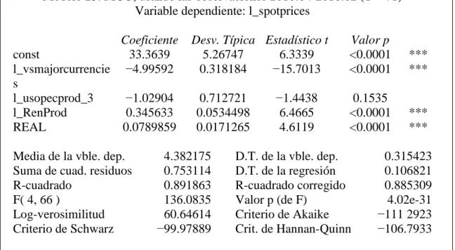
(27) Effectively, we can see how the correlations between the dependent variable and the others are negative. With [1] being a perfect direct correlation, [0] does not exist any kind of correlation and [- 1] a perfect inverse correlation. A priori, the variables that have more correlation are, in this order: dollar, production of renewable energy, combined production of OPEC and US and us real interest rate. And, as we have said, all have a negative correlation.. 7.3 Model results Table 7 Ordinary Least Square. Modelo 23: MCO, usando las observaciones 2010:04-2016:02 (T = 71) Variable dependiente: l_spotprices Coeficiente const 33.3639 l_vsmajorcurrencie −4.99592 s l_usopecprod_3 −1.02904 l_RenProd 0.345633 REAL 0.0789859 Media de la vble. dep. Suma de cuad. residuos R-cuadrado F( 4, 66 ) Log-verosimilitud Criterio de Schwarz. Desv. Típica Estadístico t 5.26747 6.3339 0.318184 −15.7013 0.712721 0.0534498 0.0171265. 4.382175 0.753114 0.891863 136.0835 60.64614 −99.97889. −1.4438 6.4665 4.6119. Valor p <0.0001 <0.0001. *** ***. 0.1535 <0.0001 <0.0001. *** ***. D.T. de la vble. dep. D.T. de la regresión R-cuadrado corregido Valor p (de F) Criterio de Akaike Crit. de Hannan-Quinn. 0.315423 0.106821 0.885309 4.02e-31 −111 2923 −106.7933. The equation that below model give us is as follows: LnPricet = 33.3639 – 4.99592LnDolart + 0.07898Realt – 1.02904LnUsOpecProdt-3 + 0.3456LnRenProdt From what we can see, it seems that fixed R-square fixed quite something (0.8853) from what we can guess that the above estimated variables have a high relationship with those observed. To see it in a more graphic way, we can create a chart in which we will compare the spot prices over time estimated variable with the observed one:. 27.

(28) Graph 8 Estimated vs observed. We will now delve into the specific variables. Taking into account above results that has yielded us estimated by ordinary least squares model, all variables are significant except for the variable l_UsOpecProd_3. However, the p - value is relatively low. We will now move on explaining all the variable results, sorted by significance, in other words, sorted by importance when it comes to explain SpotPrices dependent variable: LnDolart: clearly significant with p-value less than 0.0001. As we had planned, the relationship is negative. A 1% increase in the variable that reflects the strength of the dollar, will result in a decrease of the 4.99% in barrel prices LnRenProdt: An increase in total renewable production translates into a price increase. At the beginning, it would make no sense since the oil and renewable energies are substitute goods in some way, by which a reduction of the price of one would be also that on the other. In this case the estimates get us a 1% increase in the production of renewable energy would result in an increase of the 0.07898% spot price. LnUsOpecProdt-3: The relationship comes out negative as we had planned. A 1% increase in OPEC production translates into a decrease of 1.029% in forward prices in the next quarter. Realt: In this case the relationship between America's real interest rate and the barrel price comes out positive. Contrary to what we had planned. An increase of 1 point (since it is not logarithmic) in the real interest rate, will result in an increase of 0.079% in barrel prices.. 28.

(29) 8 FORECASTING 8.1 Forecasting independent variables In this section we will simply replace the future variables given in the previous estimation made by ordinary least squares. We are not going to make a prognosis of the variables themselves, what we are going to do is to take the data forecasted by different reliable sources. The period that we are going to compare are spot prices on June 1, 2016, with the forward from June 1, 2017 and prices estimated for June 1, 2017. Remembering the estimate that our Ordinary Least Squares Model has yielded: LnPricet = 33.3639 – 4.99592LnDolart + 0.07898Realt – 1.02904LnUsOpecProdt-3 + 0.3456LnRenProdt Then we replace independent variables for the following expected data in June 2017:. β1 Log Dólar june2017: Graph 9 Dolar Index Forecast. The data collected by Barchart indicates that dollar rate according to other currencies will be 95.862 in the month in which we want to focus for the estimation.. β2 Real june2017:. Graph 10 Nominal interest forecast. Source: http://www.tradingeconomics.com/united-states/interest-rate/forecast. 29.

(30) According to Trading Economics, U.S interest rate will increase about 0.5 per cent in the next quarter and up to 1% in 2017. This would give us a nominal interest rate 1% higher from here 12 months. However, it must take into account that we have to subtract inflation to extract the real interest rate. Average expected inflation according to Statista website for 2017 is 1.54%: Graph 11: Inflation forecast. Therefore the expected real interest rate of interest expected in June 2017 would be 0.78 + 1 - 1.54 = 0.24%. β3 Log UsOpecProd march2017:. This is by far the most difficult part to predict, due to it will be based on internal policies from United States and OPEC that we didn’t know anything. Therefore, we only can trust in what they both say about ir.. So, according to US energy information. administration (EIA) " US production – which plateaued last year – to fall to 8.6 million bpd this year from an average of 9.4 million bpd last year, or 100,000 bpd lower than its previous forecast " Therefore it is expected that US production will turn down to 8.6 million barrels per day. By OPEC side, it is rather more difficult to predict the future production quotas given the closed nature of this cartel. However, the own OPEC states that "An oversupply of oil, which has led to a steep decline in the price of the commodity in recent years, could. 30.

(31) ease soon" according to IbTimes (2016). The big question is how much will decrease OPEC production. As there is no data of any official source and as we have seen that the OPEC policy has been influenced in recent years by what has made US, we can assume that it will lower its production quotas in the same way in which US will do it. According to the EIA, United States will decrease its share of production from 9.4 million to 8.6 million, 9.30%. However, we cannot assume that OPEC will also lower its quotas by 9.30%. First, because they are not in the same situation, and second because a reduction of 9.3% of the OPEC share would be excessive taking into account the large number of barrels produced per day. Therefore we are going to assume that it will decrease its production by 2%, a share that seems reasonable. It should be noted that, indeed, that 2% is a completely arbitrary number and that it is still a subjective logic. The reason for not been able to indicate an exact fee is the lack of data due to the closed nature which we mentioned before. Therefore, assuming that the US will reduce its production 9.3% and OPEC will do so by 2%, the total production of both, would be around 3577 thousand barrels per day.. β4 Log RenProd june2017: According to EIA “expects total renewables used in the electric power sector to increase by 13.0% in 2016 and by 3.3% in 2017” therefore, following the previous case, the production of renewables would be a total of: 50,757 * 1.033 = 52,431 tWh. 31.

(32) 8.2 Forecasting dependent variable Now, we have only to replace the variables in the estimated model: LnPricet = 33,3639 – 4,99592ln(93,697) + 0,07898(0,24) – 1,02904Ln(3577)+ 0.3456Ln(52,431) The result shows that the dependent variable will be: 3,969366892. That, transformed to absolute terms give us a value of $ 52,93. Thus, there is an expected prices rise $47,64 as of June. As we can see, the estimate has not given us any unreasonable results. However, the best way to see if the model has given a good result, is comparing the estimated price with future contract in the same date, i.e. June 2017: Graph 12 Crude Oil WTI Futures prices. Source: BarChart.com. 32.

(33) In addition, we can also observe as the difference is minimal with respect to future contract price: $ 52,93 front $ 51,01, just two dollars. With these results, if we trust entirely from the estimated model, we could even get an investment strategy. In this case the strategy would be to buy future contracts from July of the coming year to $51.11 now and sell them to spot price in June for $ 52,93.. 33.

(34) 9 CONCLUSSION The model estimation seems to be satisfactory although some variables do not have the expected sign. Probably since the other variables with negative sign accumulate a big weight when it comes to explaining the dependent variable. So, that can partly ‘absorb’ the negative effect of the other variables. But, although the estimate gives a priori coherent results, it not should be forgotten that the predictions of oil prices are something that turned upside down many analysts who use more advanced techniques and yet remain unable to predict it accurately. This must be borne in mind that despite the results, to carry out this work we found a double limitation. First, the first limitation comes when modelling since the ordinary least squares estimation is rather simple for something as complex and convoluted as the price of the barrel. Second, at the time of the data collection, there were certain disagreements, although minimal, according to the sources consulted. This is basically because it is difficult to control the world oil market and even more if there are organizations such as OPEC which are so obscure when it comes to show data, inform about the strategies used, futures fees, production, etc. For this reason, this work should not be taken as a perfect model in order to make a forecast on the barrel price; it should rather be taken as a first step easily expandable and improvable due to the extensive quantity and quality of various techniques existing for this purpose. In addition, this works also let us to know the convoluted world faced by analysts of this sector and how difficult is for them to have to come up with accurate predictions.. 34.

(35) 10 REFERENCES Cheong, C.W. (2009). Modeling and Forecasting Crude Oil Markets Using ARCH-type Models. Energy Policy, Vol. 37, pp.2346–2355. Chitadze, N,. 2012. The Role of the OPEC in the International Energy Market, 1(1), pp.1-8. Frankel, J 2014. The effects of interest rate on commodity prices [e-journal], Available through: Harvard University < https://www.hks.harvard.edu/fs/jfrankel/CP.htm> [Accessed 21 May 2016]. Gilmer, A., 2016. Oil prices in 2016 will be determined by these 6 factors [e-journal], Available through: Oil price <http://oilprice.com/Energy/Energy-General/Oil-Prices-in-2016-Will-BeDetermined-By-These-6-Factors.html> [Accessed 25 April 2016]. Gilmer, B,. 2016. Why are oil prices so hard to forecast? [e-journal], Available through: Forbes < http://www.forbes.com/sites/uhenergy/2016/01/19/why-are-oil-prices-so-hard-to-forecast/ > [Accessed 19 April 2016]. Gold, R. 2015. Back to the Future? Oil Replays 1980s Bust [e-journal], Available through: Wall Street Journal <http://www.wsj.com/articles/back-to-the-future-oil-replays-1980s-bust1421196361> [Accessed 21 February 2016]. Grisse, K. 2010 What drives the oil-dollar correlation? Federal Reserve of New York pp. 1-22 Hershey, R. 1989. Worrying Anew Over Oil Imports [e-journal], Available through: New York Times < ww.nytimes.com/1989/12/30/business/worrying-anew-over-oilimports.html?pagewanted=all> [Accessed 19 February 2016]. Hutchinson, M., 1990. “Aggregate demand, uncertainly and oil prices. The 1990 oil shock in comparative perspective” Bank for international settlements, Monetary and economic department. Kaufmann, R.K. (2004). “Does OPEC Matter? An Econometric Analysis of Oil Prices.” The Energy Journal, Vol. 25, pp. 67–91.. 35.

(36) Kosakowski, P., 2015. What Determines Oil Prices? [e-journal] 94 (4), Available through: Investopedia <http://www.investopedia.com/articles/economics/08/determining-oilprices.asp> [Accessed 25 April 2016].. Mean, E., 2015. OPEC’s gigantic blunder [e-journal], Available through: Energy Matters <http://euanmearns.com/opecs-gigantic-blunder> [Accessed 25 April 2016]. Myre, G 2013. The 1973 Arab Oil Embargo: The Old Rules No Longer Apply [e-journal], Available through: NPR < http://www.npr.org/sections/parallels/2013/10/15/234771573/the1973-arab-oil-embargo-the-old-rules-no-longer-apply> [Accessed 19 March 2016]. Nixon, A., 2016. Why the world of oil is changing… [e-journal], Available through: Investor Intel < http://investorintel.com/market-analysis-intel/why-the-world-of-oil-is-changing> [Accessed 9 April 2016]. Phillips, J,. 1979. The Iranian Oil crisis [e-journal], Available through: Heritage organization <http://www.heritage.org/research/reports/1979/02/the-iranian-oil-crisis> [Accessed 9 April 2016]. Shaw, D. 2009.Crude oil price Spike: the roles of market fundamentals and speculation, 1(1), pp.1-19. Singh, J., 2015. Difference between spot market and forward market [e-journal], Available through: Economics discussion < http://www.economicsdiscussion.net/differencebetween/difference-between-spot-market-and-forward-market-foreign-exchange/615 > [Accessed 7 February 2016]. Verleger, P., 1979. The U.S. crisis of 1979, Yale University pp. 1-14 Ying Fan et al, 2011. What has driven oil prices since 2000? A structural change perspective. 33(1), pp. 1082-1094.. 36.

(37) 11 APPENDICES APPENDIX 1: WTI MONTHLY SPOT PRICES. Source: U.S Energy Information Administration. 37.

(38) APPENDIX 2: TRADE WEIGHTED U.S. DOLLAR: MAJOR CURRENCIES.. Source: Federal Reserve Bank of St Louis. 38.

(39) APPENDIX 3: US PRODUCTION RATES (thousand barrels per day). Source: U.S Energy Information Administration. 39.

(40) APPENDIX 4: US NOMINAL INTEREST RATES. Source: Monthly Monetary and Financial Statistics. 40.

(41) APPENDIX 4: USA INFLATION RATES. Source: Bureau of Labor Statistics. 41.

(42) APPENDIX 5 OPEC PRODUCTION. Source: YCHARTS – Energy Information Administration. 42.

(43) APPENDIX 6 DATA USED ON OLS ESTIMATIONS. 43.

(44) 44.

(45) 45.

(46)