A Study about the Integration of the Elliptical Orbital Motion Based on a Special One Parametric Family of Anomalies

Texto completo

(1)Hindawi Publishing Corporation Abstract and Applied Analysis Volume 2014, Article ID 162060, 11 pages http://dx.doi.org/10.1155/2014/162060. Research Article A Study about the Integration of the Elliptical Orbital Motion Based on a Special One-Parametric Family of Anomalies José Antonio López Ortí,1 Francisco José Marco Castillo,1 and María José Martínez Usó2 1. Departamento de Matemáticas, Instituto de Matemáticas y Aplicaciones de Castellón, Universidad Jaume I de Castellón, 12071 Castellón, Spain 2 Departamento de Matemática Aplicada, Universidad Politécnica de Valencia, 46022 Valencia, Spain Correspondence should be addressed to José Antonio López Ortı́; [email protected] Received 26 October 2013; Revised 27 December 2013; Accepted 6 January 2014; Published 24 February 2014 Academic Editor: Benito Chen-Charpentier Copyright © 2014 José Antonio López Ortı́ et al. This is an open access article distributed under the Creative Commons Attribution License, which permits unrestricted use, distribution, and reproduction in any medium, provided the original work is properly cited. This paper aimed to address the study of a new family of anomalies, called natural anomalies, defined as a one-parameter convex linear combination of the true and secondary anomalies, measured from the primary and the secondary focus of the ellipse, and its use in the study of analytical and numerical solutions of perturbed two-body problem. We take two approaches: first, the study of the analytical development of the basic quantities of the two-body problem to be used in the analytical theories of the planetary motion and second, the study of the minimization of the errors in the numerical integration by an appropriate choice of parameters in our family for each value of the eccentricity. The use of an appropriate value of the parameter can improve the length of the developments in the analytical theories and reduce the errors in the case of the numerical integration.. 1. Introduction One of the main problems in celestial mechanics is the study of the motion in the solar system. In this regard, it is interesting to study the planetary theories and the motion of an artificial satellite around the Earth. To construct a planetary theory, we can follow two main ways: one, the use of a numerical integrator, and two, the use of analytical methods to integrate the problem [1–4]. This paper is focused on planetary theories in the second sense. The analytical and semianalytical planetary theories involve the management of very long Poisson series developments [5] using, as temporal variables, the mean longitudes of the planets. In this sense, the study of a change of the temporal variable in order to obtain developments that are more compact than the ones obtained if the mean longitudes (or mean anomalies) are used [6–9] can be interesting. To construct an analytical or semianalytical planetary theory, it is necessary to obtain a set of developments for the twobody problem, and from that, we can evaluate the inverse of the distance between the two planets and so to develop. the second member of the differential equations of motion. Obtaining precise developments of the inverse of the distance is one of most important problems to construct the analytical theories. To study the motion of an artificial satellite, it is more convenient to use a numerical integration method. An excellent overview on numerical integrators can be seen in [10] containing a theory of symplectic and symmetric integrator, including Runge-Kutta (composition, splitting, . . .) and multistep and specially designed integrators, also their construction and practical merits are discussed. However, the history of modern numerical integrators begins long ago. Adams introduced a multistep method to study the perturbed motion of the couple Jupiter-Saturn, Kutta introduced at the beginning of the 20th century the well known family of Runge-Kutta integrators, Bulirsch and Stoer developed extrapolation methods that were used by the Institute of Applied Astronomy of St. Petersburg to obtain the minor planet ephemerides, and so forth. Numerical integrators are appropriate to study the planetary theories and the satellite motion. In the first case,.

(2) 2. Abstract and Applied Analysis. it is very important for the errors of the methods to be bounded for a very large time span and for this purpose, symplectic integrators can be adequate. One of the most important problems in the study of a satellite motion is the case of very high eccentricities. The main problem with using the mean anomaly in this case is the non uniformity on the point distribution on the ellipse due to the second Kepler law; this, for a constant step size, implies a minor concentration of points in the perigee and so larger errors in this region. In this case, it can be convenient to use a technique known as analytical regularization of step size. This technique involves a change of the temporal variable in order to have,for the new variable, a point distribution containing a major density of points in the orbital regions, where the velocity is higher. In this context, Sundman [11] introduces a new temporal variable 𝜏 related to the time 𝑡 through 𝑑𝑡 = 𝐶𝑟𝑑𝜏. Nacozy [12], Janin and Bond [13, 14], and Velez and Hilinski [15] extend this technique defining a new one-parameter family of transformations 𝛼 called generalized Sundman transformations: 𝑑𝑡 = 𝑄 (𝑟, 𝛼) 𝑑𝜏𝛼 ,. In Section 5, we obtain the differential equations of motion using an arbitrary anomaly from the natural family. A set of numerical examples about the two-body problem are analyzed. We carry out a perturbed problem in order to analyze the robustness of the method. In Section 6, the main conclusions and remarks of this paper are exposed.. 2. Basic Equations The analytical methods are based on the solution of the twobody problem (Sun planet) through a set of orbital elements, for example, the third set of Brouwer and Clemence [18] (𝑎, 𝑒, 𝑖, Ω, 𝜔, 𝑀), where 𝑀 = 𝑀0 + 𝑛(𝑡 − 𝑡0 ), 𝑛 is the mean motion, and 𝑡0 is the initial epoch being (𝑎, 𝑒, 𝑖, Ω, 𝜔, 𝑛) constants in the unperturbed two-body problem. This solution can be used as a first approximation of the perturbed problem and we can use the Lagrange method of variation of constants to replace the first elements by the osculating ones given by the Lagrange planetary equations [19]:. (1). 2 𝜕𝑅 𝑑𝑎 = , 𝑑𝑡 𝑛𝑎 𝜕𝜎. 𝛼. where 𝑄(𝑟, 𝛼) = 𝐶𝛼 𝑟 is the called partition function. A more complicated transformation was introduced by Ferrándiz et al. [16] 𝑄(𝑟) = 𝑟2/3 (𝑎0 + 𝑎1 𝑟)−1/2 and Brumberg [17] who proposed the use of the regularized length of arc: 𝑄 (𝑟) =. √𝑟 1 , √2𝐺𝑀 √1 − 𝑟/2𝑎. (2). where 𝐺𝑀 is the spaceflight constant of the Earth and 𝑎 the major semiaxe of the osculating elliptic orbit of the satellite. In this paper, we follow this technique. In particular, we propose a new one-parametric family of anomalies, called natural anomalies, defined by a convex linear combination Ψ𝛼 = 𝛼𝑓 + (1 − 𝛼)𝑓󸀠 , where 𝑓 is the true anomaly and 𝑓󸀠 the polar angle referred to the secondary focus called secondary true anomaly. The rest of this article is organized as follows. In Section 2, we introduce the general background. This section contains the equations of the perturbed motion in two ways: first, to study the analytical planetary theories and second, to use appropriate numerical methods. In Section 3, the properties of natural family of anomalies are also described. These properties include the connection between the quantities 𝑟 and 𝑟󸀠 with 𝑓󸀠 , the connection between the natural anomaly Ψ𝛼 and the eccentric anomaly 𝐸, and the study of the partition function denoted by 𝑄𝛼 (𝑟) for this case. In Section 4, the analytical developments according to the natural anomaly are studied. This study contains the developments of 𝐸, sin 𝐸, cos 𝐸, and 1/𝑟 with respect to the natural anomaly. So, an appropriate use of them is enough to obtain the development of the mean anomaly according to the natural anomaly, that is the Kepler equation. In this section, we show the length of the analytical development of the inverse of the distance for the couple Jupiter-Saturn using several values of the 𝛼.. √1 − 𝑒2 𝜕𝑅 1 − 𝑒2 𝜕𝑅 𝑑𝑒 =− + , 𝑑𝑡 𝑛𝑎2 𝑒 𝜕𝜔 𝑛𝑎2 𝑒 𝜕𝜎 ctg 𝑖 𝜕𝑅 𝜕𝑅 𝑑𝑖 1 =− + , 2 2 2 2 𝑑𝑡 𝑛𝑎 √1 − 𝑒 sin 𝑖 𝜕Ω 𝑛𝑎 √1 − 𝑒 𝜕𝜔 𝜕𝑅 𝑑Ω 1 = , 2 2 𝑑𝑡 𝑛𝑎 √1 − 𝑒 sin 𝑖 𝜕𝑖. (3). 𝜕𝑅 𝑑𝜔 √1 − 𝑒2 𝜕𝑅 cos 𝑖 = − , 2 2 2 𝑑𝑡 𝑛𝑎 𝑒 𝜕𝑒 𝑛𝑎 √1 − 𝑒 sin 𝑖 𝜕𝑖 𝑑𝜎 2 𝜕𝑅 1 − 𝑒2 𝜕𝑅 =− − , 𝑑𝑡 𝑛𝑎 𝜕𝑎 𝑛𝑎2 𝑒 𝜕𝑒 where 𝜎 is a new variable defined by the equation: 𝑡. 𝑀 = 𝜎 + ∫ 𝑛 𝑑𝑡 𝑡0. (4). and it coincides with 𝑀0 in the case of the unperturbed motion. 𝑅 is the disturbing potential 𝑅 = ∑𝑁 𝑘=1 𝑅𝑖 due to the disturbing bodies 𝑖 = 1, . . . , 𝑁. It is defined as [19] 𝑁. 𝑅 = ∑ 𝐺𝑚𝑘 [( 𝑘=1. 𝑥 ⋅ 𝑥𝑘 + 𝑦 ⋅ 𝑦𝑘 + 𝑧 ⋅ 𝑧𝑘 1 )− ], Δ𝑘 𝑟𝑘3. (5). where 𝑟 ⃗ = (𝑥, 𝑦, 𝑧) and 𝑟𝑘⃗ = (𝑥𝑘 , 𝑦𝑘 , 𝑧𝑘 ) are the heliocentric vector position of the secondary body and the 𝑘th disturbing body, respectively, Δ 𝑘 is the distance between the secondary body and the disturbing body, and 𝑚𝑘 is the mass of the disturbing body..

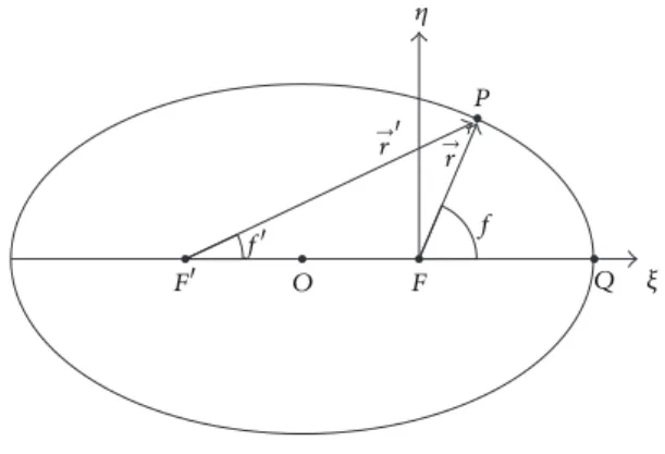
(3) Abstract and Applied Analysis. 3. In order to integrate the Lagrange planetary equations through analytical methods, it is necessary to develop the second member of the Lagrange planetary equations as truncated Fourier series, which is a classical problem in celestial mechanics [4, 5, 18, 20, 21]. The analytical methods are appropriated to study planetary motion because the eccentricities of the planetary orbits are small. Despite this, analytical methods provide very long series solution and it is convenient to obtain more compact developments using as temporal variable an appropriate anomaly [6, 7]. To obtain the developments with respect to an anomaly Ψ𝑖 , it is necessary to obtain for each planet 𝑖 the developments of the coordinates and the inverse of the radius in Fourier series of Ψ𝑖 . Then, the integration of the Lagrange planetary equations with respect to the Ψ𝑖 anomalies requires to obtain solution of the corresponding Kepler equation 𝑀𝑖 = 𝑀𝑖 (Ψ𝑖 ), for each planet. To use numerical integration methods it is more appropriate to consider the equation of motion in the form of the second Newton law. To study the efficiency of the numerical integration methods using an anomaly Ψ as temporal variable, we select the problem of the motion of an artificial satellite around the Earth. The relative motion of the secondary with respect to the Earth is defined by the second order differential equations 2. 𝑟⃗ 𝑑 𝑟⃗ ⃗ − 𝐹,⃗ = −𝐺𝑀 3 − ∇𝑈 𝑑𝑡2 𝑟. 𝜂. r. 󳰀. 3. Natural Anomalies In this section, a new family of anomalies depending on a parameter is defined. Let us represent in Figure 1 the elliptic orbit corresponding to the motion of the two-body problem. This ellipse is defined by its major semiaxis 𝑎 = 𝑂𝑄 and its eccentricity 𝑒 = 𝑐/𝑎, 0 ≤ 𝑒 < 1, where 𝑐 is the focal semidistance 𝑐 = 𝐹𝐹󸀠 /2, and the minor semiaxis 𝑏 is defined as 𝑏 = 𝑎√1 − 𝑒2 . Let 𝑂 be the center of the ellipse, let 𝐹 be the primary focus, let 𝐹󸀠 be the secondary focus (also called equality point), let 𝑄 be the pericenter, and let 𝑃 be the position of the secondary in the orbit. Let us define the coordinates (𝜉, 𝜂) referred to the primary focus and let 𝑟 and 𝑟󸀠 be the distance between the secondary 𝑃 and the primary focus and the secondary focus, 𝐹 and 𝐹󸀠 , respectively.. →. r. f. f󳰀 O. F. Q. F. 𝜉. Figure 1: Elliptic motion.. The angle 𝑓 is called the true anomaly and for the angle 𝑓󸀠 , we propose the name “secondary true anomaly”. The quantities 𝑟 and 𝑟󸀠 satisfy 𝑟 + 𝑟󸀠 = 2𝑎,. 𝑟=. 𝑎2 (1 − 𝑒2 ) 1 + 𝑒 cos 𝑓. , 𝑟󸀠 =. 𝑎2 (1 − 𝑒2 ) 1 − 𝑒 cos 𝑓󸀠. .. (7). On the other hand, the coordinates of the secondary with respect to the primary, in the orbital plane, are 𝜉 = 𝑟 sin 𝑓 = 𝑟󸀠 sin 𝑓󸀠 = 𝑎 (𝑒 − cos 𝐸) , (8). (6). where 𝑟 ⃗ is the radius vector of the satellite, 𝑈 the potential from which the perturbative conservative forces are derived, and 𝐹⃗ includes the nonconservative forces. To integrate system (6), it is necessary to know the initial values of the radius vector 𝑟0⃗ and velocity V⃗0 . In order to uniformize the truncation errors when a numerical integrator is used, there are three main ways: the use of a very small stepsize, the use of a adaptive stepsize method, and the use of a change in the temporal variable to get an appropriate distribution of the points in the orbit so that the points are mostly concentrated in the regions where the speed and curvature are maxima. In this paper, we follow the third way, as previously stated.. P. →󳰀. 𝜂 = 𝑟 cos 𝑓 = 𝑟󸀠 cos 𝑓󸀠 − 2𝑎𝑒 = 𝑎√1 − 𝑒2 sin 𝐸. The spatial orbital coordinates 𝑟 ⃗ = (𝑥, 𝑦, 𝑥)𝑡 are related to the orbital coordinates (𝜉, 𝜂, 0)𝑡 by means of ⃗ , 𝑟 ⃗ = 𝐴𝑟orb. (9). where 𝐴 = 𝑅1 (−Ω)𝑅3 (−𝑖)𝑅1 (−𝜔). 𝑅𝑖 defines a rotation around the 𝑖-axis. From (7) we have 𝑑𝑟 + 𝑑𝑟󸀠 = 0,. 𝑑𝑟 = −. 𝑎2 (1 − 𝑒2 ) sin 𝑓𝑑𝑓 2. (1 + 𝑒 cos 𝑓). , (10). 𝑑𝑓󸀠 =. 2. 2. 󸀠. 𝑎 (1 − 𝑒 ) sin 𝑓 𝑑𝑓. 󸀠. 2. (1 − 𝑒 cos 𝑓󸀠 ). and from (10), it is easy to obtain 𝑟2 sin 𝑓𝑑𝑓 = 𝑟󸀠2 sin 𝑓󸀠 𝑑𝑓󸀠 . Taking into account (8), we obtain 𝑟𝑑𝑓 = 𝑟󸀠 𝑑𝑓󸀠 .. (11). The radii 𝑟 and 𝑟󸀠 are related to the eccentric anomaly 𝐸 through 𝑟 = 𝑎 (1 − 𝑒 cos 𝐸) ,. 𝑟󸀠 = 𝑎 (1 + 𝑒 cos 𝐸) .. (12). The anomalies 𝑓 and 𝑓󸀠 are related to the eccentric anomaly 𝐸 by tan. 𝑓 1+𝑒 𝐸 =√ tan , 2 1−𝑒 2. tan. 𝑓󸀠 1−𝑒 𝐸 =√ tan . (13) 2 1+𝑒 2.

(4) 4. Abstract and Applied Analysis. To relate the anomaly 𝑓󸀠 to the mean anomaly 𝑀 we use the integral of areas 𝑑𝑓 = (𝑎2 √1 − 𝑒2 /𝑟2 )𝑑𝑀, and after replacing in (11), we get √1 − 𝑒2 𝑎2 √1 − 𝑒2 𝑑𝑀 = 𝑑𝑀. 𝑑𝑓 = 𝑟𝑟󸀠 1 − 𝑒2 cos2 𝐸 󸀠. and consequently. ∞ 2 𝑓󸀠 = 𝐸 + ∑ (−1)𝑘 𝑞𝑘 sin 𝑘𝐸. 𝑘 𝑘=1. (14). (22). To compare 𝑓󸀠 and 𝑀 up to second order in 𝑒 we have 𝑓󸀠 = 𝑀 +. 𝑒2 sin 2𝑀 + 𝑂 (𝑒3 ) 4. (15). and so, for small values of eccentricity, the anomaly 𝑓󸀠 is near 𝑀. Let us define the natural family of anomalies Ψ𝛼 as Ψ𝛼 = 𝛼𝑓 + (1 − 𝛼) 𝑓󸀠 ,. 0≤𝛼≤1. ∞. Ψ = 𝐸 + ∑ [1 + (−1 + (−1)𝑘 ) 𝑞𝑘 𝛼] 𝑘=1. 2 sin 𝑘𝐸. 𝑘. (23). (16). this family includes, for 𝛼 = 0, the secondary true anomaly 𝑓󸀠 and, for 𝛼 = 1, the true anomaly 𝑓. The anomaly Ψ𝛼 is related to the mean anomaly by 𝑑𝑀 = 𝑄𝛼 (𝑟) 𝑑Ψ𝛼 ,. Replacing (20) and (22) in (16) we obtain. (17). From this development, we can obtain up to an arbitrary order 𝑘 in the developments, with respect to Ψ, of 𝐸 and an arbitrary analytical function 𝑓(𝐸) using the Deprit inversion algorithm [23]. As an example, up to fourth order in 𝑞, we have. (18). 𝐸 = Ψ + {2 (1 − 2𝛼) 𝑞 + (8𝛼3 − 12𝛼2 + 4𝛼) 𝑞3 } sin Ψ. where the function 𝑄𝛼 (𝑟) is defined as 𝑄𝛼 (𝑟) =. 1 𝑎2 √1 − 𝑒2. 𝑟[. 𝛼 1 − 𝛼 −1 + ] . 𝑟 2𝑎 − 𝑟. + {(8𝛼2 − 8𝛼 + 1) 𝑞2. 4. Analytical Developments To integrate the planetary Lagrange equations, it is necessary to develop the second member of the Lagrange planetary equations as Fourier series with respect to the selected anomalies for each couple of planets. For this task, it is necessary to obtain for each planet the developments according to the selected anomaly of the orbital coordinates 𝜉, and 𝜂, the inverse of the radius 1/𝑟 and the mean anomaly 𝑀. For this purpose, first of all, we obtain the development of an arbitrary anomaly Ψ(𝛼) in the natural anomalies family. In the future, we will denote Ψ(𝛼) as Ψ, if it does not lead to confusion. The developments of the orbital coordinates 𝜉, 𝜂 (8) are completely determined by the ones of sin 𝐸 and cos 𝐸. To obtain these developments, it is necessary first to expand Ψ with respect to 𝐸 [22]. To relate the natural anomaly to the eccentric anomaly, it is convenient to obtain the development of the natural anomaly as Fourier series of eccentric anomaly. To this aim, it is convenient to use the classic formula [4] tan. 𝑓 1+𝑒 𝐸 1+𝑞 𝐸 =√ tan = tan , 2 1−𝑒 2 1−𝑞 2. (19). + (− × sin 2Ψ. + {−24𝛼3 + 36𝛼2 − +{. 2 𝑓 = 𝐸 + ∑ 𝑞𝑘 sin 𝑘𝐸. 𝑘 𝑘=1. (20). × sin 4Ψ (24) sin 𝐸 = {1 + (−2𝛼2 + 2𝛼 − 1) 𝑞2 +(. 4𝛼4 8𝛼3 8𝛼2 4𝛼 4 − + − ) 𝑞 } sin Ψ 3 3 3 3. + { (1 − 2𝛼) 𝑞 +(. 32𝛼3 22𝛼 − 16𝛼2 + − 1) 𝑞3 } sin 2Ψ 3 3. + {(6𝛼2 − 6𝛼 + 1) 𝑞2. The secondary true anomaly verifies 𝑓󸀠 1−𝑒 𝐸 1−𝑞 𝐸 tan =√ tan = tan 2 1+𝑒 2 1+𝑞 2. 40𝛼 2 3 + } 𝑞 sin 3Ψ 3 3. 256𝛼4 512𝛼3 320𝛼2 64𝛼 1 4 − + − + }𝑞 3 3 3 3 2. where 𝑞 = tan(𝜙/2), 𝑒 = sin 𝜙 and so ∞. 128 4 256𝛼3 160𝛼2 32𝛼 4 𝛼 + − + )𝑞 } 3 3 3 3. + (−54𝛼4 + 108𝛼3 − 72𝛼2 + 18𝛼 − 1) 𝑞4 } (21). × sin 3Ψ.

(5) Abstract and Applied Analysis + {− +{. 5. 38𝛼 64 3 𝛼 + 32𝛼2 − + 1} 𝑞3 sin 4Ψ 3 3. To develop 𝑎/𝑟 with respect to Ψ, it is more convenient to use (7) and then we have. 250𝛼4 500𝛼3 320𝛼2 70𝛼 − + − + 1} 𝑞4 3 3 3 3. 𝑎 1 + 𝑒 cos 𝑓 . = 𝑟 1 − 𝑒2 It is easy to see from (19) and (21) that. × sin 5Ψ (25) cos 𝐸 = (1 − 2𝛼) 𝑞. tan. (30). and so 2. + {1 + (−1 + 6𝛼 − 6𝛼 ) 𝑞 +(. ∞ 2 𝑓󸀠 = 𝑓 + ∑ (−1)𝑘 𝑒𝑘 sin 𝑘𝑓. 𝑘 𝑘=1. 2. 20𝛼4 40𝛼3 28𝛼2 8 4 − + − ) 𝑞 } cos Ψ 3 3 3 3. × cos 2Ψ + {(1 − 6𝛼 + 6𝛼2 ) 𝑞 + (−90𝛼4 + 180𝛼3 − 116𝛼2 + 26𝛼 − 1) 𝑞4 } × cos 3Ψ 64 38𝛼 + {− 𝛼3 + 32𝛼2 − + 1} 𝑞3 cos (4Ψ) 3 3 250𝛼4 500𝛼3 320𝛼2 70𝛼 +{ − + − + 1} 𝑞4 3 3 3 3. ∞ 2 Ψ = 𝑓 + ∑ (−1)𝑘 (1 − 𝛼) 𝑞𝑘 sin 𝑘𝑓. 𝑘 𝑘=1. cos 𝑓 = (𝛼 − 1) 𝑒 5𝛼 3𝛼2 − + 1) 𝑒2 2 2. +(. 5𝛼4 7𝛼3 13𝛼2 𝛼 4 − + − ) 𝑒 } cos Ψ 12 6 12 3. + {(1 − 𝛼) 𝑒 + ( (26). The mean anomaly 𝑀 is related to the eccentric anomaly through the Kepler equation 𝑀 = 𝐸 − 𝑒 sin 𝐸. Replacing (24) and (25) in the Kepler equation we obtain 𝑀 = Ψ + {−4𝛼𝑞 + (8𝛼3 − 8𝛼2 + 4) 𝑞3 } sin Ψ + { (8𝛼 − 4𝛼 − 1) 𝑞 2. 64𝛼 128 4 𝛼 + 64𝛼3 − 8𝛼 + 4) 𝑞4 } sin 2Ψ 3 3 4𝛼 4 3 − } 𝑞 sin 3Ψ 3 3. 256𝛼4 128𝛼2 3 +{ − 128𝛼3 + + 4𝛼 − } 𝑞4 sin 4Ψ. 3 3 2 (27) This is the Kepler equation for the natural anomaly Ψ and it is necessary to integrate the second member of planetary equation of Lagrange [8, 24]. The parameter 𝑞 is related to 𝑒 by 𝑞 = (1 − √1 − 𝑒2 )/𝑒 an so, 𝑞 can be developed as ∞. (2𝑘 − 1)!! 2𝑘−1 , 𝑒 2𝑘 𝑘! 𝑘=1. 𝑞=∑. the value of 𝑞 verifies 0 ≤ 𝑞 = 𝑒/(1 + √1 − 𝑒2 ) ≤ 𝑒.. + {(. 13𝛼 8𝛼3 − 6𝛼2 + − 1) 𝑒3 } cos 2Ψ 3 3. 3𝛼2 5𝛼 − +) 𝑒2 2 2 + (−. 45 4 63𝛼3 127𝛼2 27𝛼 𝛼 + − + − 1) 𝑒4 } 8 4 8 4. × cos 3Ψ. 2. + {−24𝛼3 + 24𝛼2 −. (32). Applying Deprit algorithm [23], we obtain the development of cos 𝑓 up to an arbitrary order in 𝑒. As an example, up to fourth order in 𝑒, we have. + {1 + (. × cos (5Ψ) .. (31). Consequently,. 38𝛼 64𝛼3 + {𝑞 + ( − 32𝛼2 + − 2𝛼𝑞 − 1) 𝑞3 } 3 3. + (−. 𝑓󸀠 1 − 𝑒 𝑓 = tan 2 1+𝑒 2. (29). (28). 13𝛼 8 + 1} 𝑒3 cos 4Ψ + {− 𝛼3 + 6𝛼2 − 3 3 +{. 125𝛼4 175𝛼3 355𝛼2 77𝛼 − + − + 1} 𝑒4 cos 5Ψ. 24 12 24 12 (33). Replacing (33) in (29) finally we obtain 𝑎 = 1 + 𝛼𝑒4 + 𝛼𝑒2 𝑟 3 5𝛼 3 + {𝑒 + (− 𝛼2 + ) 𝑒 } cos Ψ 2 2 + {(1 − 𝛼) 𝑒2 + ( +{. 8𝛼3 10𝛼 4 − 6𝛼2 + ) 𝑒 } cos 2Ψ 3 3. 3𝛼2 5𝛼 − + 1} 𝑒3 cos 3Ψ 2 2. 13𝛼 8 + {− 𝛼3 + 6𝛼2 − + 1} 𝑒4 cos 4Ψ. 3 3 (34).

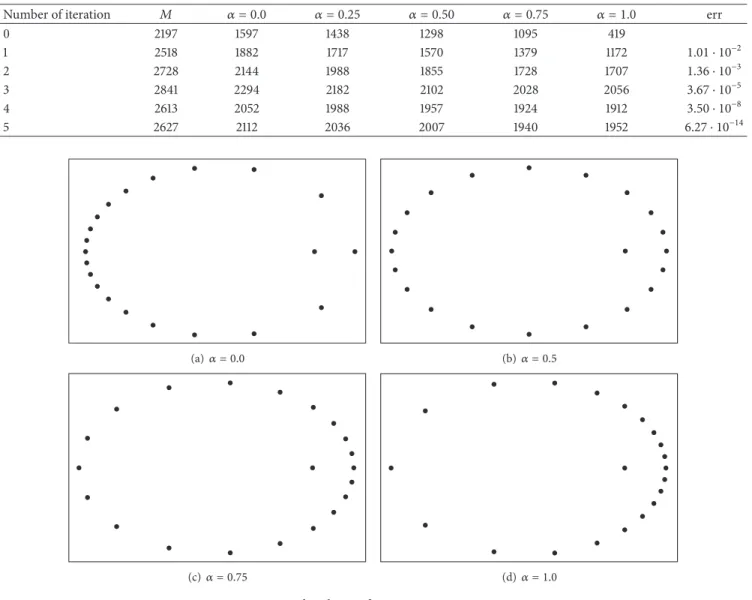
(6) 6. Abstract and Applied Analysis Table 1: Length of the 1/Δ using 𝑀, Ψ0 , Ψ0.25 , Ψ0.5 , Ψ0.75 , and Ψ1.0 .. Number of iteration 0 1 2 3 4 5. 𝑀 2197 2518 2728 2841 2613 2627. 𝛼 = 0.0 1597 1882 2144 2294 2052 2112. 𝛼 = 0.25 1438 1717 1988 2182 1988 2036. 𝛼 = 0.50 1298 1570 1855 2102 1957 2007. 𝛼 = 0.75 1095 1379 1728 2028 1924 1940. (a) 𝛼 = 0.0. (b) 𝛼 = 0.5. (c) 𝛼 = 0.75. (d) 𝛼 = 1.0. 𝛼 = 1.0 419 1172 1707 2056 1912 1952. err 1.01 ⋅ 10−2 1.36 ⋅ 10−3 3.67 ⋅ 10−5 3.50 ⋅ 10−8 6.27 ⋅ 10−14. Figure 2: Points distribution for 𝑒 = 0.7, 𝛼 = 0.0, 0.5, 0.75, 1.0.. 0.95 0.90 0.85 0.80 0.75 0.2. 0.4. 0.6. 0.8. Figure 3: Optimal value of 𝛼 for each value of 𝑒 ∈ [0, 0.95].. The convergence of these developments is poor when the eccentricity is near to one. Fortunately, in the case of the planetary motion, the eccentricity values are small and the convergence rate is appropriate. On the other hand, for. intermediate values of eccentricity, the length of the series using an appropriate anomaly Ψ𝛼 is lower than if the mean anomaly is used as temporal variable. The main problem to develop the second member of the Lagrange planetary equations is to develop the inverse of the distance. This development can be obtained using the Kovalevsky algorithm [25]. Table 1 shows, for the couple Jupiter-Saturn, the performance of the algorithm. This table contains the length of the expansion of the inverse of the distance using the mean anomaly 𝑀 and the natural anomaly for 𝛼 = 0, 0.25, 0.50, 0.75, 1.0, and the estimated error in astronomical units for each iteration. The planetary elements are taken from [26].. 5. Numerical Examples In general, the perturbative forces are small, for this reason, it is convenient to test the methods by applying them to the well known two-body problem, referred to the orbital.

(7) Abstract and Applied Analysis. 7 ×10−4. ×10−6 6.0. 200. 4.0. 400. 600. 800. 1000. 600. 800. 1000. 600. 800. 1000. 600. 800. 1000. −0.05. 2.0 200. 400. 600. 800. 1000. −2.0. −0.1 −0.15. −4.0 −6.0. −0.2. (a) erx. (b) ery. ×10−9. −0.5. ×10 2.0 200. 400. 600. 800. −9. 1000 1.0. −1.0 −1.5. 200. −2.0. 400. −1.0. −2.5 −3.0. −2.0 (c) ervx. (d) ervy. Figure 4: Local integration errors distribution 𝑒 = 0.7, 𝛼 = 0.0. ×10−7 0.5. ×10−7 2.0. 200. 1.0 200. 400. 600. 800. 1000. 400. −0.5. −1.0 −1.0 −2.0 (a) erx. (b) ery. ×10−12. ×10. −12. 4.0 5.0. 2.0 200. 400. 600. 800. 1000 200. −2.0. 400. −4.0. −5.0. −6.0. (c) ervx. (d) ervy. Figure 5: Local integration errors distribution 𝑒 = 0.7, 𝛼 = 0.5..

(8) 8. Abstract and Applied Analysis ×10−7 1.5. ×10−7 2.0. 1.0. 1.0. 200. 400. 600. 800. 1000. 0.5. −1.0 200. 400. 600. 800. 1000. −2.0 (a) erx. ×10 1.5. (b) ery. −12. ×10−12. 1.0. 1.5. 0.5. 1.0 200. −0.5. 400. 600. 800. 1000. 0.5 200. −0.5. −1.0. 400. 600. 800. 1000. −1.0. −1.5. −1.5. −2.0. (c) ervx. (d) ervy. Figure 6: Local integration errors distribution 𝑒 = 0.7, 𝛼 = 0.75. ×10−7 3.0. ×10−7 1.5. 2.5. 1.0. 2.0. 0.5. 1.5 200. 400. 600. 800. 1000. −0.5. 1.0 0.5. −1.0 −1.5. 200 (a) erx. ×10 2.5. 400. 600. 800. 1000. (b) ery. −12. ×10. −12. 3.0. 2.0. 2.0. 1.5. 1.0. 1.0. 200. 400. −1.0. 0.5 200. 400. −0.5 (c) ervx. 600. 800. 1000. −2.0 −3.0 (d) ervy. Figure 7: Distribution of the local integration errors 𝑒 = 0.7, 𝛼 = 1.0.. 600. 800. 1000.

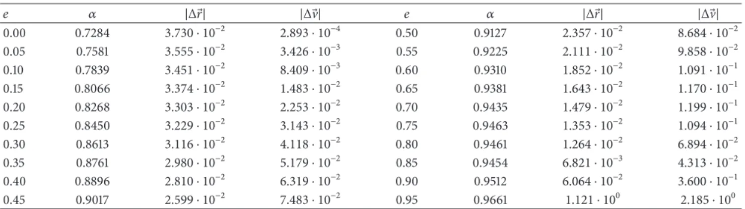
(9) Abstract and Applied Analysis. 9. coordinate system (𝑥, 𝑦, 0), to select an appropriate new temporal variable in order to minimize the distribution of the truncation errors in the orbit. Let us define a generic family Ψ𝛼 of anomalies depending on a parameter 𝛼 as 𝑑𝑡 = 𝑄𝛼 (𝑟)𝑑Ψ𝛼 . For each 𝛼 we have 𝑑 𝑑 𝑑 𝑑 𝑑Ψ𝛼 𝑛 . =𝑛 =𝑛 = 𝑑𝑡 𝑑𝑀 𝑑Ψ𝛼 𝑑𝑀 𝑄𝛼 (𝑟) 𝑑Ψ𝛼. problem, this problem includes the Earth, the Moon, and an artificial satellite with the same semiaxe that Heos II and eccentricity 0.95. The problem uses the following approach to the motion of the satellite perturbed by the Moon. (1) The satellite is in the orbital plane of the Moon.. (35). (2) The Moon motion is approached through a circular motion around the Earth with a sidereal period of 27 days 4 h 43 m 11.5 s, orbital radius of the Moon 𝑅𝐿 = 384.400 Km, and mass 0, 01231 in units of Earth mass.. 𝑄 (𝑟) 𝑑𝑥 = 𝛼 V𝑥 , 𝑑Ψ𝛼 𝑛. 𝑑V𝑥 𝑄 (𝑟) 𝑥 𝜕𝑉 =− 𝛼 [𝐺𝑀 3 + − 𝐹𝑥 ] , 𝑑Ψ𝛼 𝑛 𝑟 𝜕𝑥. (3) The couple Earth-Moon is not perturbed by the satellite motion.. 𝑑𝑦 𝑄 (𝑟) = 𝛼 V𝑦 , 𝑑Ψ𝛼 𝑛. 𝑑V𝑦. So,. 𝑑Ψ𝛼. =−. 𝑦 𝜕𝑉 𝑄𝛼 (𝑟) [𝐺𝑀 3 + − 𝐹𝑦 ] . 𝑛 𝑟 𝜕𝑦 (36). In order to test the performance of this method, we use a fictitious artificial satellite with the same elements than HEOS II used by Brumberg [17] (𝑎 = 118363.47 Km, 𝑒 = 0.942572319, 𝑖 = 28o .16096, Ω = 185o .07554, 𝜔 = 270o .07151, 𝑀0 = 0o ), except for its eccentricity, that it is changed to study the optimum value of 𝛼 depending on the value of the eccentricity 𝑒. In Figure 2, we show a sample of twenty points for Ψ𝛼 with homogeneous distribution over the orbit. Table 2 shows the values of the different 𝛼, where the minimum of the errors for this fictitious satellite with the same (𝑎, 𝑖, Ω, 𝜔, 𝑀) elements than HEOSII and different values of eccentricity (𝑒 = 0.0, 0.05, . . . , 0.95) is reached. This table has been carried out using a classic Runge Kutta integrator of fourth order with 1000 uniform steps. In this table, we can see that the value of 𝛼, where the errors in position reach their minimum, depends on the eccentricity. A least square analytical approach to the optimal value of 𝛼 can be written as 𝛼 = 2.10826𝑒5 − 4.77809𝑒4 + 3.92513𝑒3 −1.71554𝑒2 + 0.71606𝑒 + 0.72724 .. (37). Figure 3 shows the value of 𝛼, where the error |Δ𝑟|⃗ reaches its minimum for each value of 𝑒 ∈ [0, 0.95] and its analytical approximation. Figures 4, 5, 6 and 7 show the local integration errors, in position and velocity, for a satellite with 𝑎 = 118363.47 Km and 𝑒 = 0.7 for the values of 𝛼 = 0, 0.5, 0.75, 1.0. These errors have been obtained solving for each value of Ψ𝛼 the equation Ψ𝛼 = Ψ𝛼 (𝐸). From the value of 𝐸, we compute, using the two-body equations, the exact solution for the position and velocity vectors. These values are the initial conditions for the numerical integrator. The local truncation errors are exactly evaluated by comparing the values obtained through integration in the next step with the corresponding ones evaluated solving the equation Ψ𝛼 + ℎ = Ψ𝛼 (𝐸). The solution of the equation Ψ𝛼 = Ψ𝛼 (𝐸) is obtained solving, for each value of Ψ𝛼 = 𝑖 ∗ ℎ, (16) and (13). To test the robustness of the method, we will study a perturbed case included in the planar restricted three-body. Table 3 shows the number of steps necessary to provide an accuracy of 10−4 Km in position in an integration over 100 days using as integrator a classic Runge-Kutta of fourth order and a Runge-Kutta of order eight [27]. To evaluate the global error, we have compared the position results using 𝑁 and 1.1 𝑁 steps. In this table, we can see that the integration can be improved by the use of an appropriate choice of 𝛼 in the natural family of anomalies given by 𝛼(𝑒) (37). It is important to emphasize that all the anomalies of this family improve the values obtained by the use of the mean anomaly.. 6. Concluding Remarks In this paper, a new one-parametric family of anomalies, called natural anomalies, has been defined. This family of anomalies is adequate to be used in the construction of the analytical theories of planetary motion. In this sense, we have described a method to obtain the analytical development as Fourier series of the natural anomaly up an arbitrary order in eccentricity of the most common quantities (25), (26), and (29) of the two-body problem, and from these developments, we can obtain the development of the second member of the Lagrange planetary equation. To test the efficiency of the use of the variables Ψ𝛼 as independent variables in the analytical developments, we show the performance of the Kovalevsky algorithm to obtain the inverse of the distance for the couple Jupiter-Saturn, obtaining more compact developments for values of 𝛼 near to values given by (37). To integrate the Lagrange planetary equations by analytical methods using a generalized anomaly as temporal variable, it is necessary to use the generalized Kepler equation (27). The natural anomalies conform to a parametric family of anomalies that includes the true anomaly. For 𝛼 = 0, we have the secondary true anomaly, its value being near to the mean anomaly for small values of the eccentricity and, in the case of an eccentricity that is not small, the spatial points distribution over the orbit is the most appropriate, if the mean anomaly is used. In the symmetrical case, Ψ1/2 defines a point distribution over the orbit with a major concentration in the perigee than if the eccentric anomaly 𝐸 is used. The two-body problem has been used to test the performance of the numerical integrators. In this study, the local and global errors depend on the value of 𝛼. The global.

(10) 10. Abstract and Applied Analysis Table 2: Optimal 𝛼 for 𝑒|Δ𝑟|⃗ in 10−5 Km |ΔV|⃗ in 10−8 Km/s.. 𝑒 0.00 0.05 0.10 0.15 0.20 0.25 0.30 0.35 0.40 0.45. 𝛼 0.7284 0.7581 0.7839 0.8066 0.8268 0.8450 0.8613 0.8761 0.8896 0.9017. |Δ𝑟|⃗ 3.730 ⋅ 10−2 3.555 ⋅ 10−2 3.451 ⋅ 10−2 3.374 ⋅ 10−2 3.303 ⋅ 10−2 3.229 ⋅ 10−2 3.116 ⋅ 10−2 2.980 ⋅ 10−2 2.810 ⋅ 10−2 2.599 ⋅ 10−2. |ΔV|⃗ 2.893 ⋅ 10−4 3.426 ⋅ 10−3 8.409 ⋅ 10−3 1.483 ⋅ 10−2 2.253 ⋅ 10−2 3.143 ⋅ 10−2 4.118 ⋅ 10−2 5.179 ⋅ 10−2 6.319 ⋅ 10−2 7.483 ⋅ 10−2. Table 3: Number of steps to get a precision of |Δ𝑟|⃗ < 10−4 Km. 𝑁 𝛼 = 0 𝛼 = 0.25 𝛼 = 0.5 𝛼 = 0.75 𝛼 = 1.0 𝛼(𝑒) RK4 7084079 3292627 401504 251229 190193 158367 146393 RK8 305033 94362 14303 10833 9025 6840 6630. integration errors in a revolution depend on 𝛼. This value increases with the eccentricity, and it is near 0.72 for lower eccentricities and 0.9661 for higher ones (𝑒 = 0.95). To test the robustness of the method, a simplified problem, included in the restricted three-body problem, has been analyzed. In this problem, we study the number of steps that is necessary to get a precision of 1 ⋅ 10−4 Km in |Δ𝑟|⃗ using a classical method of Runge-Kutta of fourth order and a RungeKutta of eighth order. The number of steps is minimum when we take for each step the value of 𝛼 that minimizes the error in the osculating two-body problem (37). The result is similar using a classic RK4 method and using a RK8 method, obviously with a minor number of steps in the last case.. Conflict of Interests The authors declare that there is no conflict of interests regarding the publication of this paper.. Acknowledgment This research has been partially supported by Grant P1.1B2012-47 from University Jaume I of Castellón.. References [1] P. Bretagnon and G. Francou, “Variations seculaires des orbites planetaires. Théorie VSOP87,” Astronomy & Astrophysics, vol. 114, pp. 69–75, 1988. [2] J. L. Simon, “Computation of the first and second derivatives of the Lagrange equations by harmonic analysis,” Astronomy & Astrophysics, vol. 17, pp. 661–692, 1982. [3] J. L. Simon, G. Francou, A. Fienga, and H. Manche, “New analytical planetary theories VSOP2013 and TOP2013,” Astronomy & Astrophysics, vol. 557, article A49, 2013.. 𝑒 0.50 0.55 0.60 0.65 0.70 0.75 0.80 0.85 0.90 0.95. 𝛼 0.9127 0.9225 0.9310 0.9381 0.9435 0.9463 0.9461 0.9454 0.9512 0.9661. |Δ𝑟|⃗ 2.357 ⋅ 10−2 2.111 ⋅ 10−2 1.852 ⋅ 10−2 1.643 ⋅ 10−2 1.479 ⋅ 10−2 1.353 ⋅ 10−2 1.264 ⋅ 10−2 6.821 ⋅ 10−3 6.064 ⋅ 10−2 1.121 ⋅ 100. |ΔV|⃗ 8.684 ⋅ 10−2 9.858 ⋅ 10−2 1.091 ⋅ 10−1 1.170 ⋅ 10−1 1.199 ⋅ 10−1 1.094 ⋅ 10−1 6.894 ⋅ 10−2 4.313 ⋅ 10−2 3.600 ⋅ 10−1 2.185 ⋅ 100. [4] F. F. Tisserand, Traité de Mecanique Celeste, Gauthier-Villars, Paris, France, 1986. [5] V. A. Brumberg, Analytical Techniques of Celestial Mechanics, Springer, Berlin, Germany, 1995. [6] P. Nacozy, “Hansen’s method of partial anomalies: an application,” The Astronomical Journal, vol. 74, pp. 544–550, 1969. [7] E. Brumberg and T. Fukushima, “Expansions of elliptic motion based on elliptic function theory,” Celestial Mechanics and Dynamical Astronomy, vol. 60, no. 1, pp. 69–89, 1994. [8] J. A. López and M. Barreda, “A formulation to obtain semianalytical planetary theories using true anomalies as temporal variables,” Journal of Computational and Applied Mathematics, vol. 204, no. 1, pp. 77–83, 2007. [9] J. A. López Ortı́, M. J. Martı́nez Usó, and F. J. Marco Castillo, “Semi-analytical integration algorithms based on the use of several kinds of anomalies as temporal variable,” Planetary and Space Science, vol. 56, no. 14, pp. 1862–1868, 2008. [10] E. Hairer, C. Lubich, and G. Wanner, Geometric Numerical Integration, Springer, Heidelberg, Germany, 2006. [11] K. Sundman, “Memoire sur le probleme des trois corps,” Acta Mathematica, vol. 36, no. 1, pp. 105–179, 1913. [12] P. Nacozy, “The intermediate anomaly,” Celestial Mechanics, vol. 16, no. 3, pp. 309–313, 1977. [13] G. Janin, “Accurate computation of highly eccentric satellite orbits,” Celestial Mechanics, vol. 10, no. 4, pp. 451–467, 1974. [14] G. Janin and V. R. Bond, “The elliptic anomaly,” NASA Technical Memorandum 58228, 1980. [15] C. E. Velez and S. Hilinski, “Time transformations and cowell’s method,” Celestial Mechanics, vol. 17, no. 1, pp. 83–99, 1978. [16] J. M. Ferrándiz, S. Ferrer, and M. L. Sein-Echaluce, “Generalized elliptic anomalies,” Celestial Mechanics, vol. 40, no. 3-4, pp. 315– 328, 1987. [17] E. V. Brumberg, “Length of arc as independent argument for highly eccentric orbits,” Celestial Mechanics and Dynamical Astronomy, vol. 53, no. 4, pp. 323–328, 1992. [18] D. Brouwer and G. M. Clemence, Celestial Mechanics, Academic Press, New York, NY, USA, 1965. [19] J. J. Levallois and J. Kovalevsky, Géodésie Générale, vol. 4, Eyrolles, Paris, France, 1971. [20] Y. Hagihara, Celestial Mechanics, MIT Press, Cambridge, Mass, USA, 1970. [21] J. Kovalewsky, Introduction to Celestial Mechanics, D. Reidel, Dodrecht, The Netherlands, 1967..

(11) Abstract and Applied Analysis [22] J. A. López, V. Agost, and M. Barreda, “A note on the use of the generalized sundman transformations as temporal variables in celestial mechanics,” International Journal of Computer Mathematics, vol. 89, pp. 433–442, 2012. [23] A. Deprit, “Note on Lagrange’s inversion formula,” Celestial Mechanics, vol. 20, no. 4, pp. 325–327, 1979. [24] J. A. López, M. Barreda, and J. Artes, “Integration algorithms to construct semi-analytical planetary theories,” Wseas Transactions on Mathematics, vol. 5, no. 6, pp. 609–614, 2006. [25] J. Chapront, P. Bretagnon, and M. Mehl, “Un formulaire pour le calcul des perturbations d’ordres élevés dans les problèmes planétaires,” Celestial Mechanics, vol. 11, no. 3, pp. 379–399, 1975. [26] J. L. Simon, P. Bretagnon, P. Chapront, J. Chapront-Touzé, G. Francou, and J. Laskar, “Numerical expressions for precession formulae and mean elements for the Moon and the planets,” Astronomy & Astrophysics, vol. 282, pp. 663–683, 1994. [27] E. Fehlberg and G. C. Marsall, “Classical fifth, sixth, seventh and eighth runge-kutta formulas with stepsize control,” NASA Technical Report R-287, 1968.. 11.

(12) Advances in. Operations Research Hindawi Publishing Corporation http://www.hindawi.com. Volume 2014. Advances in. Decision Sciences Hindawi Publishing Corporation http://www.hindawi.com. Volume 2014. Journal of. Applied Mathematics. Algebra. Hindawi Publishing Corporation http://www.hindawi.com. Hindawi Publishing Corporation http://www.hindawi.com. Volume 2014. Journal of. Probability and Statistics Volume 2014. The Scientific World Journal Hindawi Publishing Corporation http://www.hindawi.com. Hindawi Publishing Corporation http://www.hindawi.com. Volume 2014. International Journal of. Differential Equations Hindawi Publishing Corporation http://www.hindawi.com. Volume 2014. Volume 2014. Submit your manuscripts at http://www.hindawi.com International Journal of. Advances in. Combinatorics Hindawi Publishing Corporation http://www.hindawi.com. Mathematical Physics Hindawi Publishing Corporation http://www.hindawi.com. Volume 2014. Journal of. Complex Analysis Hindawi Publishing Corporation http://www.hindawi.com. Volume 2014. International Journal of Mathematics and Mathematical Sciences. Mathematical Problems in Engineering. Journal of. Mathematics Hindawi Publishing Corporation http://www.hindawi.com. Volume 2014. Hindawi Publishing Corporation http://www.hindawi.com. Volume 2014. Volume 2014. Hindawi Publishing Corporation http://www.hindawi.com. Volume 2014. Discrete Mathematics. Journal of. Volume 2014. Hindawi Publishing Corporation http://www.hindawi.com. Discrete Dynamics in Nature and Society. Journal of. Function Spaces Hindawi Publishing Corporation http://www.hindawi.com. Abstract and Applied Analysis. Volume 2014. Hindawi Publishing Corporation http://www.hindawi.com. Volume 2014. Hindawi Publishing Corporation http://www.hindawi.com. Volume 2014. International Journal of. Journal of. Stochastic Analysis. Optimization. Hindawi Publishing Corporation http://www.hindawi.com. Hindawi Publishing Corporation http://www.hindawi.com. Volume 2014. Volume 2014.

(13)