TítuloFundamentals and Applications of DEA

Texto completo

(1)Fundamentals and Applications of DEA C.A. Gracia-Fernández, S. Gómez-Barreiro, Lisardo Núñez-Regueira Research Group TERBIPROMAT, Departamento Física Aplicada, Universidade de Santiago de Compostela. Av. J. M. Suárez Núñez, 15782 Santiago, Spain [email protected] 1. Introduction Dielectric techniques have been used to follow chemical reactions since many years ago. In 1934, Kienle and Race reported a study on poliesterification reactions using dielectric measurements. In this forward paper, many of the important issues in nowadays studies were identified. Among these issues were included: the correlation between conductivity and viscosity, the fact that conductivity does not present sudden changes at gelation, the fact that ionic conductivity generally governs the observed dielectric properties, etc. A constant in all branches of science is that the study starts by the simplest system, thus needing only few parameters to go on. As the complexity of the system increases, more parameters are needed and a series of approaches, that reduce the grade of veracity of the equation, must be introduced. This is the case of both dielectric analysis and polymer studies. The application of dielectric analysis technique to simple molecules is certainly easy. However, the polymers are systems with such a complexity that there is no model who explains their behaviour in the two most relevant variables: temperature and frequency. In fact, the glassy transition, one of most decisive characteristics in the properties of a polymer, is not completely understood from the theoretical point of view. This is the reason why the mathematical expressions that relate the different variables involved in the system are often experimental. Some of these equations are those developed by Arrhenius, Vogel, Williams-Landel-Ferry, Cole-Cole, Cole-Davison and Havriliak-Negami, each of them valid for different conditions and states of aggregation of different classes of polymers. From 1958, many articles were reported mainly on epoxy materials. Some of the problems that disturbed this field have been the excessive empirical nature of the research, hampered by the use of the deficient models measurements have been connected in very few cases with measurements of other properties of interest. 2. Dielectric Analysis (DEA) Dielectric analysis measures changes in the properties of a material as it is submitted to a cyclic (commonly) electric field. It can supply information on: Dielectric properties thermal transition, molecular relaxation, rate of cure, degree of cure, etc. DEA follow the complete transformation of a thermoset from a low-molecularweight compound to a solid crosslinked system of infinite molecular weight. The use of disposable microdielectric sensors allows dielectric measurements to be made in the laboratory as well as into reactive manufacturing processes. The information on dielectric properties can be obtained almost instantaneously without significant.

(2) 226. LISARDO NÚÑEZ, CARLOS GRACIA-FERNÁNDEZ, SILVIA GÓMEZ-BARREIRO. disturbance of the process. Electrical properties of polymer, such as: permittivity, loss factor and conductivity can be directly obtained by dielectric analysis. To perform dielectric measurements, the material is situated in the middle of two electrodes, and a periodic voltage is applied between the electrodes. This voltage originates an electric field in the sample. In response to this electric field, displacement of charged units takes place in the material giving rise to polarization and ionic conduction; that is, to a current whose amplitude is dependent on the frequency the measurement and, also, on the temperature and structural properties of the material under studies. 3. Basic principles As it was previously mentioned, dielectric analysis is related to the measurement and characterisation of the reaction of a material to an applied periodic electric field. For this study, the material is situated between two electrodes, a sinusoidal voltage is applied across the electrodes and the current response is measured. On a molecular point of view, the current consists of a displacement of electrical charged units in the sample material. The charged units can be dipoles or mobile units (free electrons, ions). In the case of dipoles, they will align in the direction of the applied field. If the charged units are mobile, the electric field will originate conduction of net charge from one electrode to the other. In the case of polymers, both dipoles and mobile charges are present. The applied electric field gives rise to polarization and ionic conduction. The sum of polarization plus conduction is the current to be measured. This current is at the same frequency as the voltage, but is shifted in phase and amplitude. Both the phase angle and the relative amplitude change are related to the properties of the sample between the electrodes. To interpret frequency and phase difference in terms of the dielectric properties of the material it is necessary to have data on the electrode. The electrodes assembly plays a twofold role. On the hand it transmits the applied voltage to the sample, on the other hand, it collects the response current. The applied electric field E, is related to the current density, J through the relative complex dielectric constant of the sample, ε* J=iwε* E. (1). where i is the imaginary unit = √-1, ωis the angular frequency (rad s-1) and ε0 is the permittivity of free space (8,85x10-12 F m-1). It is assumed that the medium is homogeneous and its behaviour is linear respect to the electric field. The complex dielectric constant is defines as:. ε * = ε ´−iε ´´. (2). where ε´ is the relative bulk permittivity and ε´´ is the relative bulk loss factor, both are frequency dependent and depends also on temperature and the structure of the material sample. The ratio ε´´/ε´ is known as the loss tangent or dissipation, tan δ. Both the permittivity and the loss factor are the characteristic dielectric properties of a material..

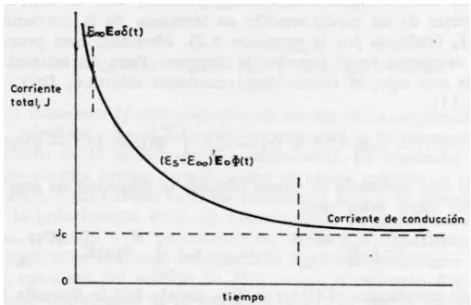
(3) FUNDAMENTALS AND APPLICATIONS OF DEA. 227. The relative permittivity, ε´, is related to the capacitive or energy storing ability of a material, and measures the electrical polarization of the sample per unit applied electric field. It is composed of the unrelaxed permittivity εu, that some investigators expressed as ε∞, the baseline permittivity, and an additional term εd´ associated with dipole alignment: ε´ = ε∞ + εd´ (3) The unrelaxed permittivity is originated by electronic and atomic polarizations and, at low frequencies, is frequency independent. Typical dielectric studies are carried out at frequencies below 1 MHz. At frequencies of this order, and temperatures below the glass transition, there can be dipolar contributions to ε´ from restricted motions of polar groups. As the temperature decreases to low temperatures, or the frequency increases to high values, the polar groups lose the ability to orient with the applied electric field and ε´ significant decreases originating the lower transitions (β, γ, ...). The relative loss factor, ε´´, measures the energy necessary for molecular motion in a electric field. It originates from two sources: the energy losses owing to the molecular dipoles orientation εd´´, and the energy losses due to the conduction of ionic species εc´´: (4) ε´´ = εd´´ + εc´´ At temperatures well below Tg, polymers generally have loss factors less than 0.1. However when the temperature reaches the Tg value and above, the loss factor can be as high as 109. 4. Kind of experiments Thermal analysis experiments have in common that the temperature is always under complete control of the investigator. In this sense, the different experiments can be divided into two main groups: isothermal experiments, in which the temperature remains constant throughout the experiment, and dynamical experiments, where the temperature is changed (increasing or decreasing) at a fixed constant rate. Sometimes, a combination of both methods is advisable. The choice of a particular method depends on the type of study to be done. In particular, isothermal experiments are carried out when the objective is to analyse the behaviour of dielectric properties as a function of time or frequency. One other point to consider is the type of process experienced by the sample; for example, is the sample suffering a polymerization process while the experiment is taking place or, on contrary, if the sample is yet polymerized. In dynamical experiments the sample is submitted to a controlled constant heating (or cooling) rate. One of the most direct applications of this method is the study of the possible transitions of a polymerized material and, in particular, the obtention of the glass transition temperature. 4.1.. Frequency domain. One other variable that can be controlled in a dielectric analysis experiment is how the electric field can be applied either in sinusoidal or step-like form. Figure 1 shows the electric current in a dielectric polymer as a function of time when the sample is subjected to a constant electric field[1]..

(4) 228. LISARDO NÚÑEZ, CARLOS GRACIA-FERNÁNDEZ, SILVIA GÓMEZ-BARREIRO. Figure 1. Typical change of a transient current in a dielectric material. The main interest of the experiment in which the electric field is step.like applied focuses on the knowledge of φ(t), that is, the response answer of the dielectric that is closely related to the molecular relaxation of the polymer. However, most of the times, the applied field is sinusoidal one whose frequency can be experimentally controlled. In this case, the dielectric constant (ε*) is a frequency dependent complex function that depends also on some other factors. The relationship between φ(t) and ε* takes the form: ∞. ε * ( w) = ε u + (ε r − ε u ) ³ φ (t )e − iwt dt. (5). 0. where εu is the previously mentioned unrelaxed permittivity (permittivity when ω trends to infinite) and εr is the relaxed permittivity (ω trends to zero). The difference (εr - εu) is known as the dipole strength. It can be observed that the change from φ(t) to ε*(ω) is a change of domains from time to frequency. The search for φ(t) becomes in one of the main objectives for the polymer molecular knowledge. However, the search for the form of the relaxation function is not a simple task. Debye[2] proposed a relationship: φ (t ) = e −t / τ (6) where τ is the system characteristic relaxation time. Substitution of Eq. (6) into Eq.(5) gives: (ε − ε ) (7) ε * ( w) = ε u + r u 1 + iwτ The complex dielectric constant of the material can be divided its real and imaginary parts: (ε − ε u ) ε ′ = εu + r (8) 2 1 + (ωτ d ) (ε − ε )ωτ ε ′′ = r u 2 d (9) 1 + (ωτ d ).

(5) FUNDAMENTALS AND APPLICATIONS OF DEA. 229. The Argand diagram is a very helpful method to check the behaviour of both the real and imaginary parts of the complex dielectric constant. In it, ε´´ is plotted versus ε´ at different frequencies. For a system following Debye´s model, the Argand plot (Fig.2) has the form of a semicircle with radios (εr - εu)/2 and centred in the point [(εr - εu)/2, 0]. Figure 2. Argand plot for a polymer following Debye´s model. In general, polymers do not follow Debye´s model. Cole and Cole[3] proposed an equation that includes a parameter a related to the relaxation times distribution function width. (ε − ε ) ε * ( w) = ε u + r u a (10) 1 + (iwτ ) Respect to Argand diagram the deviation of this equation to Debye´s model reflects in an angular shift of Debye´s semicircle as shown in Fig.3. Figure 3. Argand diagram for a polymer following Cole-Cole equation..

(6) 230. LISARDO NÚÑEZ, CARLOS GRACIA-FERNÁNDEZ, SILVIA GÓMEZ-BARREIRO. Davison and Cole[4] modified Debye´s expression by introducing a parameter named b that accounts for the asymmetry of the relaxation times distribution function:. ε * ( w) = ε u +. (ε r − ε u ). (1 + iwτ )b. (11). See Fig. 4.. Figure 4. Argand diagram for a polymer following Davison-Cole relaxation model. Those last two equations were unified by Havriliak and Negami[5,6] in following expression (ε r − ε u ) ε * ( w) = ε u + (12) (1 + (iwτ ) a )b that successfully fit an enormous amount of experimental results. Figure 5 shows an Argand diagram for a polymer following Havriliak-Negami equation..

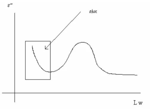
(7) 231. FUNDAMENTALS AND APPLICATIONS OF DEA. Figure 5. Argand diagram for a polymer following Havriliak- Negami equation. Up to now, we have considered only dielectric contributions. However, there is the phenomenon of conductivity that can overlap with dipole relaxation measurements of ε´ and ε´´. When an electric field is applied on a dielectric material the free charges in it were originating an energy loss that contributes to ε´´ value. ε´´=εdip+σ/ε0w. (13). where σ is the bulk ionic conductivity. The contribution of the conductivity[7] reflects as a substantial increase in ε´´, as shown in Fig. 6 and in Fig. 7.. Figure 6. Argand diagram for conductive component materials. a > b > c >d..

(8) 232. LISARDO NÚÑEZ, CARLOS GRACIA-FERNÁNDEZ, SILVIA GÓMEZ-BARREIRO. Figure 7. Plot of ε´´ versus Lw for a dielectric material. It is important to point out that the ionic conductivity also affects ε´ as free charges can accumulate on the electrodes thus changing the value of the permittivity as measured by the experimental equipment. Kohlrausch[8], and Williams and Watt[9] gave an expression for φ(t): φ (t ) = (e −t / τ ) β (14) with 0 ≤ β ≤ 1. The use of this equation as it happens with Cole-Davison and Havriliak-Negami gives an asymmetric Argand diagram closely related to the asymmetry of the relaxation times distribution function. In general, the data obtains must be analysed through an Argand plot, at a fixed temperature, observing which equation fits better the experimental results. 4.2.. Temperature domain. Temperature has a very strong influence on the dielectric behaviour of a material. Because of this, it is very important to know the relationship between frequency and temperature. For a dynamic experiment at a given frequency, in which the sample is heated at a constant rate, the transition temperature is taken either as that corresponding to the maximum of the ε´´ vs T curve or that corresponding to the maximum of the tan δ vs T plot. In the particular case of the glass transition, the transition temperature is designed as Tg. A simple relationship between f and T is the Arrhenius-like equation: −. Ea. f = f 0e RT (15) where Ea is the activation energy, R the gas constant and f0 a factor. This equation simulates correctly the behaviour of polymer transitions at temperatures below Tg. However, the temperature dependence for the α relaxation in amorphous polymers is usually found to follow the Vogel-Fulcher[10,11] equation:.

(9) FUNDAMENTALS AND APPLICATIONS OF DEA. −. 233. B. f = Ae T −T0 (16) where A, B and T0 are constants for a given material. Experimentally, it is found that T0 values are in the range between 30 and 70 ºC below the Tg value as measured by DSC. Both Arrhenius and Vogel-Fulcher equations can be used either as functions of the frequency or of its reciprocal the relaxation time. In this case, the Eqs.(15, 16) can be written as: Ea. τ = τe RT. (15 bis). B T − T0. τ = Ae (16 bis) Williams, Landel and Ferry[12] relate the variable studied to reference value, obtaining from Eq. (16 bis) the following expression, known as the WLF equation: τ − C1 (T − Ts ) (17) Ln = τ s C2 + T − TS where C1 = B / T-T0 and C2 = T-T0. Sheppard and Senturia[13] used this equation to study epoxy systems. Values reported for C1 are in the range between 14 and 18 while C2 values fall in the range 3070. Once of the most important applications of WLF is the construction of master curves [14] based on the time- temperature superposition principle. Experimental frequency and temperature data are usually represented in the form of an ln f vs 1000/T(K) Arrhenius plot. For sub-Tg transitions, Ea can be obtained from the slope of the straight line plot. However, for amorphous polymers, the plot strongly curves as Tg increases following WLF equation. 5. Practical applications to a cured thermoset. As a practical application[15,16], a study on the cured system DGEBA/mxylilenediamine is made. The system has been subjected to two types of temperature programs. One of them consisted of ramps every 2 ºC and keeping the temperature constant for a time that allowed a frequency scanning in the range between 10-1 to 106 Hz. This ensures that the measurements of ε´ and ε´´ have been carried out at the same constant temperature. These experiments are known as isothermal experiments. In the second type of experiments, known as dynamic ones, the temperature is increased at a constant rate of 2 ºC/min. Fig. 8 and 9 show ε´ and ε´´ respectively as functions of temperature in dynamic experiments at 2 ºC/min, carried out in the range between –150 and 280 ºC..

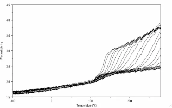
(10) 234. LISARDO NÚÑEZ, CARLOS GRACIA-FERNÁNDEZ, SILVIA GÓMEZ-BARREIRO. Figure 8. ε´ as a function of temperature for the system DGEBA (n = 0)/ m-XDA.. Figure 9. ε´´ as a function of temperature for the system DGEBA (n = 0)/ m-XDA.. Fig.8 shows the typical behaviour of an amorphous crosslinked network, in which a gradual increase in temperature originates different transitions thus causing an increase in ε´. This increase is originated by the increasing motion that temperature causes in dipoles allowing them to align with the applied field. It must be pointed out that the dipole orientation capacity depends on the field frequency..

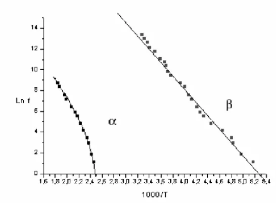
(11) FUNDAMENTALS AND APPLICATIONS OF DEA. 235. As the frequency increases the dipole orientation needs increasing temperatures. The different transition are observed as peaks in the ε´´ - T curve. The transition at the higher temperature is known as the α- transition and is related to the material glass transition. This is the reason why Tg is taken as the maximum value in a ε´´ - T curve. The transition at the lower temperature is named the β-transition and is associated to the motion of the side chains. In Fig.9 it can be observed also an increase in the mobility of the ions in the sample. Fig. 10 is an Arrhenius plot for the α and β transitions of the epoxy system studied. It shows a linear behaviour of the β-transition while the α-transition presents a curvature with changes in the slope. This relaxation follows a Vogel equation behaviour. At temperatures high enough, both transitions can overlap originating the αβ transition. In our case, this behaviour does not take place because the system is unable to reach high temperatures without degradation processes.. Figure 10. Arrhenius plot of the α and β transitions of the thermoset BADGE(n=0)/mXDA.. The apparent activation energy corresponding to the β-transition is, in this case, 67kJ/mol. WLF equation was used to calculate C1 and C2 values that characterizing the α-transition resulting C1=16.2 and C2=62.0..

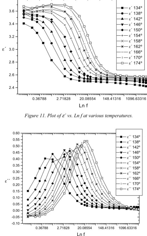
(12) 236. LISARDO NÚÑEZ, CARLOS GRACIA-FERNÁNDEZ, SILVIA GÓMEZ-BARREIRO. For the analysis of the isothermal experiments of the cured system, plots of ε´ and ε´´ vs. T were constructed (Figs. 11 and 12) at temperatures close to the α-transition determined through dynamic experiments. 3.8. ε´ ε´ ε´ ε´ ε´ ε´ ε´ ε´ ε´ ε´ ε´. 3.6. 3.4. 3.2. ε ´ 3.0 2.8. 134º 138º 142º 146º 150º 154º 158º 162º 166º 170º 174º. 2.6. 2.4 0.36788. 2.71828. 20.08554. 148.41316. 1096.63316. Ln f. Figure 11. Plot of ε´ vs. Ln f at various temperatures.. 0.60. ε´´ 134º ε´´ 138º ε´´ 142º ε´´ 146º ε´´ 150º ε´´ 154º ε´´ 158º ε´´ 162º ε´´ 166º ε´´ 170º ε´´ 174º. 0.55 0.50 0.45 0.40 0.35 0.30. ε´´. 0.25 0.20 0.15 0.10 0.05 0.00 -0.05 -0.10 0.36788. 2.71828. 20.08554. 148.41316. 1096.63316. Ln f. Figure 12. Plot of ε´´ vs. Ln f at various temperatures..

(13) FUNDAMENTALS AND APPLICATIONS OF DEA. 237. In Fig. 11 it can be seen that ε´ decreases with increasing frequencies. The reason is that the dipoles can not follow frequency from a given value. This decrease in ε´ is related to a peak in the ε´´ vs. Lnf plot. (see Fig. 12) Fig. 13 is an Argand diagram, that is a plot of ε´´ vs. ε´ at different temperatures. It can be seen that the plot does not correspond to a semicircle with center on the x-axis. For this reason, experimental data will be fitted to H-N equation. Real and Imaginary parts of the complex permittivity where plot separately in Figs. 11 and 12. Fitting to HN equation allows calculation of parameters a, b, εu, εr, τ and σ that supply important information about system relaxation.. Figure 13. Argand plot for the thermoset BADGE(n=0)/m-XDA at 134, 154 and 174 ºC. 6. Application of DEA to thermoset cure processes.. Characterization of a cured thermoset by DEA and the information available from this type of measurement, have been reported earlier in this chapter. It must be pointed out the great amount of papers reported[15,16] on the way to optimize DEA data with the objective of obtaining important information on the behaviour of this kind of systems. In our opinion, the study of thermosets during the cure processes[17-23] is, perhaps, more important due to the technological necessity of knowing the fundamental properties of the mixture to optimize the final product. This is the reason why many investigators have focused on the characterization of the cure process through DEA trying to relate dielectric properties to mechanical, rheological and mainly thermodynamical properties. This was facilitated by the increase and improvement of TA equipment and among them, DEA. In our study a DEA 2970 of TA instruments was used. The study of a curing process increases the complexity of the system since dielectric properties depend totally on temperature time and cure degree as well as on form and chemical composition of the substances involved in the mixture. Because of.

(14) 238. LISARDO NÚÑEZ, CARLOS GRACIA-FERNÁNDEZ, SILVIA GÓMEZ-BARREIRO. this, one the most used experiment is the isothermal (constant temperature). Figs. 14 a)c) are plots of permittivity, loss factor and ionic conductivity as functions of time. They correspond to the isothermal cure of the system DGEBA(n=0)/1,2 DCH at 55 ºC in the frequency range from 10-1 to 105 Hz.. Figure 14. a) ε´ as a function of time for the isothermal (55 ºC) curing process of the system DGEBA/1,2 DCH. Frequencies decrease with increase time.. Figure 14. b) ε´´ as a function of time for the isothermal (55 ºC) curing process of the system DGEBA/1,2 DCH. Frequencies decrease with increase time..

(15) FUNDAMENTALS AND APPLICATIONS OF DEA. 239. Figure 14. c) σ as a function of time for the isothermal (55 ºC) curing process of the system DGEBA/1,2 DCH. Frequencies decrease with increase time.. Fig. 14 a) shows that permittivity slightly decrease with time, at short times or high frequencies. This is the so called relaxed permittivity (εr) that can be only observed at high frequencies because at low frequencies, conductivity is high enough to cause electrode polarization[24], characterized by the extremely high values of ε´ at low cure times. εr measures the molecular dipole contribution that decreases with time owing to the chemical changes originated during the curing process. Increasing the curing time, ε´ undergoes a significant decrease originates by the vitrification of the system that make molecular dipoles unable to orientate with the electric field and unable to contribute to the real permittivity of the system. This decrease will take place at shorter times as the measurement frequency increases. Once the cure reaction has proceed, the permittivity tends to a constant value known as the unrelaxed permittivity (εu) to which only atomic and electronic polarizability contribute. The difference εr-εu is known as the dipole strength represented by Δε that is directly related to molecules dipole contribution. Because of this, the variation of Δε with time in isothermal conditions provides information about the changes in molecular dipoles originated by the chemical reactions during the cure process. Even DEA supplies information on dipole density and moment, there are some other techniques that provide more reliable information about the molecular configuration. For instance, infrared spectroscopy is a very strong technique to determine concentration of primary, secondary and tertiary amines during the curing reaction of an epoxy diamine system. A plot of ε´´ vs. t is shown in Fig. 14 b. As it was previously mentioned, there are two phenomena that contribute to ε´´: ionic conductivity and dipole relaxation. In the case of cured thermosets, conductivity is only significant at temperatures considerably above Tg and because of that, does not affect on the observation of that transition. However, in the case of the curing reaction, conductivity is a dominant.

(16) 240. LISARDO NÚÑEZ, CARLOS GRACIA-FERNÁNDEZ, SILVIA GÓMEZ-BARREIRO. factor, mainly at low curing times and frequencies, that sometimes hides the vitrification process. Fig. 14 b shows also that the loss factor decrease significantly with an increase in curing time. In this zone, the values of ionic conductivity are higher so the conductivity makes an important contribution to ε´´. The marked decrease in ionic conductivity with time is originated by an increase in the viscosity of the system and because of that, in the decreasing of the free volume caused by crosslinking of the system. The time to reach infinite value for viscosity is known as the gel time (tgel). Johari25 proposed an equation that relates ionic conductivity (σ), with cure time (t) ant tgel as follows: x. §t −t · σ = σ 0 ¨ gel ¸ (15) ¸ ¨ t © gel ¹ Where σ0 is the conductivity at t=o and x is a critical exponent depending on the isothermal cure temperature. The value of tgel can be obtained approximately from this equation in an isothermal cure. As the cure time increases, ε´´ increases due to vitrification and the ε´´-t curve presents a maximum at a given time. Same as it happened with ε´, the time corresponding to the maximum of the curves depends on the frequency, with higher values at low frequencies. If we want to obtain the time to vitrification, we have the problem that thus kind of dynamic measurement depends on frequency. Some authors propose that the time to vitrification coincides with the time to reach the maximum of the ε´´ vs. t curve at frequencies in the range from 1 to 3 Hz. Because there are two phenomena that contribute to ε´´, it may happen that at low frequencies, dipole transition is overlapped by the ionic contribution as it happens in Fig. 14b. For this reason, the experimental procedure must be careful, trying to attain maximum resolution for vitrification minimizing the conductivity contribution. As the reaction progress, ε´´ tends to a constant value that depends greatly on the ionic conductivity or the system after being cured. A practical way to check, at a given reaction time, which of the two phenomena, dipole or conductivity, is dominant, is based on the plot of σ (ε´´wε0) versus time at different frequencies (Fig. 14 c) because the conductivity contribution does not depend on the frequency. It can be seen in Fig. 14 c that, at first stages of curing, ionic conductivity is the most important contribution to ε´´ and decreases with time. At higher curing times, σ depends on frequency, thus indicating that the system is in the vitrification zone where dipole relaxations depend on w. At high curing times, the curing reaction is complete for the isothermal temperature and ionic conductivity becomes dominant. There were different attempts to relate dielectric measurements with some other thermal analysis techniques especially with calorimetric measurements as they were frequently used and provide important information. The cure degree α was related to conductivity through the following equation: 1 ∂ log σ = ∂α (16) ∂t ∂t ∂α where 1/σ is the resistivity of the system and , the reaction rate. ∂t.

(17) FUNDAMENTALS AND APPLICATIONS OF DEA. 241. Maffezzoli[19] proposed an equation that relates α and σ:. log σ 0 − log σ α = α max log σ 0 − log σ ∞. P. § log σ ∞ · ¨¨ ¸¸ (17) © log σ ¹ is the conversion at the end of the isothermal cure and p is an. where αmáx empiric parameter. Interpretation of experimental data becomes more complicated when introducing a new experimental variable: temperature. When the resin-hardener mixture is subjected to an increase in temperature at a controlled heating rate, both ε´ and ε´´ depend on time, temperature and cure degree. A quantitative analysis of this type of experiments is represented in Fig. 15. This Figure shows the behaviour of a epoxy resin-aliphatic diamine system when mixture is subjected to a controlled heating rate at 5 ºC/min. One of the most useful variables for graphical representation of this kind of experiments is the logarithmic of ionic conductivity. As in the case of isothermal experiments, it allows to differentiate between zones in which conductivity is dominant (and because of this vitrification or glass transition does not exist) and zones in which dipole transitions are dominant.. Figure 15. Plot of σ vs. T for an epoxy-diamine system.. Fig. 15 shows that at low temperatures (from -100 to 0 ºC), ionic conductivity depends on frequency and the glass transition proceed without reaction (Tg0). As the temperature increases, conductivity increases up to a value that corresponds to a minimum in viscosity. It must be pointed that ionic conductivity can be divided into two different contributions: - a thermal component, which increases as temperature increases (simple fluidification). This term σth can be analysed as a thermal agitation contribution on σ; - a curing component, which increases resin molecular weight and then viscosity. By this way, molecular mobility decreases. This term σcure leads to a decrease in σ. Precisely, this second term is the cause of the ionic conductivity decrease when the temperature increase because there is an approach to gelation of the system in wich.

(18) 242. LISARDO NÚÑEZ, CARLOS GRACIA-FERNÁNDEZ, SILVIA GÓMEZ-BARREIRO. viscosity tends to infinite (see that there is not dipole contribution in the range from 25 to 75 ºC because σ does not depend on frequency). If the temperature goes on increasing, the process becomes again dipole motion controlled. Vitrification takes place and at greater temperatures glass transition. As both processes depend on frequency, at low frequencies they overlap, as it can be seen in Fig. 15. Vitrification an glass transition peaks are clearly differentiated at 105 Hz. A further increase in temperature originates an increase of conductivity in the rubber state of the system. Let us to consider some practical cases of the use of DEA for characterization of polymeric materials. 7. Characterization of Ethylene Vynil Acetate Copolymers by Dielectric Analysis. (Courtesy of TA Instruments). Ethylene-Vinyl acetate (EVA) is a generic name used to describe a family of thermoplastic polymers ranging from 5 to 50% by weight of vinyl acetate incorporated into an ethylene chain. Increasing the level of vinyl acetate in EVA polymer reduces the overall crystallinity level associated with the polymer, which increases its flexibility and reduces its hardness. A series of EVA polymers, with varying levels of vinyl acetate was analyzed using the Dielectric Analyser 2970 with the ceramic single surface sensor. The EVA polymers contained the following levels, by weigth, of vinyl acetate; 14, 18, 25, 28 and 33%. To directly compare results between samples, therefore, a single frecuency which yields a well-defined loss peak must be chosen. Figure 16 is the comparative data at 1000 Hz. The comparative plots shows that the glass transition temperature is relatively insensitive to the level of vinyl acetate in the EVA polymer. However, the magnitude of the loss transition is very dependent on the concentration of vinyl acetate. As the level of vinyl acetate increases, the magnitude of the loss factor peak increases. This is consistent with the fact that increasing the level of vinyl acetate increases the flexibility associated with the polymer. Hence, a DEA analysis based on calibration with a series of known EVA formulations could be used to follow vinyl acetate content.. Figure 16. Comparative plot of ε´ vs. T for different levels of vinyl acetate..

(19) FUNDAMENTALS AND APPLICATIONS OF DEA. 243. 8. Characterization of PMMA by Dielectric Analysis. (Courtesy of TA Instruments).. Poly (methyl methacrylate), or PMMA, is a thermoplastic material commonly used in applications where good impact properties are required. The mechanical properties exhibited by PMMA are due, in part, to the occurrence of a secondary transition (beta relaxation) near room temperature. The sintered powder was heated at a rated of 3 ºC/min from -80 to 180 ºC .The following analysis frequencies were utilized: 1, 3, 10, 30, 100, 300, 1000, 3000 and 10000 Hz. Displayed in Figure 17 are the results (loss factor, ε´´) for the PMMA specimen. The beta transition, which is associated with the rotation of the methacrylate group, is observed as a series of peaks between 0 and 100 ºC. The transition is frequency dependent since it is a time-dependent, nonequilibrium event. The alpha or glass transition occurs at approximately 120 ºC. This event is also frequency dependent. The loss factor data reveals that, at the lower frequencies, the two transitions are clearly resolved and two separate peaks are observed. As the applied frequency increases, the resolution between the alpha and beta events decreases. This observed behaviour is expected for two transitions which occur relatively close to one another and have significantly different activation energies.. Figure 17. Plot of ε´´ vs. T for PMMA at different experimental frequencies. References. 1. 2. 3. 4. 5.. J.M. Albella, J.M. Martínez: Física de Dieléctricos (Marcombo Boixareu Editores, Barcelona México). P. Debye: Polar Molecules (Chemical Catalog Co., New York 1929) K.S. Cole and R.H. Cole: J. Chem. Phys. Vol. 9 (1941), p. 341 D.W Davidson, R.H.J. Cole: Chem. Phys. Vol. 19 (1951), p. 1484 S. Jr. Havriliak, S.J. Negami: Polymer Sci. Vol 14 (1966),p. 99.

(20) 244. 6. 7. 8. 9. 10. 11. 12. 13. 14. 15. 16. 17. 18. 19. 20. 21. 22. 23. 24.. LISARDO NÚÑEZ, CARLOS GRACIA-FERNÁNDEZ, SILVIA GÓMEZ-BARREIRO. S. Jr. Havriliak, S.J. Negami: Polymer Vol 8 (1967),p. 161 S. D. Senturia, N. F. Sheppard: Dielectric Analysis of thermoset cure (SpringerVerlag, Berlin Heidelberg 1986). R. Kohlausch: Anu. Phys. Chem Vol 91 (1854), p. 179 G. Williams, D.C. Watts: Trans Faraday Soc Vol 66 (1970), p. 80 H. Vogel: Physik Z. Vol 22 (1921),p. 645 G.A. Fulcher, J. Am. Cerm. Soc. Vol 8 (1925),p 339 M. L. Williams, R. F. Landel and J. D. Ferry: J. Am. Chem. Soc. Vol 77 (1955),p. 3701 N. F. Sheppard, S. D. Senturia: Journal of Polymer Science Vol 27 (1989),p. 753 J. D. Ferry: Viscoelastic Propierties of Polymers (John Wiley & Sons, New York 1993) M. Matsukawa, H. Okabe, K. Matsushigto: Journal of Applied Polymer Science Vol 50 (1993),p. 67 M. Ochi, M. Yoshzumi, M. Shimbo: Journal of Applied Polymer Science Vol.25 (1987),p. 1817 J. T. Gotro, M. Yandrasits: Polym. Eng. Sci. Vol. 29 (1989),p. 278 J. O. Simpson, Bidstrup : Polym. Mater. Sci. Eng. Vol. 65 (1991),p. 339 A. Maffezolli, A. Trivisano, M. Opalicki, J. Mijovic, J.M. Kenny : J. Mater. Sci Vol. 29 (1994),p. 800 S. Montserrat, F. Roman, P. Colomer ; Polymer, 44, 101, (2003). M.B.M. Mangion, G.P. Johari, J. Polym. Sci.: Polym.Phys. Edn., 28, 1621 (1990). M.B.M. Mangion, G.P. Johari, Macromolecules., 23, 3687 (1990). M.B.M. Mangion, G.P. Johari, J. Polym. Sci.: Polym.Phys. Edn., 29, 437 (1991). M.B.M. Mangion, G.P. Johari, J. Non Crystaline Solids, 133, 921 (1991)..

(21)