Department of Physics and Astronomy, University of Pittsburgh, Pittsburgh, PA 15260, USA 8
Cerro Tololo Inter-American Observatory, National Optical Astronomy Observatory, Casilla 603, La Serena, Chile 9Department of Astronomy, University of Washington, Box 351580, Seattle, WA 98195-1580, USA 10
Aix Marseille Université, CNRS, LAM(Laboratoire dÁstrophysique de Marseille)UMR 7326, F-13388, Marseille, France 11
Pontificia Universidad Catolica de Chile, Instituto de Astrofisica, Casilla 306, Santiago 22, Chile 12
Department of Astronomy, University of Virginia, Charlottesville, VA 22904-4325, USA 13
School of Mathematics and Physics, University of Queensland, Brisbane, QLD 4072, Australia 14
Department of Astronomy, 601 Campbell Hall, University of California, Berkeley, CA 94720-3411, USA 15
Department of Physics, University of Notre Dame, 225 Nieuwland Science Hall, Notre Dame, IN 46556-5670, USA 16
Department of Physics and Astronomy, Rutgers, The State University of New Jersey, Piscataway, NJ 08854, USA 17
Department of Physics and Astronomy, Texas A & M University, College Station, TX 77843-4242, USA 18
European Southern Observatory, Karl-Schwarzschild-Strasse 2, D-85748 Garching, Germany 19
Fermilab, P.O. Box 500, Batavia, IL 60510-0500, USA
20Departamento de Ciencias Fisicas, Universidad Andres Bello, Avda. Republica 252, Santiago, Santiago RM, Chile 21
Astronomy Nucleus, Faculty of Engineering, Universidad Diego Portales, Ejército 441, Santiago, Santiago RM, Chile 22
Johns Hopkins University, 3400 North Charles Street, Baltimore, MD 21218, USA 23
Department of Astronomy, University of Texas, Austin, TX 78712-0259, USA 24
Oskar Klein Centre, Department of Astronomy, AlbaNova, Stockholm University, SE-10691, Stockholm, Sweden 25
Institute for Astronomy, University of Hawaii, 2680 Woodlawn Drive, Honolulu, HI 96822, USA 26
Millennium Institute of Astrophysics, Chile
Received 2015 May 26; accepted 2015 December 22; published 2016 May 6
ABSTRACT
The ESSENCE survey discovered 213 Type Ia supernovae at redshifts0.1< <z 0.81between 2002 and 2008. We present theirR-andI-band photometry, measured from images obtained using the MOSAIC II camera at the CTIO Blanco, along with rapid-response spectroscopy for each object. We use our spectroscopic follow-up observations to determine an accurate, quantitative classification, and precise redshift. Through an extensive calibration program we have improved the precision of the CTIO Blanco natural photometric system. We use several empirical metrics to measure our internal photometric consistency and our absolute calibration of the survey. We assess the effect of various potential sources of systematic bias on our measuredfluxes, and estimate the dominant term in the systematic error budget from the photometric calibration on our absolutefluxes is∼1%.
Key words:cosmology: observations –methods: data analysis –supernovae: general–surveys
1. INTRODUCTION
We present the calibrated photometry of 213 Type Ia supernovae (SNIa) measured by the Equation of State: Supernovae trace Cosmic Expansion (ESSENCE) survey between 2002 and 2008. Our report more than doubles the sample presented by Miknaitis et al. (2007)and Wood-Vasey et al.(2007). We have made a significant effort to improve the photometric calibration of the survey. As ESSENCE observed in only two passbands, our measurements of luminosity distance are strongly correlated with extinction in the host galaxy of the SNIa and arevery sensitive to the systematic error budget from photometry. In particular, the light curves in this work are computedusing data taken only with the 4 m
Blanco Telescope at the Cerro Tololo Inter-American Obser-vatory, eliminating cross-telescope systematics present in the calibration by Miknaitis et al. (2007). A companion work (B. E. Tucker et al. 2014, in preparation) will report on properties of the host galaxies of our SNIa sample. In future work, we will use this sample along with low-redshift SNIa from the literature to perform a full cosmological analysis and improve constraints on the nature of the dark energy.
Since the discovery of the luminosity–width–color relation (Phillips1993), SNIa have been our most precise standardiz-able candles at cosmological distances. The initial Calán-Tololo sample of 29 SN in 4 colors (Hamuy et al. 1996) enabled the development of various algorithms capable of correcting the dispersion in the intrinsic brightness of SNIa, and inferring the luminosity distances to ∼10% per object
27
(Riess et al.1996; Phillips et al.1999; Goldhaber et al.2001). These light curve fitters have been refined as the size of the nearby sample has increased and its photometric precision has improved; current algorithms can determine the luminosity distance to wellobserved SNIa to∼5%(Guy et al.2007; Jha et al.2007; Conley et al.2008; Mandel et al.2011).
The distance moduli derived for these SNIa indicated that the universe is accelerating (Riess et al. 1998; Perlmutter et al. 1999). SNIa observations have remained our most sensitive cosmological probe of the expansion history. The accelerating expansion has been modeled by introducing afluid with negative pressure, called the dark energy, into the Friedmann equation: ais the scale factor, andΩis the total energy density of matter (M), photons (ν), curvature (k), and the dark energy (DE), respectively. Several groups have focused on measuring the ratio of pressure to density—the equation of state of thisfluid,
r =
w P ( c2)—to distinguish between different models of the
dark energy.
High-redshift SNIa surveys(Riess et al.2007; Wood-Vasey et al. 2007; Guy et al. 2010; Betoule et al. 2014; Sako et al. 2014) have independently reported measurements of w
consistent with −1, in good agreement with a classical cosmological constant. However, despite the rapidly growing number of SNIa, the precision of the measurement of whas stubbornly remained at the 10% level, dominated by various sources of systematic uncertainty. Several groups have attempted to reduce the effect of systematic errors in SNIa measurements on the dark energy figure of merit (FoM; Al-brecht et al.2006), by either incorporating new sources of data, or improving the calibration of existing data.
Early work by Krisciunas et al. (2000) demonstrated uniformity in the evolution of near infrared (NIR) colors of SNIa, and the potential of NIR measurements for cosmology (Krisciunas et al. 2004). Using increasingly large and better calibrated samples of nearby SNIa with JHKs measurements,
Wood-Vasey et al. (2008), Mandel et al. (2009), and Barone-Nugent et al. (2012) have shown that the NIR light curves of SNIa span a smaller range in luminosity than in the optical. Because distance moduli derived from NIR measurements are less susceptible to host galaxy dust absorption, the residual scatter in a Hubble diagram generated from infrared light curves alone is comparable to the scatter derived from light-curve-shape-correctedoptical data. Consequently, high-zsurveys have increasingly attempted to probe further into the rest-frame infrared. Freedman et al. (2009)presented the first IR Hubble diagram toz∼0.7, but were limited by a relatively small sample size, systematic uncertainties in their photometric calibration, and the difficulty of obtaining IR data at high-z, where it is redshifted to even longer wavelengths. Future high-redshift surveys, such as RAISIN (R.P. Kirshner—Hubble Space Telescope (HST)Proposal 13046), will provide valuable high-redshift SNIa measurements that probe the rest-frame NIR.
Kelly et al.(2010)illustrated that in addition to demographic differences between SNIa from passive and star-forming hosts, the Hubble diagram residuals are correlated with derived host galaxy size and stellar mass. This correlation indicates that the empirical luminosity shape relations employed by SNIa light
curve fitters do not fully account for the spread in intrinsic luminosity. In an effort to reduce this dispersion, Lampeitl et al. (2010) employed a simple linear correction based on host galaxy stellar mass and found an improvement in statisticalfit to the SNIa measurements. Sullivan et al.(2010)used different SNIa absolute magnitudes for high- and low-mass hosts in their cosmologicalfits and found a significant improvement in c2over using a relation expressed as a function of host galaxy
stellar mass.
However, although metallicity, extinction properties, and specific star formation rate correlate with host galaxy mass, the fundamental relation underlying this correlation with SNIa luminosity is not well understood. These relations may be an artifact of the treatment of SNIa color by light curve fitters; Scolnic et al.(2014a)found that the strength of correlation of the host galaxy properties with Hubble residual was reduced by
∼20% when SNIa are treated as having an intrinsic color scatter for a fixed luminosity distance, rather than an achromatic scatter in peak luminosity. In addition, there are challenges in deriving host galaxy properties from broadband optical photometry at high redshift in a manner that does not introduce additional systematic uncertainty into SNIa mea-surements. ESSENCE has undertaken a significant effort to determine host galaxy morphology and properties for our sample, to appear in B. E. Tucker et al.(2014, in preparation). Several authors (Wang et al. 2009; Blondin et al. 2011; Foley & Kasen2011; Nordin et al.2011; Walker et al. 2011; Silverman et al. 2012) have found that measurements from spectra of SNIa correlate with the residual intrinsic color dispersion after light curve shape correction. They furtherfind that these measurements, typically derived from pseudo equivalent widths of Ca or Si, can be used to improve the precision of distance moduli, although Blondin et al. (2011)
find that the improvement is not statistically significant(<2σ). While promising, this approach is limited by the need for high signal-to-noise ratio(S/N)spectra of SNIa. Additionally, the dependence on measuring the SiII6355 Å feature limits its use at high-z, where the redshifted Si features are often not covered by the high-throughput, low-dispersion spectrographs used by SNIa surveys.
Surveys such as ESSENCE, the Supernova Legacy Survey (SNLS), theSloan Digital Sky Survey (SDSS), and the Panoramic Survey Telescope and Rapid Response System (Pan-STARRS)have now produced well over a thousand well sampled SNIa light curves that span the redshift range over which the transition from cosmic deceleration to acceleration occurred. The crucial measurement for characterizing the nature of dark energy is mapping out luminosity distance versus redshiftto constrain the parameters of Equation(1). The precision of photometric calibration is now the dominant term of the SNIa survey systematic error budget. Wood-Vasey et al. (2007)found that systematic uncertainties from the photometry alone could lead to an ∼4% change in w. Exploiting the improved statistics from these large samples requires a corresponding improvement in the photometric calibration across diverse instruments, detectors andfilters.
various stages of implementation by Pan-STARRS (Tonry et al. 2012; Rest et al. 2014), SNLS (Regnault et al.2009), the joint efforts of SDSS and SNLS(Betoule et al. 2013,2014), andthe Dark Energy Survey (DES) and the Large Synoptic Survey Telescope(LSST). While the first method is well established, SNIa surveys require a higher level of precision than is possible with existing standard star networks. The second method is still nascent, and systems to measure the atmospheric component of the throughput are under active development(Albert et al. 2014). No purely laboratory-standard-based magnitude system yet exists. Several surveys, including ESSENCE, have elected to use a combination of both methods; thefirst to determine the absolute flux calibration, and the second to determine precise relative system throughputs.
Kessler et al. (2009)demonstrated that measurements of w
are extremely sensitive to the calibration of theUband at low redshift: inclusion of rest-frame U-band data at all redshifts causes a 0.12 mag shift in distance moduli, corresponding to an enormous 0.3 change in the equation of state parameter,w. The
U-band anomaly might arise from differences between the spectral energy distribution(SED)of SNIa that correlate with host galaxy properties or between objects at low and high redshift(Foley et al.2012; Maguire et al.2012). Additionally,
U-band measurements of the same nearby SNIa from different telescopes often exhibit differences that are inconsistent with the stated photometric uncertainties and system throughput measurements. Krisciunas et al.(2013)have demonstrated that careful modeling of the U-band transmission with appropriate
S-corrections can resolve the differences between SNIa measurements. The size of the systematics associated with the U-band, however, has led most high-z surveys to down weight, or discard rest-frame UV observations.
Larger, more precisely calibrated nearby samples( Ganesha-lingam et al.2010; Stritzinger et al.2011; Hicken et al.2012), along with better calibration of high-zSNIa surveys, offer the most direct path to reducing the systematic uncertainty on the equation of state parameter of the dark energy. Wide-field deep surveys such as Pan-STARRS and DES will obtain SNIa measurements over 0< <z 1.2 (Rest et al. 2014), further reducing systematic uncertainties from photometry by avoiding any errors associated with cross-telescope calibration and weakening the sensitivity of w to the overall photometric calibration of the survey (Scolnic et al. 2014b). Recognizing the need for precision calibration to reduce systematics(Stubbs
to obtain <1% photometry over much of the sky (Stubbs et al.2010; Schlafly et al.2012; Tonry et al.2012). This work details the calibration of the ESSENCE survey, with a focus on minimizing the systematic error budget from photometry.
We provide a brief overview of the ESSENCE survey in Section 2, followed by our photometric data reduction and calibration in Section 3. We discuss our spectroscopic followup and classification is Section 4. We illustrate our SNIa light curves, compare and contrast our methodologies for light curve fitting, and detail the properties of the full ESSENCE six-year sample in Section5. Our photometric error budget from various sources with systematic uncertainty is detailed in Section 6. We conclude in Section 7. The appendices contain further information on the computation of illumination corrections, the properties of the CTIO Blanco natural magnitude system employed in this work, tables containing the photometry of ESSENCE SNIa and likely SNIa without spectroscopic confirmation (hereafter, “Ia?”) objects during the year of discovery, and light curve fit parameters using the two most common methodologies.
2. THE ESSENCE SURVEY
Previous ESSENCE publications have described the survey strategy, fields, data processing (Miknaitis et al. 2007, hereafter M07), spectroscopic selection criteriaand follow up (Matheson et al. 2005; Foley et al. 2009), performed a preliminary cosmological analysis (Wood-Vasey et al. 2007, hereafterWV07), and scrutinized exotic cosmological models (Davis et al.2007). The SNIa search was carried out on the CTIO 4 m Blanco telescope(hereafterBlanco)over 197 half-nights in dark and graytime between September and January from 2002 to 2008. Science images were obtained using the 64 Mega pixel MOSAIC II camera with an Atmospheric Dispersion Corrector (ADC) through two primary filters (denotedR and I) similar to CousinsRC and IC. The field of
view of the system is 0.36 deg2on the sky at the f 2.87prime focus.
The survey covered a set of four primary fields (listed in Table 1, together with the number of times each field was observed), each consisting of eightsub-fields, clustered spatially. Fields were selected to be equatorial but outside the Galactic and ecliptic planes, in regions with low Milky Way extinction and minimal IR cirrus, and with coverage from existing surveys(including SDSS, the NOAO Deep Wide-Field Survey, and the Deep Lens Survey)where possible. Thefields were spaced to ensure that science images could be taken at low airmass. Fields were divided into two sets and each set was imaged in bothfilters every other observing night, resulting in a typical cadence of fourdays. Science frames are exposed for 200 s in R and 400 s in I. The original I filter (NOAO code c6005) sustained significant damage on 2002 November 10, severely degrading the image quality ofI-band data in CCDs 1 and 2 (amplifiers 1–4). The filter was replaced on 2003 May 25. CCD 3 failed shortly before the start of the 2003 observing season, resulting in a 12.5% loss in efficiency until it was replaced in 2004.
Survey images were reduced at CTIO using the “ phot-pipe”pipeline developed for use on the CTIO Blanco by the SuperMACHO survey (Rest et al. 2005; Garg et al. 2007; Miknaitis et al. 2007) that operated contemporaneously with the ESSENCE survey. Each science image was calibrated and aligned with afixed astrometric grid. We subtracted a reference template for each field, constructed using deep images from previous observations. Point-spread function(PSF)photometry from the resulting difference image was combined to identify sources that had varied over multiple epochs, while eliminating sources of contamination such as difference image artifacts and diffraction spikes from saturated stars. With limited time for spectroscopic follow up observations, we were forced to employ various cuts and selection criteria in order to determine the most promising candidates.
The spectroscopic follow-up observations of ESSENCE candidates is described in Section 4. All candidates were visually inspected to classify them and obtain redshifts. We produced a preliminary reduction of all spectra in real time, using standard IRAF28 routines, and some custom IDL
routines to facilitate data processing for the various instru-ments. Estimates of the redshift and classification were obtained on site usingSNID (Blondin & Tonry 2007). When preliminary classifications were unclear, we relied on the experience of the observers to determine if additional spectro-scopic follow up was warranted. Fields containing candidates with a clear classification as SNIa were followed for the remainder of the observing season. Following survey opera-tions, all data were transferred, initially to the Hydra Computing Cluster maintained by the Smithsonian Institution, and later to the Odyssey Compute Clusterhosted by the Research Computing Group at Harvard University for the analysis presented in this paper. All data is also available through the NOAO archive.29
3. DATA REDUCTION
3.1. Image De-trending
The eight CCDs of MOSAIC II were read out in pairs, through two amplifiers per chip, by four Arcon controllers. The
cross-talk between the amplifiers is subtracted using thextalk
task from themscredpackage for IRAF. All CCD images are de-biased and trimmed and masking was applied to bad pixels and columns. The mask is propagated through all subsequent reduction stages.
All science images areflat-field-corrected using domeflats. Theseflats accurately corrected for pixel-to-pixel variations but large-scale variations were introduced as a result of uneven illumination of the dome screen and stray light paths in the optical system. While the precision obtained from dome flat images alone is suitable for many projects, we required higher precision for SNIa cosmology and strived to minimize potential systematic errors in our photometry. We therefore accounted for large-scale illumination variation by constructing an illumination correction from the science images, as described below.
We applied the nightly domeflat image to all science images to construct a temporary preliminary flattened image. The resulting images were masked to remove contamination from all astrophysical sources, normalized to have the same sky value, and then averaged. The derived calibration image was inverted, smoothed with a large kernel, and scaled to have a mean of unity. This illumination correction was applied to the domeflat images to take out residual large-scale gradients. The science images were reprocessed with thisfinalflat-field image. To estimate the night-to-night stability of the illumination correction, we took the ratio of the correction image between different nights of a single run—a period of time during which MOSAIC II was continuously mounted on the telescope, typically one lunation. We found that the gradient pattern (a representative example is shown in Figure1)was very stable within a lunar cycle. The standard deviation of the ratio without sigma clipping was typically less that 0.1%, and the absolute value of the maximum difference between the ratio and the average of the ratio image was<0.003. Therefore, on nights with few science images of sparsefields or with excess stray light—either from insufficient baffling or around full moon— we exploited the stability of the gradient pattern to estimate the illumination correction from nearby nights. This estimation and temporal stability of the illumination corrections is examined in further detail in AppendixA.
Surveys that use master flats constructed for each run are susceptible to systematic trends, such as long period variations in amplifier gain. By contrast, our procedure avoids such effects: science frames were normalized with nightly flat frames and primarily used illumination corrections determined from the same, or at the least extrapolated only from nearby, nights.
3.2. Astrometric Calibration
In order to construct difference images to search for and measure the flux of variable and transient objects, we first imposed a consistent astrometric solution and warped all the science images to a consistent pixel coordinate system. The transformation between the local image pixel coordinate system and the FK5 World Coordinate System is dominated by optical distortions that are well described by a low-order polynomial in radius from the field center. We determined the polynomial terms of the distortion function from images of dense LMC
fields using the IRAF task,msctpeak. The distortion terms were used in combination with theIRAFtaskmsccmatchto derive a WCS solution for eachfield. The distortion terms were
28
IRAFis distributed by the National Optical Astronomy Observatory, which is operated by AURA under cooperative agreement with the NSF.
29
six months. If left uncorrected, this variation would introduce systematic offsets at the∼0 01 level.
With the distortion modeled, the astrometric solution for any image with the equatorially mounted Blanco reduces to determining the linear rotation matrix with respect to the center. We used theIRAFtaskmscmatchfrom themscred package to match pixel coordinates for objects in the image to an existing catalog of the field with precise astrometry. We generated an initial astrometric solution for the survey using reference catalogs derived from the Sloan Digital Sky Survey DR7(Abazajian et al.2009)wherever possible, and defaulting to astrometry from the USNO CCD Astrograph catalog 2 (UCAC;Zacharias et al. 2004) where SDSS coverage was unavailable. As the SDSS is itself tied to the UCAC, and as we only require preciserelativeastrometric calibration to precisely position the PSF and measure flux, errors caused by the differences of the astrometric solution between the two different reference catalogs are negligible. We used this initial solution to generate secondary astrometric catalogs using our multiple observations of each field.
Finally, we used the astrometric solution and the SWarp
(Bertin et al. 2002) package to re-sample each image to a common pixel coordinate system using a flux-conserving, Lanczos-windowed sinc kernel. We generated weight maps for each image to account for the change in the noise properties produced by re-sampling. Some covariance between pixels is introduced as a result of the re-sampling process and we accounted for it during difference imaging.
3.3. Flux Measurement
We used the DoPHOT photometry package (Schechter et al.1993)to identify and measure sources within the warped images. DoPHOT is appropriate for point source photometry. B. E. Tucker et al. (2014, in preparation) will report on photometry of extended sources.
3.4. Photometric Calibration
High-redshift SNIa surveys typically report observations in their natural photometric system, relating magnitudes to measuredflux via:
f
= - +
mT i, 2.5 log10( ADU, ,T i) ZPT i,, ( )2
where m is the natural magnitude, f the measured flux, and ZPT i, is the instrumental zero point of the image, i, observed
through passbandT.
surveys to schedule observations in different passbands independently, as the SNIa colors at every epoch are not needed, and they avoid the additional photometric errors that arise from converting the observed supernovaflux to a standard system. These transformations are non-trivial, as the simple linear transformations derived for stars are not directly applicable to SNIa with their more complex SEDs. However, as these measurements are reported in a non-standard magnitude system, surveys must establish a network of stellar calibrators in the natural system of the telescope to derive accurate and precise zero points. In addition, an accurate model of the survey throughput in each passband is required so measurements in the natural system can be compared to synthetic fluxes generated from models derived from SNIa measurements at low-redshift in the standard system. We have developed various metrics to quantify our internal photometric consistency, and verified our zero point consistency using the SDSS. We detail the improvements to the photometric calibration for the survey in the next subsections.
3.4.1. Aperture Corrections
The extended aureole of astrophysical objects has a surface brightness profile that roughly followsr-2, and a large fraction
of theflux is outside the seeing disk. Thus, an aperture larger than the seeing disk is necessary for the enclosedflux to be a reliable estimator of the true sourceflux. However, the larger the aperture, the higher the error from sky subtraction, and the higher the probability of enclosing contaminating sources. We follow the standard technique of addressing this trade off by measuring the flux in a fixed aperture, and determining an aperture correction to correct for itsfinite size.
removed. If more than 25% of the stars were clipped, the aperture correction for the image was flagged “bad.” We checked that the growth curves asymptotically approached a constant value for all apertures larger than 22 pixels, and
flagged those that did not. We measured the total aperture correction to an aperture radius of 25pixels, or ∼13 5 in diameter, chosen to effectively enclose most of theflux of each object for all ESSENCE images, which have a typical FWHMof the PSF of∼1 2 in both passbands(see Figure3).
3.4.2. Choice of Standard Star Network and a Fundamental Spectrophotometric Standard
While several standard stellar catalogs report broadband magnitudes in different photometric systems through a range of passbands (Landolt 1983; Stetson 2000; Ivezić et al. 2007; Landolt & Uomoto2007), the standard star network of Landolt (1992), extended by Stetson(2005), remains the most obvious choice to tie to the Johnson-Morgan-Cousins photometric system. The RC and IC Cousins filters are broadly similar to
those used on the Blanco (see Figure 4), and the magnitudes reported by low-redshift SNIa surveys are converted into the Johnson system using observations of the Landolt network stars. This allows us to minimize systematic uncertainties when comparing our data to the nearby sample.
The choice of standard star network and the transformation equations derived between the natural and standard system also play a critical role in determining the absolute throughput of each passband. This calibration enables SED models of SNIa generated from low-redshift observations to be converted into the Blanco natural magnitude system via:
⎜ ⎟
⎛ ⎝
⎞ ⎠
ò
l l l l= - +
m F T
hc
2.5 log d ZP . 3
T 10 ( ) ( ) T ( )
This equation is inverted to determine the zero point, ZPT,
for the full optical system (detector, optics, filter, and atmosphere) with dimensionless total photon efficiency,
l
T( ), using a star with a well-measured SED,F( )l30, whose magnitudes, mT, are known in the natural system—a“
funda-mental spectrophotometric standard.”
Figure 2.Typical differential curves of growth forR(left, red)andI(right, orange)on 20071103, for amplifier 4(both randomly selected). The point at the smallest physical aperture is the difference between theDoPHOTmagnitude of the object and magnitude with an aperture radius of 5 pixels. We have used a piecewisey-axis scale to show the full range of the data without compressing local variations. We have plotted the individual isolated stars in gray. We offset each individual star slightly from the aperture through which theflux is measured along the-xdirection for clarity. We checked that the growth curve is consistent with a constant for apertures larger than 22pixels, indicated by vertical lines with an arrow in between. Errors in the average measurement at each aperture,dA, are typically smaller than the plot symbols. We propagated the covariance matrix between apertures to determine thefinal aperture correction at a radius of 25pixels(indicated with a blue star, and labeled in the left panel).
Figure 3.FWHM Distribution ofRandIscience images from the survey. The mean FWHM is 1 24 for theRband and 1 2 forI.
30
The formalism employed throughout this work represents SEDs as power per unit wavelength as a function of wavelength, while the system throughput is represented as a dimensionless photon efficiency. The former is typically provided in erg s−1cm−2Å−1. If the system throughput is provided in erg Å−1, then the extra factor of the inverse energy,l
hc, must be dropped to account for
Unfortunately, most well-measured spectrophotometric stan-dards are too bright to be measured directly by the Blanco. We must therefore infer the Blanco natural magnitudes of the fundamental standard using the star’s standard magnitudes. The most direct way of achieving this is to define the transformation equations such that the Landolt and natural system magnitudes agree at some color.
Historically, the choice for the fundamental standard for SNIa surveys has been αLyr(Vega), either implicitly when the rest-frame SNIa model is constructed from low-zdata, or explicitly, when defining the passband zero points for high-redshift surveys (Astier et al. 2006; Miknaitis et al. 2007; Hicken et al. 2009b, 2012; Contreras et al. 2010; Stritzinger et al.2011). Vega was one of sixA VÆ stars used to establish the color zero point on the photometric system of Johnson & Morgan(1953)by defining the meanU−BandB−Vcolors of the six to be zero, and this definition was further extended to Cousins RC -IC. Vega’s SED was tied to tungsten-ribbon
filament lamps and laboratory blackbody sources employed as fundamental standards (Oke & Schild 1970; Hayes & Latham 1975). With the widespread adoption of the Landolt standard star network to tie instrumental photometry to the Johnson system, the use of Vega as the fundamental spectro-photometric standard became ubiquitous.
However, as discussed by Regnault et al.(2009), Vega is far from an ideal choice for the fundamental standard. Taylor (1986)found that in order for several sources of synthetic and observed Cousins RC-IC measurements to agree, the IC
transmission curve had to be shifted to the red by 50–100 Å.
models are used to extend the observed SED of Vega into the UV and IR.
Following several groups including the SDSS (Ivezić et al. 2007)and the SNLS(Regnault et al. 2009), we instead select the sdF8 D star, BD+17°4708, as our fundamental spectrophotometric standard. At (R-I)L=0.32mag, the
color of BD+17°4708 is considerably closer to the average Landolt network star than Vega. TheHSTCALSPEC program has measured the SED of BD+17°4708 covering 0.17–1 μm with an uncertainty of<0.5% in the flux calibration derived from the three primaryHSTwhite dwarf standards and∼2% in the relativeflux calibration over the entire wavelength range.
3.4.3. Transformation between Landolt Network and the CTIO Blanco Natural System
In order to calibrate the natural system of the Blanco, we obtained several images of three Landolt standardfields(L92, L95, Ru149) directly with the Blanco/MOSAIC II over 63 nights in 2006 and 2007. The images covered a wide range of airmass and exposure time and the calibration fields were dithered across the entirefield of view. With this large dataset, we robustly determined extinction and color terms between the Blanco and the Landolt network using the relations
+ = +
-where R and I denote the R- and I-band magnitudes in the Landolt(L)and CTIO Blanco instrumental(4 m)systems, and
A,X, and Z denote the aperture correction, airmass,and zero point of an image, i respectively. These relations are defined such that at the color of BD+17°4708, the calibrated magnitudes of the Blanco system match those of Landolt.
We expect differences in the aperture corrections between science and calibration field frames. Images of the calibration
fields were generally short exposures (<60 s) and often un-guided, while science images are 200 s inRand 400s inI. We found typical systematic differences of 1%–3% between the aperture corrections measured in the calibrationfields and the mean aperture correction of all sciencefields observed on the same nights. The aperture correction differences are correlated with the PSF size and ellipticity measured in the calibration
fields. We accounted for these aperture correction differences
while extrapolating zero points between images to construct the tertiary photometric catalogs in Section3.5.
The average offset between Landolt magnitudes for catalog stars and measured instrumental magnitudes was calculated for each field, fitting for a single linear term in Landolt
< R-I <
0.3 ( )L 0.8 color. As there were insufficient stars
covering the full color range in any single image, the weighted mean color term for all calibrationfield images with at least 20 stars inIand 50 stars inRwas computed. Computing the color term image-by-image allowed us to look for trends in the color term with time and airmass. While this procedure leads to slightly higher statistical uncertainties than if a single color term was determined simultaneously for all images, it produces a robust estimate of the color termand, as shown in Section6, the systematic uncertainties in the photometric calibration are dominated by the uncertainty in determining the absolute zero points.
. These values are in good agreement with measurements by observatory staff31for the Blanco. The dispersion about thefitted value is∼2.5% inRand∼1.5% inI. While this dispersion is significantly larger than the photon noise, this is not unexpected. We seek a single linear colorterm that is applicable over a range of color, and in a variety of observing conditions that reflect the conditions under which science images were acquired. As we compute these color terms image-by-image, the dispersion about the mean value reflects unmodeled variation in site conditions, as well as any variation in the sample of stars used to compute the color term for any given image. This procedure is preferable to one in which a subset of images are designated as having been acquired in“perfectly photometric”conditions, and are used for calibration, as any difference between conditions on photo-metric nightsand the mean condition of science nights will lead to systematic errors in the photometric calibration.
The value in Ris the same as that used byM07, while we
findcRI-I to be lower by 0.008±0.003 than that work. We attribute this difference to the different methodology used and the redder color range of stars selected for photometric calibration in theM07analysis.
Several imagers show a strong radial dependence on the color term. Any relative error in the photometry between the center and periphery of the detector can affect the color term. Such effects can arise because of errors in the illumination correctionor chromatic effects. Other wide-field imagers often include devices from different suppliers,and the quantum efficiency, and therefore the color term, is a function of position on the detector. Neither factor is a major consideration for MOSAIC II, and there is no evidence of this effect being a significant concern in other studies with this instrument. Nevertheless, we elected to look for any systematic CCD-to-CCD variation in the color terms. We found that the color term had a standard deviation of 0.005 inRand 0.003 inIabout the mean. However, as standard fields were not observed over the full duration of the survey, and we might expect any low-level CCD-to-CCD variation to change as the instrument was mounted, unmounted, and cleaned, we cannot determine if this variance is systematic. Consequently elected to use a single color term for the entire imager, as inM07, and absorb this into our systematic error budget in Section6.
We looked for systematic trends in the residuals between the image-by-image color terms and the mean color term over time, but found that these were not statistically significant. The increasing accumulation of dust on the optical surfaces leads to a changing zero point, but does not significantly affect the color terms.
The offset was re-fit with the color term fixed to this value and the aperture correction was added. Thus, the offset represents the average difference between the Landolt catalog magnitudes and our instrumental magnitudes through a consistent 25pixel aperture. These aperture-corrected zero points were then regressed against the airmass to determine the slope of the extinction law and intercept.
We found no improvement in allowing the extinction term to vary between survey years. Rather, we found that we could sufficiently account for year-to-year changes in the overall transparency at the CTIO site by decomposing the survey zero point into a dominant constant term with a small night-to-night variation. We measured extinction law slopes of 0.104 mag airmass−1 and 0.058 mag airmass−1 in R and I,
respectively, with dispersions of ∼0.02 mag about the fitted linear relation. The airmass relation and color terms determined are shown in Figure 5. Additionally, we used the RANSAC
algorithm (Fischler & Bolles 1981) to determine both the extinction and color termsto ensure ourfits were not sensitive to outliers. We found differences at the 10−5 level for the extinction coefficient, and typically at the 10−4 level for the image-by-image color terms, consistent with the uncertainties on these quantities.
3.5. Tertiary Catalogs and Zero Points
Having calibrated the amplifiers within the footprint of the Landolt standardfield, we derived an extended standard catalog covering the entirefield of view of MOSAIC II. As this catalog was generated by extrapolating the zero point to other amplifiers of the same image, we accounted for the differences in the aperture correction between amplifiers. This procedure prevented any systematic errors arising from PSF variation, a misestimation of the extinction coefficient, or shorttimescale variations in transparency from affecting the extended standard catalog.
The zero points were then re-determined using the extended catalogwithout any additional color correction applied. We extrapolated these zero points to science images on the same nights as the calibration images, adjusting for differences in exposure time, aperture correction, and airmass. For each star in the science fields, we determined the 3σ-clipped, error-weighted mean magnitudes to generate our final photometric reference catalog for each field. Stars with a high rms scatter relative to their mean magnitude errors were rejected as variable. The resulting catalogs typically have ∼30 stars per amplifier, with at least 3 observations in both filters, and a median of 8 observations each in R and 5 in I. A 0.4% uncertainty was added in quadrature to all stars, in order to make the average reduced c2 unity. The error-magnitude
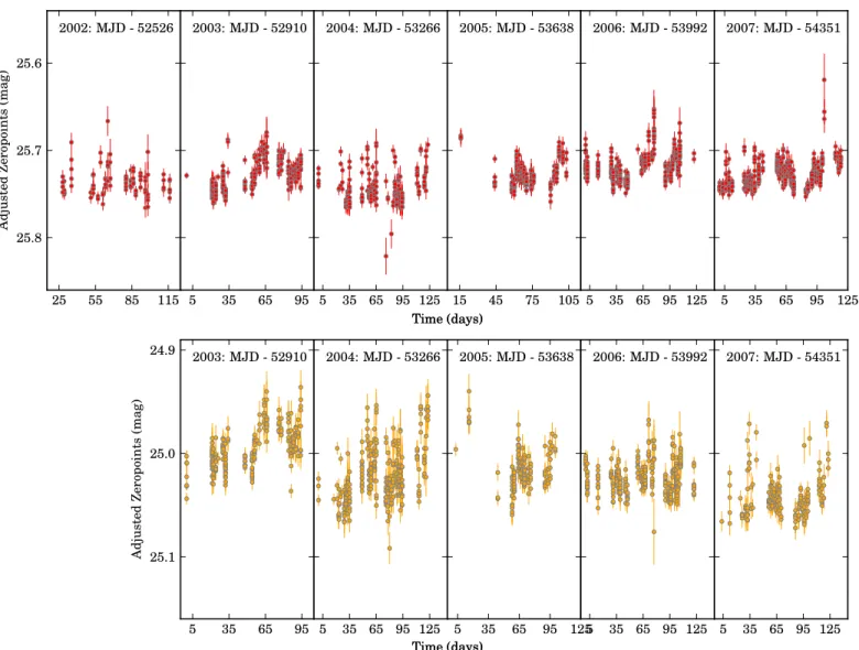
distribution of the reference catalog stars is shown in Figure6. These reference catalogs were used to determine zero points for all science images. To examine the temporal stability of the zero points, we adjusted them for differences in aperture correction, airmass, and exposure time, but not nightly variations in transparency or variation between different
31
amplifiers. The adjusted zero points of all available amplifiers were averaged together to construct the average adjusted zero point for a given image. In Figure7, we plot this quantity as a function of the time since the start of the each year’s observing season: the conditions at the Blanco remained very stable over
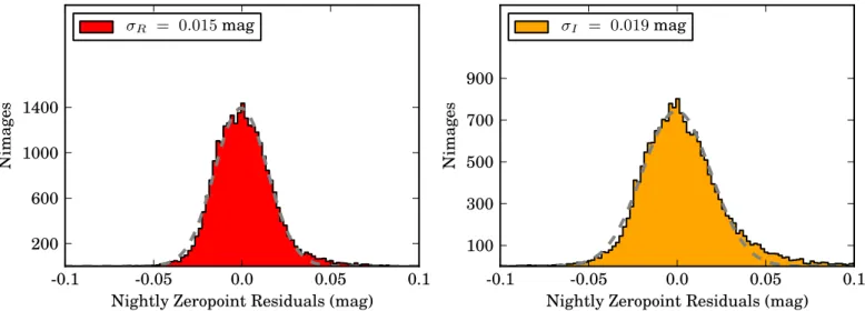
the entire duration of the survey. We also constructed the nightly average zero point, and the histogram of residuals to the nightly average zero point is plotted in Figure8. The residual scatter in the nightly zero point residuals is <2% in both
RandI.
Figure 5.Left:Extinction relation for CTIO Blanco system inRandIusing calibration data for three Landoltfields(L92, L95, and Ru149)imaged during the 2006 and 2007 observing seasons. The vertical axis is the difference between instrumental aperture magnitudes, and Landolt catalog magnitudes, corrected for exposure time and variation with LandoltR−Icolor. We exclude any data taken in non-photometric conditions. Wefind extinction law slopes of 0.104 mag airmass−1and 0.058 mag airmass−1inRandI,respectively. Right:Distribution of color terms, determined per-image, to LandoltR−Ifor the CTIO Blanco system inI(above)and
R(below), using calibration data from 2006 to 2007. Only images with at least 50 stars inRand at least 20 stars inIwere used in the analysis. As there are typically insufficient stars spanning the full color range in any single image, the weighted mean color term for all the images is computed(indicated by dashed vertical lines)and used for all further analysis. Wefind color terms ofcR-I = -0.0300.001
R L
4 m
( ) andcR-I =0.0220.001
I L
4 m
( ) .
3.6. Image Subtraction
Having established zero points for each science image, we used image subtraction to remove the background light of the host galaxies. Prior to subtraction, the PSF of each image was
first determined from field stars. We used the “High Order Transform Of PSF And Template Subtraction”(HOTPANTS)32
package to determine the convolution kernel between each image and template pair. For each pair, the image with the narrower PSF was convolved to match the image with the broader PSF. All N N( -1 2) possible pairs of image and reference templates from at least three observing seasons were used to create difference images for each object, following the algorithm of Barris et al.(2005). We used a version ofDoPHOT
(Schechter et al. 1993), modified to use the PSF and flux calibration of the image with the broader PSF, to measureflux in the difference image. Theflux calibration of the difference image was adjusted by the normalization of the convolution kernel. The position of the supernova was measured by taking the weighted mean of all detections with a S/N>5. The
derived positions are accurate to 0 02. The flux in each difference image was measured with the PSF centroidfixed to the position of the supernova. A representative example of our image subtractions is provided in Figure9.
As described in M07, the uncertainties in flux in our difference image are underestimated due to pixel–pixel covariance introduced during the re-sampling process. Rather than scale the noise in each image up by a constant factor of 1.2, as inM07, we determined a correction for each individual difference image using flux measurements across the frame. We convolved the PSF on a regular grid across the difference image, measured the standard deviation of the distribution of
flux sflux, and scaled each noise image by this factor. This
process effectively accounts for the small residual pixel–pixel covariance introduced by deprojecting each image onto a common astrometric grid, and by the PSF convolution.
Additionally, we constructed a light curve for each object using a single deep reference image, observed in photometric conditions with excellent seeing, to identify any potential problems introduced in processing the thousands of difference images produced by the NN2 process. We found excellent
Figure 7.Average zero points for imagesadjusted for differences in exposure time, aperture correction, and airmass over the full duration of the ESSENCE survey in
R(top)andI. In 2002, theIfilter(NOAO code c6005)was damaged and replaced. The zero point evolution is correlated in bothRandI, and the shorttimescale variations correspond to changes in weather conditions at CTIO, whereas the gradual drift in zero points is likely due to the increasing accumulation of dust in the optical system.
32
agreement between thefluxes measured in the single template and in the NN2 process, with the uncertainty in theflux being lower in the latter, as is expected by the use of multiple images to measure the galaxy template and sky background at each epoch.
4. SPECTROSCOPY
Our full sample consists of all SNIa for which we were able to obtain a positive spectroscopic identification. If possible, slits were aligned to obtain spectra of the host galaxies of the
SN candidates in order to obtain a more accurate redshift. The
first two years of spectroscopic data from ESSENCE were presented by Matheson et al.(2005), whileM07 detailed our selection criteria and classification algorithms. The spectro-scopic observations for the objects included in M07 were presented by Foley et al. (2009). The six-year spectroscopic sample from the ESSENCE survey is presented in this work, together with a summary of the spectroscopic observations, data reduction, and the process of candidate classification and redshift determination.
Figure 8.Histograms of the residuals ofR(left)andI(right)zero points to the average nightly zero point, adjusted for differences in exposure time, airmass,and the aperture correction. The measured scatter in the nightly zero point residuals is<2% in both passbands, consistent with the standard deviations derived from afit to a Gaussian distribution(dashed gray lines), and very comparable to the values found inM07, illustrating that zero points are very consistent fromfield tofield.
Figure 9.Representative difference imaging“postage stamps”inR(top)andI(bottom)forx025, a SNIa atz=0.35 near the median redshift of the survey. In this instance,HOTPANTShas convolved the PSF of the reference(left)to match the science image(middle). The reference is subtracted to produce the difference image
4.1. Selection Criteria for Candidates
As discussed in Section 2, over the sixyears of survey operation, ESSENCE detected thousands of objects exhibiting variability over multiple epochs, at a significance of S/N>5. Given the limited spectroscopic resources for followup, it was impossible to obtain spectra of all candidates. We employed various selection criteria to narrow the list of candidates from the imaging search to the subset with the most promise of being SNIa. Thefirst set of these selection criteria was implemented as software cuts in our search pipeline. We required the following.
1. Candidates detected in differences images have the same PSF as stellar objects in the source image that was convolved byHOTPANTS.
2. Candidates exhibit no significant negativeflux(<30% of the total number of pixels within an aperture of radius 1.5×FWHM around the detection) to select against difference image artifacts, such as dipoles resulting from slight image misalignment.
3. Candidates did not exhibit significant variability in ESSENCE data from previous yearsto reject variable stars and active galactic nuclei (AGNs).
4. Candidates in the difference image are not within 1 pixel (0 27) of objects in the template image, as these are frequently AGNs and spectra of such candidates suffer from excessive host galaxy contamination, making classification very uncertain.
5. Candidates exhibit at least two coincident detections with S/N>5, in at least two passbands or within afive-night window in a single passband, to reject moving objects within the solar system.
6. Detector and image reduction artifacts were excluded by visual inspection.
To select SNIa from the resulting list of candidates, wefit preliminary light curves using aBVtemplate of a normal SNIa (Dm15=1.1mag)constructed from well sampled low-zSNIa.
This template is a good match to SNIa observed in RI at
z∼0.4, typical for the ESSENCE survey. Usingc2
minimiza-tion, we determined the time ofBmaximum, theRImagnitudes at maximum, and the light curve stretch, s. These factors allowed us to determine an approximate photometric redshift for the object, which, along with theR−Icolorand rise-time information where available, was used to select likely SNIa.
An additional level of selection cuts was imposed by the observers on site. Observers tended to favor candidates thought to be in elliptical or low surface brightness hosts, as the former are reliably SNIa, while the latter aid in extraction of a clean spectrum. As the various facilities and instruments have different capabilities, and reach different depths, our faintest objects were preferentially observed at larger aperture facilities. We obtained spectroscopic followup using a range of facilities including the Blue Channel spectrograph on the MMT (Schmidt et al. 1989); IMACS on Baade(Dressler2004) and LDSS2(Allington-Smith et al.1994)and LDSS333on Clay at the Las Campanas Observatory; GMOS on Gemini North and South (Hook et al. 2003); FORS1 on the 8 m Very Large Telescope (VLT) (Appenzeller et al. 1998); and LRIS (Oke et al. 1995), ESI (Sheinis et al. 2002) and DEIMOS (Faber et al.2003)at the W. M. Keck Observatory.
Spectra were processed and extracted using standardIRAF
routines. Except for VLT data, all spectra were extracted using the optimal algorithm of Horne (1986). VLT spectra were extracted using a novel two-channel Richardson–Lucy restora-tion algorithm developed by Blondin et al.(2005)to minimize galaxy contamination in the target spectra. Spectra were wavelength calibrated using calibration lamp spectra (usually HeNeAr) fit with low-order polynomials, and were fl ux-calibrated using a suite of IRAF and IDL procedures, including the removal of telluric lines using the well-exposed continua of spectrophotometric standards.
To avoid relying on subjective assessments of noisy data, we employed the SuperNova Identification (SNID) algorithm (Blondin & Tonry 2007) to determine SN classifications objectively and reproducibly. SNID is based on the cross-correlation techniques of Tonry & Davis (1979). The input spectrum is compared to a large library of template spectra at zero redshift, including nearby SN of all types (SN Ia, Ib, Ic, II, and subtypes such as SN Ia-pec, SN 91 T, and SN 91bg; see Filippenko1997for a review of SN spectral classification), as well as other astrophysical sources such as luminous blue variables (LBVs) and other variable stars, galaxies, and AGNs. Where the redshift of the host galaxy is available, we forced SNID to look for correlations at that redshift(±0.02)to determine the SN classification. In general, the spectra of SN with z>0.5 have lower S/N, and thus ambiguities between types occurred mainly in that redshift range.
TheSNIDalgorithm has been presented by Matheson et al. (2005)and Foley et al.(2009), and we refer the reader to these publications for further details.
A list of all objects selected for spectroscopic follow up is provided in Table6. An analysis of the spectroscopic efficiency of the ESSENCE survey was presented in Foley et al.(2009). The redshift distribution of all ESSENCE SNIa is shown in Figure10.
Figure 10.Redshift distribution of spectroscopically identified SNIa from the ESSENCE survey. Candidates which have a high confidence of being of Type Ia(all objects whoseSNIDcorrelations with SNIa templates exceed 50%)are plotted in the shaded region. The histogram is shown for observing seasons spanning 2002–2003 (red), 2002–2005 (yellow), and 2002–2007
(blue), along withcumulativetotals, to illustrate the evolution of the redshift distribution over the course of the survey. Candidates for which we have less confidence have been classified “Ia?.” Several of these objects have well-measured redshifts from their host galaxies. These are shown in the open region.
33
ThefinalRIphotometry of 213 of the original 233 candidate SNIa objects presented in this paper is listed in Table7. Full light curves, including non-SNIa objects, and measurements of the baseline flux will be made available as machinereadable tables35along with this work. Photometry is presented in linear
flux units,f, in the Blanco natural system for each passband,T. Fluxes can be converted to calibrated magnitudes via:
f
= - +
mT 2.5 log10( T) 25. ( )5
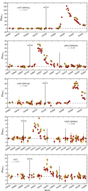
The system throughput curves and zero points required to derive magnitudes in our passbands from SED models using Equation (3) are provided in Appendix B. The ESSENCE SNIa and“Ia?”light curves are illustrated in Figure11.
5.1. Light Curve Shape and Color Distributions
Several different algorithms tofit SNIa optical photometry exist, including MLCS2k2(Jha et al.2007), BayeSN(Mandel et al. 2011), SALT2(Guy et al. 2007,2010), SiFTO(Conley et al. 2008), and Dm15 (Prieto et al. 2006). Each of these corrects for the shape and color relations, but they diverge when making two choices: the choice of how to train their spectral models and the choice of how to account for intrinsic and extrinsic color variations. This divergence results in a dichotomy between a physical model, where color variation is decomposed into an intrinsic variance and a reddening, attributed to extinction from dust (MLCS2k2 and BayeSN), versusan empirical model, where all color variation is directly correlated with luminosity (SALT2 and SiFTO). In the following subsection, we compare the color and shape parameter distributions derived using MLCS2k2 and SALT2 for the ESSENCE light curve sample presented in this work.
5.1.1. Light Curve Quality Cuts
While all the light curves arefit with both techniques, not all the fits are reliable, as several objects lack high-significance measurements of flux pre- or post-maximum, and these typically exhibit highc2 dof. Furthermore, objects in Table6
without determined redshifts are not fit.
Some selection cuts are common to all SNIa surveys, and are required to ensure that the light curvefit is well-constrained. These cuts are typically expressed in terms of the rest-frame
phase in rest-frame daysF =(TObs-TMax) (1+z). Kessler et al.(2009, hereafter K09)required at least one measurement withF <0.0. Guy et al. (2010, hereafter G10)36 employed a more flexible cut, only requiring a single measurement in the
Figure 11.Example ESSENCER(red)andI(orange)light curves, in units of linearflux, scaled such that aflux of unity corresponds to magnitude 25. Gaps between observing seasons have been removed, and the reported MJD is discontinuous at the locations of the vertical black lines. Thefirst of these lines is elongated and the year of the observing season is indicated to the left and right of it.
34
http://www.cbat.eps.harvard.edu/iauc/08200/08251.html
35
Available through FAS Research Computing at Harvard—http://
range of- < F < +8 5 days, and found that this provided a comparable constraint to the K09 cut. Similarly, WV07 required at least one observation with F+5 days for both MLCS2k2 andSALT, but also demanded that the observation had S/N>5, while requiring that the uncertainty on the fit time of maximum,sTMax,be<2days. TheWV07cut is effective
at ensuring that the time and the peakflux are well-constrained, and we adopt it here for ESSENCE SNIa. The compilation of 441 SNIa presented by Conley et al. (2011, hereafter C11) uses the weaker G10 cut on observations nearmaximum. In addition, G10do not impose any cut on S/N. However, these objects have observations in more passbands than ESSENCE, and the more conservative cut is appropriate.
When the cut on pre-maximum measurements is not applied, both the MLCS2k2 and SALT2 light curve shape parameters (Δandx1,respectively)exhibit a significantly increased scatter as a result of light curvefits being ill-constrained with only the post-maximum decline. Scolnic et al.(2014a)also reports that
x1shows a trend toward largervalues for z>0.4 if the pre-maximum data is excluded.G10did notfind such a trend with high S/N SNIa atz<0.4, illustrating how the effect of light curve quality cuts varies with median redshift, and therefore with survey.
WV07andK09also required that thefit statistic,c2 dof, be
<3for both light curvefitters.C11did not impose any quality-of-fit cut, as they felt that the reported uncertainties for low-z
photometry are frequently inaccurate, rendering such a cut misleading. They also suggested that several light curves contain the occasional outlying photometric observation that drivesc2 dof to artificially high values, despite having little to
no effect on the derived light curve shape and color parameters. C11also argues that anyc2-based cut has an asymmetric effect
with an SNIa sample, and therefore can potentially a introduce bias with redshift. This in turn could lead to systematic bias on
w. While there is merit in this argument, upon visual inspection of our light curve fits, we concluded that thec2 dofstatistic
did accurately represent the quality of thefit, and that this cut was well motivated. In future work, we will use Monte Carlo simulations to assess any biases in cosmological inference that result from this cut.
Another common cut is on the minimum number of degrees-of-freedom. Both WV07and K09requireNmin dof5.C11
do not explicitly state such a requirement, but the compilation they presented nevertheless satisfies that requirement. We adoptNmin dof5for MLCS2k2; however, we found that this
cut had the consequence of biasing us toward intrinsically brighter objects. WV07 also required one observation with
F +9 days for MLCS2k2. This cut was intended to ensure that the decline post-maximum is well sampled. As MLCS2k2 also imposes its own cut by requiring observations with S/ N>5, this cut is considerably more stringent than was intended. This requirement causes a total of 44 SNIa and
“Ia?”objects to fail the selection cuts—by far the single largest cut on our MLCS2k2 fits. In addition to eliminating observations of faint sources, or sources at high-z with extremely wellsampled declines, the S/N cut imposed by MLCS2k2 causes several light curves fits to fail the selection cuts as a result of an insufficient observations, given the requirement ofNmin dof 5 in the MLCS2k2fit.
By contrast, WV07 only required one observation post-B -band maximum forSALT, and only three objects in our sample do not meet this cut. We believe that this demonstrates that
MLCS2k2 is being needlessly conservative by requiring that all observations have S/N>5. However, the intent of the cut on the number of observations post-maximum is to ensure that the lightcurve extinction or color is well-constrained, and the location of the peak is bounded. We are wary of the relatively weak effect of the post-maximum cut on our SALT2 light curve fits, and require a stricter Nmin dof8 for that fitter.
With the ESSENCE four-day cadence, this effectively ensures that there are at least four measurements of the observer frame
R−I color. As a result, the number of objects that fail the Nmin dof cut for MLCS2k2 and SALT2 are similar, and some
of the most egregious outliers inx1and care eliminated. Based on the results inG10,C11imposed a restriction on the SALT2 color parameter, and required-0.25< <c 0.25mag. WV07did not explicitly impose an equivalent cut on AVfor
MLCS2k2. Several groups have used multi-color photometry of highly extinguished low-z SNIa to demonstrate that the extinction law in the host galaxies of these objects appears to follow the O’Donnell(1994)extinction law with a significantly lowerRV than the Milky Way(Hicken et al. 2009a; Folatelli
et al.2010; Mandel et al.2011).
Additionally, Scolnic et al. (2014b)employs a requirement that- <3 x1<3 for the Pan-STARRS1 SNIa sample. Both
these cuts are well motivated as there are few SNIa in the SALT2 training sample outside these ranges, and the fits are likely to be ill-conditioned there.WV07adopted a requirement of -0.4D 1.7. All objects in our ESSENCE SNIa sample that fail this requirementalso fail other selection cuts. A summary of the number of light curves that fail each cut for both MLCS2k2 and SALT2 is provided in Table2.
5.1.2. MLCS2k2 Light Curve Analysis
We employ“v007”of MLCS2k2 with the“tweaked-slowz” vectors. These vectors, and the corresponding matrix of model uncertainties (denoted S), are trained using the low-z
Hubble-Table 2
Effect of Light Curve Quality Cuts on the ESSENCE Sample
Cut MLCS2k2 SALT2
Notes. The number of SNIa and “Ia?” objects that are removed by each selection criterion. Each cut is imposed independently. Many objects fail multiple cuts.
a
We requireNmin dof8for SALT2, rather than the weaker cut of 5 for
MLCS2k2, as the last phase cut is very ineffective with SALT2 when our wellsampled NN2 light curves arefit influx space.
b
While atfirst glance it appears that more objects fail the cut on pre-maximum imaging with SALT2 than with MLCS2k2, this is not the case on closer inspection. MLCS2k2 merely fails catastrophically for objects without pre-maximum imaging, and consequently does not reportTMaxat all.
c
flow sample in Jha et al.(2007;hence“slowz”)and“tweaked” with small magnitude offsets(typically<0.005mag)to match the color–extinction distribution zero point, and extended to
−20days prior to B-band maximum. We follow WV07 in using the “glosz”prior on extinction, and assume RV =3.1.
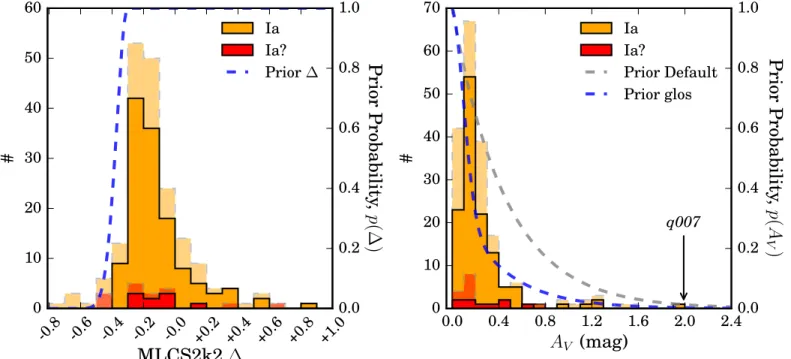
The MLCS2k2 light curve shape, Δ, and extinction, AV,
distributions for ESSENCE SNIa and“Ia?”objects are shown in Figure12. The MLCS2k2 light curve fit parameters for the ESSENCE sample are provided in Table 3. Additionally, we have indicated if the objects pass the light curve quality cuts used by WV07 for the four-year sample. From our spectro-scopically confirmed SNIa sample, 126 objects pass these cuts and are useful for cosmological inference. This doubles the 4year ESSENCE sample of 60 SNIa.
Objects withD >1.0are underluminous relative to normal SNIa, and are more rare. Consequently, we are extremely unlikely tofind any at the redshifts probed by the ESSENCE survey. Objects that appear to be extremely overluminous(very negative values of Δ) relative to the training sample of Jha et al. (2007) typically have little or no high-significance flux measurements pre-maximum, but have well-measured declines
post-maximum. Without a good constraint on the peak and time of maximum, light curve fitters typically explore unphysical regions of parameter space. The c2 dof of these
light curve fits is often relatively high (>3) and all fail the quality cuts of WV07, either owing to a high c2 dof or
because of insufficient observations pre-maximum.
TheAVdistribution for ESSENCE SNIa is consistent with
the “glos” model discussed employed by WV07. The distribution is significantly narrower than the MLCS2k2
“default” distribution, derived from nearby SNIa, as we are unlikely to find highly extinguished and therefore faint objectsat high-z. As MLCS2k2 is a magnitude based fitter, it rejects measurements with S/N< 5. Most of the objects that fail the selection cuts in the right panel of Figure 12 are extremely faint or at high-z.
Note that Figure12shows the distribution for all recovered
fits, and several of these objects do not have light curvefits that meet the quality cuts of WV07. Quality cuts are imposed to select spectroscopically confirmed SNIa, with several high S/ N measurements over rest-frame phase-5F20days, to ensure that the derived distance moduli are unbiased, whereas
Figure 12.Light curve shape,Δ(left panel), and extinction,AV(right panel), distributions estimated by MLCS2k2 for ESSENCE SNIa(orange)and“Ia?”(red) objects. Objects that pass the selection cuts(excepting the cuts on the parameter being plotted itself)imposed inWV07are indicated in the solid regions, while objects that fail are shown in the light regions bounded by dashed lines. The MLCS2k2 priors employed in the light curvefitting are shown as dashed blue lines. The“default” prior is the extinction distribution derived from low-zSNIa during the training procedure.
Table 3
MLCS2k2 Light Curve Fit Parameters for ESSENCE SNIa and“Ia?”Objects
ID μa s
m TmaxB sTmax FFirst b
FLast Δ sD AVc sAV Q
d
e108 42.370 0.140 52979.48 0.59 −11.768 9.954 −0.338 0.111 0.097 0.102 T k425 41.207 0.254 53335.19 0.43 −9.535 19.618 −0.087 0.177 0.310 0.236 T q002 41.212 0.359 54002.83 0.75 −6.340 15.192 0.594 0.279 0.549 0.369 T x080 42.006 0.440 54384.94 1.54 −4.178 17.699 0.132 0.343 0.315 0.276 T
Notes. a
MLCS2k2 reports distance moduli with aH0=65km s−1Mpc−1. bF
First Lastis the rest-frame phase of thefirst and last observation, respectively, and is dependent on theBbandtime of maximum,TmaxB .
c
We use the Galactic reddening law of O’Donnell(1994), withRVfixed to 3.1 to model the extinction in the host galaxy of the supernova. d
derived light curve shape and extinction are generally less susceptible to poor phase coverage.
5.1.3. SALT2 Light Curve Analysis
Additionally, we employ version 2.2.0b of SALT2 released together with G10. SALT2 is a flux-basedfitter and employs measurements of the baseline flux to restrict the search range forfitted parameters. However, only data within the rest-frame phase range -15< F < 45 days are used in the c2
minimization. Measurements in observer frame filters that map to the rest-frame wavelength range3000<l<7000 Å are used in the fit. Model and Kcorrection uncertainties are propagated into the error matrix, and an additional Uband
calibration uncertainty of 0.1 mag is added in quadrature for low-zNUV data.
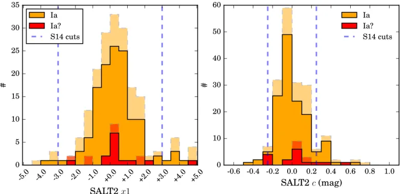
The SALT2 light curve shape,x1, and color,c, distributions for ESSENCE SNIa and“Ia?”objects are shown in Figure13. The SALT2 light curve fit parameters for the ESSENCE sample are provided in Table 4. Additionally, we have indicated whether the objects pass a combination of the light curve quality cuts used byWV07for the four-year sample, as well as shape and color cuts employed by Conley et al.(2011) and Scolnic et al.(2014b).
Objects withx1< -3.0andx1>3.0are poorly represented
in the SALT2 training sample. Fits with these values often have unconstrained rises or peaks, and provide unreliable distance estimates.
Figure 13.Light curve shape,x1(left panel), and color,c(right panel), distributions estimated by SALT2 for ESSENCE SNIa(orange)and“Ia?”(red)objects.
Objects that pass the originalSALTselection cuts(except the cuts on the parameter being plotted itself)imposed byWV07are indicated in the solid regions, while objects that fail are shown in the light regions bounded by dashed lines. Only theWV07cuts relating to the sampling andc2 dofof thefit are used here. Based on a visual inspection of all the light curvefits, we required that thefits used at least eightepochs, rather than the weaker cut of at leastfiveepochs employed forSALT
inWV07. We employ the same cuts as Conley et al.(2011)and Scolnic et al.(2014a)oncandx1,respectively.
Table 4
SALT2 Light Curve Fit Parameters for ESSENCE SNIa and“Ia?”Objects
ID mBa smB mV smV T B
max
b
sTmax x1 sx1 c
c
sc Cov ,(c x1)
d
Qe
b010 23.4583 0.0666 23.5138 0.0937 52593.2578 0.8841 0.9105 0.7618 −0.0781 0.1012 0.0248 T g050 23.2239 0.0702 23.4278 0.1084 53302.2280 0.5811 −0.2400 0.5682 −0.2226 0.1069 0.0153 T h323 23.4921 0.0594 23.3174 0.0873 53329.8365 0.6337 0.6074 0.5493 0.1485 0.0930 0.0094 F n322 24.3561 0.0919 24.4587 0.2019 53707.8798 1.4726 0.1779 1.0967 −0.1237 0.1342 0.0518 T
Notes. a
SALT2 does not directly report distance estimates. The distance modulus is determined using a globalfit for all SNIa together with other cosmological parameters. b
While the SALT2 shape estimates are strongly affected by measurements pre-maximum, it uses significantly more low S/N measurements on the decline, as well as measurements for faint and/or high-zobjects. Consequently, the cut on number of measurements post-maximum has very little impact. We instead require a total of eightobservations be used in thefit to ensure that the measured parameters are reliable.
c
We use the updated SALT2 color law described by Guy et al.(2010). This differs significantly from the O’Donnell(1994)extinction law in the near-UV. d
Covariances between all thefit parameters—Cov(mB,x1), Cov(mB,c), and Cov(x1,c)—are calculated, and these values will be included in the machine readable tables
provided with this work. e