The role of urban green infrastructure in mitigating land
surface temperature in Bobo-Dioulasso, Burkina Faso
Ne´stor Di Leo1•Francisco J. Escobedo2•
Marielle Dubbeling3
Received: 13 November 2014 / Accepted: 5 March 2015 / Published online: 15 March 2015
Springer Science+Business Media Dordrecht 2015
Abstract Green infrastructure in developed countries has been used as a climate change adaptation strategy to lower increased temperatures in cities. But, the use of green in-frastructure to provide ecosystem services and increase resilience is largely overlooked in climate change and urban policies in the developing world. This study analyzed the role of urbanization and green infrastructure on urban surface temperatures in Bobo-Dioulasso, Burkina Faso, in sub-Saharan Africa. We use available geospatial data and techniques to spatially and temporally explore urbanization and land surface temperatures (LSTs) over 20 years. The effect of specific green infrastructure areas in the city on LSTs was also analyzed. Results show increased urbanization rates and increased temperature trends across time and space. But, LST in green infrastructure areas was indeed lower than adjacent impervious, urbanized areas. Seasonal phenological differences due to rainfall patterns, available planting space, and site limitations should be accounted for to maximize temperature reduction benefits. We discuss an approach on how study findings and urban and peri-urban agriculture and forestry are being used for policy uptake and formulation in the field of climate change, food security, and urbanization by the municipal government in this city in Burkina Faso.
1 Center for Territorial Studies, Faculty of Agricultural Sciences, National University of Rosario,
Parque Villarino, C. C. 14, S2125ZAA Zavalla, Santa Fe, Argentina
2
School of Forest Resources and Conservation, University of Florida-IFAS, 361 Newins-Ziegler Hall, PO Box 110410, Gainesville, FL 32611, USA
3
RUAF Foundation-International Network of Resource Centres on Urban Agriculture and Food Security, Kastanjelaan 5, 3833 AN Leusden, The Netherlands
Keywords Urban agricultureUrban forestryUrban ecosystem servicesUrban climate change policiesUrban heat islandAfrica
1 Introduction
Economic development and investment by developing countries to address the negative impacts of urbanization and climate change are generally focused on urban infrastructure improvements and engineered risk reduction (Tosam and Mbih2014; UN-Habitat2014). The use of open and vegetated spaces in cities to provide ecosystem services and increased resilience is also largely overlooked in policies and studies (Cilliers et al.2012; Escobedo et al.2011). This use of soils and vegetation to mitigate urban environmental problems is often referred to as ‘‘Green Infrastructure’’ which can consist of various activities such as urban and peri-urban agriculture and forestry (UPAF) or nonproductive (ornamental) ac-tivities and green land covers at various scales (e.g., trees, parks, gardens, private, and public open spaces; Cilliers et al.2012; Norton et al.2015). Although frequently used to mitigate increased temperatures and pollution in developed countries, its use for envi-ronmental quality and food security improvement in developing countries such as those of sub-Saharan Africa has been little studied (Escobedo et al. 2011; Cilliers et al. 2012; Scha¨ffler and Swilling2013; UN-Habitat2014).
Below, we review the literature on the role of green infrastructure in mitigating urban surface temperatures with an emphasis on medium-sized sub-Saharan African cities. First, we discuss the role of urbanization on increased surface temperatures and the effects of these temperatures on human well-being. The literature on how urban vegetation mitigates these temperatures and the methods used to measure urban surface temperatures are then reviewed. Third, we present studies that spatially and temporally quantify urbanization and land surface temperatures (LSTs) using available satellite imagery and remote sensing techniques to measure the effect of specific green infrastructure areas on surface tem-peratures. Finally, we present an approach for analyzing the role of green infrastructure in mitigating surface temperature and its integration into urbanization and climate change policies in a city in sub-Saharan Africa as well as other parts of the developing world.
1.1 Urbanization and green infrastructure: effects on surface temperature
et al. 2012; Landsberg1981). Referred to as the urban heat island (UHI) effect, higher urban temperatures are caused by anthropogenic heat released from vehicles, power plants, air conditioners, and other heat sources, and heat stored and re-radiated by massive and complex urban structures (Rosenfeld et al. 1998). The UHI effect can be reduced using building and urban design strategies such as the use of highly reflective building materials and roofs as well as appropriate building designs and vegetation management and place-ment (Rosenfeld et al.1998).
Conversely, urban and peri-urban vegetation modify surface and atmospheric tem-peratures in cities due to evapo-transpiration, shading, and albedo effects (Bowler et al.
2010; Jonsson2004; Cavan et al.2014; Norton et al.2015). Increasing or conserving green infrastructure in cities has thus been proposed as a strategy to regulate temperatures (Oliveira et al.2011; Cavan et al.2014; Norton et al.2015). These vegetated surfaces, such as green walls and roofs, gardens, green spaces, lawns, and trees, can also capture solar radiation to different extents and ultimately reduce the UHI (Bowler et al.2010; Brown and Gillespie1995).
For example, Amiri et al. (2009) and Shashua-Bar et al. (2009) found that urban vegetation can lower temperatures in hot, arid cities in Iran and Israel, respectively. Oli-veira et al. (2011) and Lin and Lin (2010) also looked that the cooling effects of vegetated, urban spaces in Portugal and subtropical China, respectively. Cavan et al. (2014) studied the role of different urban morphologies in regulating LSTs in Addis Adaba, Ethiopia, and Dar es Salaam, Tanzania, and found that residential areas with large green spaces in both these cities had lower surface temperatures. Conway et al. (2004), Goldreich (1992), and Jonsson (2004) also documented such climate effects in Addis Adaba and Johannesburg as well as urban vegetation effects on climate in Botswana, respectively. However, these are among the very few of the studies implemented in sub-Saharan Africa on this topic in the available English language literature.
Recently, measurement of LST has been proposed as an alternative to measuring air temperature (Cheng et al.2008; Cavan et al.2014). Airborne or satellite sensing techniques are particularly useful for remote measurements (Streutker 2003), and now LST mea-surements have become common in urban climatology (Voogt and Oke 2003; Li et al.
2013).
Remote sensing data have been utilized for local-scale studies (Weng2001; Wang et al.
2004; Cao et al. 2010) and are based on the relationship between LST and vegetation abundance (e.g., Gallo and Owen1998a,b; Weng2001; Weng et al.2004). Lin and Lin (2010) used Landsat TM data to analyze the temperature effects of urban parks on adjacent areas in China. Amiri et al. (2009), Cao et al. (2010,2012), Cheng et al. (2008), and Yuan and Bauer (2007) also analyzed the effects of vegetated landscapes on urban temperatures using various types of satellite data.
1.2 Objectives
measured by normalized difference vegetation index (NDVI) is related to cooler LSTs. We then discuss how our findings and green infrastructure can be incorporated into existing Bobo-Dioulasso’s urban planning policies to regulate temperatures and adapt to climate change.
2 Methods
2.1 Study area
Bobo-Dioulasso is Burkina Faso’s second most populous city and is located at 111100000N and 41700000W and a mean altitude of 445 m (Fig.1). The urban area is about 136,78 km2 and has 435,543 inhabitants according to the 2006 census (INSD2007), with a growth rate of 7.23 % and a density of 3,184 inhabitants/km2. According to the Ko¨ppen-Geiger system, it has a tropical savannah (Aw) climate (Peel et al.2007). The average monthly maximum temperature ranges from 29.4 to 36.9C, average annual minimum temperature is 20.6, and it receives 1050 mm of precipitation per year (www.Climate-Data.org, 2014; www. Wather2Travel.com, 2014; ‘‘Appendix’’).
Between 1926 and 1929, the French colonial government constructed the city’s layout using a grid pattern with avenues and streets, intersected by diagonals radiating from a center, with square urban lots between them. This laid the framework for the modern city center and its land uses (Fouchard2003). New industry arrived in the city during the 1980 and 1990s. Since 2000, the city of Bobo-Dioulasso has experienced rapid urbanization, population increases, and economic vitality (N. Gahi, Municipalite´ de Bobo-Dioulasso, Personal Communication, 2013).
2.2 Remote sensing data and software
Our Bobo-Dioulasso study area was outlined using a parallelogram-shaped polygon to facilitate multi-temporal comparisons of LULC and LST conditions. The northwest vertex for the study area was 1117012.000N; 0420033.400W. A total of 24 images with good a priori radiometric conditions were downloaded from the USGS server (earthexplorer.us-gs.gov; Table1). Eight images were affected by cloudiness or haze and were discarded. In total, the analysis was based on 16 processed images from three different sensors. All three optical-band sensors had a spatial resolution of 30 m, and the thermal infrared band had a spatial resolution of 120 m for Landsat 5 TM, 60 m for Landsat 7 ETM?(band 6 in both sensors), and 100 m for Landsat 8 OLI-TIRS images (band 10). October 2012 Google Earth images and areas of potential interest to municipal authorities were used to visually interpret specific urban morphologies and identify green infrastructures.
Noise reduction corrections and co-registration between multi-temporal images were performed using Ilwis 3.8 software (ILWIS2011). Landsat TM and ETM?sensors have only one thermal infrared band (10.44–12.42 mm), which precludes the use of general
Table 1 US Geological Survey
20/04/2000a Landsat 7 ETM? 197 52
15/05/2000a Landsat 7 ETM? 196 52
11/09/2000a Landsat 7 ETM? 197 52
02/02/2001a Landsat 7 ETM? 197 52
01/09/2002a Landsat 7 ETM? 197 52
8/2/2003 Landsat 7 ETM? 197 52
08/05/2003a Landsat 7 ETM? 196 52
22/10/2006 Landsat 5 TM 197 52
14/06/2011a Landsat 5 TM 197 52
29/10/2011 Landsat 5 TM 196 52
3/6/2013 Landsat 8 OLI-TIRS 197 52
12/6/2013 Landsat 8 OLI-TIRS 196 52
9/10/2013 Landsat 8 OLI-TIRS 197 52
25/10/2013 Landsat 8 OLI-TIRS 197 52
split-window correction algorithm possible, thus only band 10 was corrected for the Landsat 8 OLI-TIRS sensor and was used jointly with Landsat 5/7 TM/ETM?band 6.
We then used a non-supervised classifications of the September 11, 1991, TM and October 25, 2013, OLI-TIRS images to analyze changes in Bobo-Dioulasso. To determine differences in LSTs between areas of highly built impervious surface covers and green infrastructure areas, we performed the four steps detailed in the following Sect.2.3. Re-sults were then used to analyze relationships between LST and NDVI using spatial re-gressions between each LST image and the NDVI image as we will describe in Sect.2.4.
2.3 Derivation of brightness temperature
The signals received by the thermal sensors (TM/ETM?/OLI-TIRS) were converted to at-sensor radiance using Eq. (1):
Lk¼GkDNkþBk ð1Þ
whereLkis spectral radiance of thermal band in W/m2ster mm;Gk(gain) is the slope of the radiance/DN conversion function; DNkthe digital number of a given pixel from an L1G product; and Bk (bias) is the intercept of the radiance/DN conversion function (Landsat Project Science Office2002). Gain and bias values are from Chander et al. (2009) for TM and ETM? images and in the header files of OLI-TIRS images. Subsequently, radiance values from the TM/ETM?/OLI-TIRS thermal band were transformed to radiant surface temperature (i.e., top-of-atmosphere brightness temperature) using thermal calibration constants supplied by the Landsat Project Science Office (2002) in Eq. (2):
TB¼K2=ðlnðK1=Lkðþ1ÞÞ ð2Þ
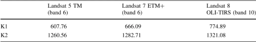
whereTBis the effective at-satellite brightness temperature in Kelvin; K1 (watts/(meter squared9ster9lm)) and K2 (Kelvin) are calibration constants obtained from the USGS website (TM/ETM?) and from the header file of Landsat 8 OLI-TIRS images (Table2); and Lkis the spectral radiance in watts/(m2sterlm).
2.4 Using normalized difference vegetation index (NDVI) to estimate land surface emissivity (LSE)
The LST estimation using passive thermal remote sensing depends on accurate emissivity specification (Becker and Li1990; Valor and Caselles1996); therefore, we used the NDVI [Eq. (3); Elhag2014] to determine LSE.
NDVI¼NIRR
NIRþR ð3Þ
where NIR is the spectral reflectance corresponding to the near-infrared band of TM/ ETM?(band 4) or OLI-TIRS (band 5) andRthe spectral reflectance of the red band of the
Table 2 Calibration constants used for effective at-satellite brightness temperature (TB) retrieval in Eq. (2)
two sensors (band 3 and band 4, respectively). The vegetation cover method developed by Valor and Caselles (1996) is based on the relationship between emissivity in the thermal infrared and the NDVI and shows that LSE varies with the proportion of vegetation/bare soil or impervious surfaces within each pixel.
As the reflective bands of Landsat sensors have a spatial resolution of 30 m, but TIR bands have a coarser spatial resolution (120 m for TM band 6, and 100 for OLI-TIR band 10), we assumed that all the pixels were composed of a matrix of bare soil, impervious, and vegetation surfaces, and we calculated emissivity according to Eq. (4).
LSE¼evPvþesð1PvÞ þde ð4Þ
whereev andesare vegetation and soil emissivity, respectively, and Pvis the vegetation
proportion obtained according to Carlson and Ripley (1997), Eq. (5):
Pv¼
NDVINDVImin
NDVImaxNDVImin
2
ð5Þ
Values for NDVImaxand NDVIminwere obtained from each image’s histogram. The term
dein Eq. (4) includes the effect of the geometrical distribution of the natural surfaces and the internal reflections. For plain surfaces, this term is negligible, and for heterogeneous and rough surfaces it can reach a value of 2 % (Sobrino et al. 2004). Following the methodology, we used a soil and vegetation emissivity of 0.97 and 0.99, respectively, and Eq. (6) provides the equation used for estimating LSE.
LSE¼0:004Pvþ0:986 ð6Þ
We also used NDVI to estimate the land surface emissivity (LSE) Eqs. (3–6) by testing it as predictor of LST variability within the study area. The ordinary least squares ‘‘regress’’ module in Ilwis v3.8 software was used for defining the NDVI images as independent and the LST images as dependent variable for the Landsat 8 OLI-TIRS acquired on 2013. Statistical differences were tested with the Wilcoxon sign rank test with the subroutine wilcox.test in the R version 3.0.1 statistical software.
2.5 Retrieval of LST
The emissivity corrected LST was computed with Eq. (7) (Artis and Carnahan1982).
LST¼ TB
1þðkTB=qÞln LSE ð7Þ
wherekis the wavelength of emitted radiance or the peak response and the average of the limiting wavelengths (k=11.5lm), q=hxc/r(1.438910-2m K),r is Boltzmann constant (1.38910-23 J/K),h is Planck’s constant (6.626910-34 J s), and c is light velocity (2.9989108 m/s). Since the surface radiant temperature was in Kelvin, the radiant temperature was converted using absolute zero (approximately 273.15C) (Xu and Chen2004) in Eq. (8).
LST¼ TB
1þðkTB=qÞln LSE273:15 ð8Þ
reflect the distribution of the surface temperature fields (Chen et al. 2002). Since water vapor varies temporally due to inter-annual variability and atmospheric conditions, we focused on the spatial patterns of LST across the study area for the image acquisition dates. Specifically, LST intensity was measured as the difference between temperature inside highly urbanized land uses and areas of urban and peri-urban green infrastructure (Voogt and Oke 2003). In doing so, spatial and temporal LST effects can be measured across thermal images (Li et al. 2013). We accounted for season differences by grouping ac-quisition dates into ‘‘wet and cool’’ (May–September) and ‘‘dry and hot’’ (October– April) seasons (see ‘‘Appendix’’).
2.6 LST spatial heterogeneity
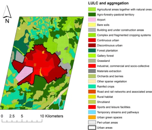
We used 2002 LULC data from the Geographic Institute of Burkina Faso (IGB 2002; Fig.2). Using these data and image interpretation of the degree of human intervention, twenty-two different LULC classes were initially aggregated into one urban and one peri-urban LULC class that were the basis for the LST and NDVI analyses (Fig.2). To char-acterize the impact of green infrastructure areas within Bobo-Dioulasso, we digitized specific UPAF areas using Google Earth as well as cartographic information and input provided by the city government (Fig.3a). Eight specific areas identified as UPAF were mapped in the study area. Each area consists of polygons or ‘‘islands’’ that varied from 4.2
to 10.4 hectares in size. Site-specific LSTs were calculated for images from 08/02/2003 to 25/10/2013 to test for differences between LSTs in highly built urban areas and specific green infrastructure areas (Fig.3b). Both 1991 images were excluded from this analysis since UPAF activities had not yet been established at this time.
3 Results and discussion
3.1 Urbanization patterns
Temporal analysis shows the magnitude and pattern of urbanization from 1991 to 2013. Denser urban land uses doubled by almost 7800 hectares. A comparison between the white or gray urban zones in the 1991 TM and 2013 OLI-TIRS images revealed a noticeable
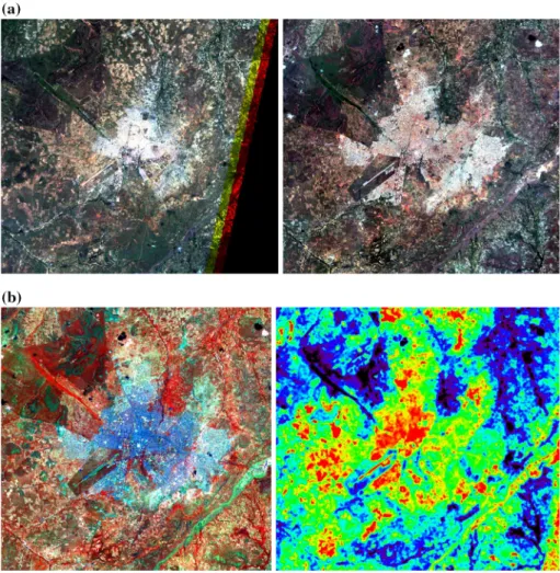
Fig. 3 a Bobo-Dioulasso using a natural false color composition (RGB 321 and RGB 432) Thematic
Mapper image dated 11/09/1991 (left) and an OLI-TIRS image acquired on 25/10/2013 (right) using the
same scale.bBobo-Dioulasso using Landsat 8 OLI-TIRS with reflective 564 bands (left;lightanddarker
bluesshowing urban areas,orangesandredsshowing vegetated areas) and thermal infrared band 10 (right;
expansion of urbanized areas and decreased green infrastructure areas (Fig.3a). The same contrast in LST between urban and peri-urban areas is visible in Fig.3b.
3.2 Land surface temperature differences
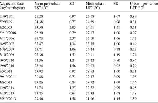
The LST of the highly urbanized areas was greater than peri-urban LULC within the study area (Table3; Figs.3b,4). Temporal differences in LST between urban and peri-urban areas increased over the analyses period by approximately 6 % per year (Table3; LST=0.0579x?0.5563; R2=0.29). The LST shows similar spatial distribution in urban areas in all images, but this pattern was not evident in peri-urban areas due to seasonal differences in the images (‘‘Appendix’’).
Mean differences in urban and peri-urban LSTs during the ‘‘wet and cool’’ and ‘‘dry hot’’ periods were 0.781 and 1.375C, respectively. We note that seven of the nine images from the wet and cool season were taken in the start of the growing season. So, pastures, crops, and natural vegetation in peri-urban areas are likely in their initial growth stages and might be revealing areas with bare soil. But, the number of available images was insufficient to test for differences between seasons due to variation in monthly mean temperature and rainfall as this is limited to 5 months, causing variations in the phenology of the peri-urban vegetation.
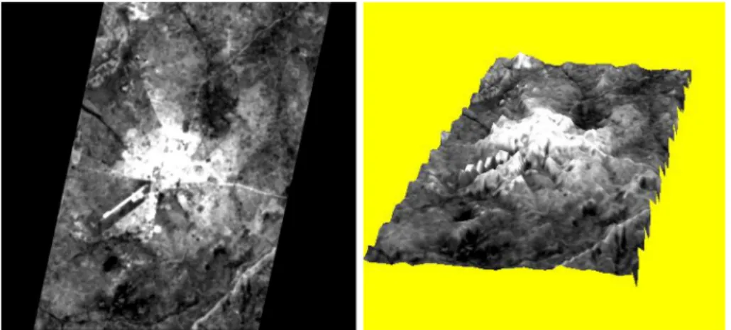
Very high LST was visible on arable lands (Fig.3b). For some images, LSTs in agri-cultural or pasture areas were characterized by low vegetation cover (i.e., seasonal phe-nology, temporal drought, harvests). These areas can warm rapidly during the morning hours, and low vegetation cover could also infer drier conditions and low latent heat transfer. Several green infrastructure islands such as city parks and recreational areas were visible inside the urban matrix (Figs.2,3). The LST influence on the UHI is particularly evident in the 09/10/2013 image (Fig.5) where increased LSTs are found in the city core
and these decrease as one moves toward the peri-urban and rural zones in the study area. Overall, these findings corroborate those from our literature review in Sect.1.2, but sea-sonal dynamics and vegetation phenology in the surrounding peri-urban areas are also affecting LST variability.
Fig. 4 Land surface temperature (LST) trends in Bobo-Dioulasso, Burkina Faso, for the dates of acquisition of the remotely sensed (RS) images
Fig. 5 Land surface temperature image (left) and three-dimensional model (right) for Bobo-Dioulasso,
Burkina Faso, acquired on 9/10/2013 (left). Increased temperatures are represented by lighter colored and
higher elevation pixels; conversely cooler temperatures are represented by darker colored and lower
3.3 Green infrastructure effects on land surface temperatures
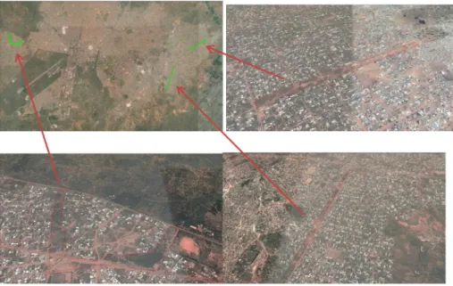
The LULC maps depicting zoned land uses with green infrastructure (Fig.5a) did not match well with the actual spatial characteristics observed in Google Earth. Thus, we limited our analyses on the role of specific green infrastructure areas on reducing LSTs to three specific islands (Fig.6; green infrastructure areas 5, 6, and 8). This lack of dis-cernable green infrastructure areas is probably because of irregular or non-designated land uses such as transportation corridors, non-zoned housing, and construction parcels.
The mean LST of these green infrastructure areas was lower compared with adjacent built-up LULCs across the study area (Table4). This despite the green infrastructure areas being linear and thus the green infrastructure signals were mixed with immediately ad-jacent urban built-up pixels. Only 55 pixels represented these areas due to the low spatial resolution from the remote sensor thermal bands (120 m for L4-5 TM. 60 m for L7 ETM?
and 100 m for the new Landsat 8 OLI-TIRS). Overall, we also found that mean LST over a 10 year period was consistently cooler (0.3C) in these green infrastructure areas than in adjacent built-up areas as shown in Table4. Green infrastructure areas in the 12/06/2013 image (Fig.7) show lower LST than adjacent urban areas. But again, the thermal images show the effect of climatic seasons and/or seasonal phenological differences on the green infrastructure’s vegetation.
Negative correlations between LST and vegetation activity and/or abundance (i.e., NDVI) support our hypothesis that the occurrence of vegetation can significantly reduce LSTs. Specifically, our LST-NDVI analysis also shows significant negative correlations (Table5) and explained variance reached 63 % for the best fit on the 09/10/2013 image. Ordinary least square regression analyses suggest that NDVI can better explain LST during the rainy season because of increased vegetation abundance.
Fig. 6 Google Earth image showing the 3greeninfrastructure areas that were analyzed for temperature
differences (upper left). Theupper right,lower left, andlower rightimages show the location ofgreen
Our results (R2 of 0.48–0.63) corroborate those of Hu and Jia (2010) who found that NDVI explained 61 % of LST variability. However, other characteristics affecting LST and UHI intensity also include urban morphology, location, and climatic zone. Yuan and Bauer (2007), for example, concluded that the relation between LST and percent imper-vious surface is more significant while NDVI importance is less strong and the role of vegetation varies with seasons.
Table 4 Mean, standard deviation (SD), and difference between land surface temperatures (LSTs) of green
infrastructure (GI) areas (n=3) in Bobo-Dioulasso for the dates of acquisition of remotely sensed images
Acquisition date
Fig. 7 Land surface temperature (LST) image acquired on 12/06/2013 (left) and a high resolution Google
Earth image of green infrastructure area 33 (right).Leftimage shows the more vegetated areas in the west
sector of green infrastructure and surroundings areas.Rightimage shows areas of bare soil near a primary
school in the east sector of green infrastructure. Thegreenpolygon in theleft imageshows lower LSTs in
the east sector of an area withgreeninfrastructure (green rectanglesin theright image) caused by high
3.4 Using green infrastructure to mitigate land surface temperatures
Our study characterized the spatial and temporal role of green infrastructure on LST for a medium-sized sub-Saharan African city. High spatial resolution Landsat series (120 m for L4-5 TM. 60 m for L7 ETM?, and 100 m for the new Landsat 8 OLI-TIRS) data can therefore be used for local multi-temporal thermal infrared studies. Available Landsat 8 OLI-TIRS images, coupled with in situ climatic and/or radiometric measurements, can ideally be used for future research and validating this study’s results. Additionally, in-corporating horizontal and vertical urban morphology typologies could improve results (Cavan et al.2014). Correlations between temperature and imperviousness indices or other transformations could also disaggregate mixed pixels with a greater degree of certainty.
The study’s quantification of LST differences between urbanized and green infrastructure areas corroborates findings from other global studies from Sect.1.2that indeed open and green space areas with pervious soils and vegetation cover have lower temperatures than adjacent impervious urban areas (Bowler et al.2010; Cavan et al.2014; Gallo and Owen
1998a,b; Lin and Lin2010; Norton et al.2015; Weng2001; Weng et al.2004). Given Bobo-Dioulasso’s climate and economic realities, these reduced LSTs provide an indicator of the ecosystem services being provided by green infrastructure (Cilliers et al.2012) and their value in improving human well-being (Scha¨ffler and Swilling 2013). Although not specifically quantified, these areas are also providing other regulation (e.g., carbon seques-tration, reduced stormwater runoff), provisioning (e.g., food and fuel from urban agriculture), and cultural (e.g., recreation) ecosystem services to urbanites (Cilliers et al.2012; Elhag
2014; Escobedo et al.2011; Scha¨ffler and Swilling2013; UN-Habitat2014)
We acknowledge the limitations of this study when using only sixteen images for a 20-year analysis. We also note the lack of available and detailed geospatial data for Bobo-Dioulasso. In particular, thermal remote sensing data using satellite sensors were not available at finer resolutions for this study. However, our approach using available geospatial data shows how LST increases from urbanization can be feasibly and technically documented. Our approach and findings also show the role of green infrastructure in mitigating LSTs and might be of interest to urban planners and authorities from the developing world interested in adapting to future climate change impacts (Bowler et al.2010; Tosam and Mbih2014). Further, with rapid advances in remote sensing technologies, soon new satellite thermal sensors with higher resolution, and thermal cameras mounted on unmanned aerial systems, will facilitate more detailed spatiotemporal analyses of UHIs and LST (Li et al.2013).
We do note that green infrastructure, particularly in a climate such as this study area, might require additional irrigation; thus, stormwater harvesting and recycling of graywater (i.e., ‘‘blue infrastructure’’) could be used to irrigate and maximize the cooling effects of green infras-tructure (UN-Habitat2014). Otherwise, given the lack of stormwater infrastructure and water
Table 5 Linear regression performed between land surface temperatures (LSTs) and normalized difference vegetation index (NDVI) for the Landsat 8 OLI-TIRS images acquired on 03/06/2013
Acquisition date (day/month/year)
Regression equation rcoefficient R2coefficient t-stat for r
orb
03/06/2013 LST=29.63–6.399NDVI -0.69 48.22 -570.95
12/06/2013 LST=34.67–8.219NDVI -0.75 55.45 -660.15
09/10/2013 LST=26,781–5.929NDVI -0.79 63.03 -772.60
25/10/2013 LST=33.49–9.609NDVI -0.73 52.64 -623.83
recycling technologies in resource limited communities, the use of xeric vegetation and in situ water conservation practices is recommended (Norton et al.2015; Tosam and Mbih2014).
4 Conclusions
This approach can be used to assess whether green infrastructure and UPAF activities lower temperatures in cities of the developing world. Such information will lead to a better under-standing how urban and green infrastructure planning and management reduce LSTs in sub-Saharan African cities (Bele et al.2014; UN-Habitat2014). In particular, our results are relevant to policy makers from cities in developing countries interested in the potential impacts of climate change and urbanization on human well-being (Tosam and Mbih2014). Our literature review demonstrates how higher LSTs in urban areas negatively affect public health, energy use, and environmental quality (Bowler et al.2010). Thus, promoting UPAF and other forms of green infrastructure can contribute to helping communities adapt to climate change. Indeed, local governments in the developing world are using UPAF activities for other co-benefits such as food security and flood mitigation (Cilliers et al.2012; Escobedo et al.2011; UN-Habitat2014). Additionally, research on the benefits of preservation of green infrastructure is highly relevant as municipalities in Africa, as elsewhere, regularly encourage infill developments and higher housing densities that lead to the reduction or loss of green spaces and gardens. Since this project was done in collaboration with local authorities, in 2014 preliminary findings from this study were used by the municipality of Bobo-Dioulasso to develop three policy guidelines on the management and use of green infrastructure that were adopted by the Environmental Commission. These three guidelines lay out the basis for: (1) the creation, composition, and functioning of a municipal committee that will be in charge of the future management of the greenways, (2) a new technical statute for the greenways, including a productive land use component, and (3) a management charter related to the urban greenways.
As such, science-based information can improve policy uptake and promotion of these three policies to the Municipal Council of Bobo-Dioulasso. Doing so will ensure that budgets are made available for their implementation. Approval will also require the municipality to allocate further funding for the management of existing and proposed green infrastructure, to strengthen the municipal department of the parks department (i.e., the main technical partner for green in-frastructure management), and to ensure the functioning of the proposed committee in charge of the greenways. We suggest that findings from this study and their incorporation into policies will ensure that longer-term municipal strategies can be put in place to support multifunctional development of the green infrastructure as part of the city’s climate change adaptation strategy.
Acknowledgments We thank Narcisse Gahi, Institute d’application et de vulgarisation en sciences- IAVS in Ouagadougou and Hamidou Baguian, Municipalite´ de Bobo-Dioulasso for support with data. This study was coordinated by the International Network of Resource Centres on Urban Agriculture and Food security (RUAF) and funded by UN-Habitat Cities, Climate Change Initiative, the UK Department for International Development (DFID), and the Netherlands Directorate-General for International Cooperation (DGIS) for the benefit of developing countries. However, views expressed and information are not necessarily those of, or endorsed by UN Habitat, DFID, DGIS, or the entities managing the delivery of the Climate and Devel-opment Knowledge Network, which can accept no responsibility or liability for such views, completeness, or accuracy of the information or for any reliance placed on them.
Appendix
References
Amiri, R., Wen, Q. H., Alimohammadi, A., & Alavipanah, S. K. (2009). Spatial-temporal dynamics of land surface temperature in relation to fractional vegetation cover and land use/cover in the Tabriz urban
area, Iran.Remote Sensing of Environment, 113(12), 2606–2617.
Artis, D. A., & Carnahan, W. H. (1982). Survey of emissivity variability in thermography of urban areas.
Remote Sensing of Environment, 12, 313–329.
Becker, F., & Li, Z. L. (1990). Temperature independent spectral indices in thermal infrared bands.Remote
Sensing of the Environment, 32, 17–33.
Bele, M. Y., Sonwa, D. J., & Tiani, A. M. (2014). Local communities vulnerability to climate change and
adaptation strategies in Bukavu in DR Congo.The Journal of Environment and Development, 23(3),
331–357.
Bowler, D. E., Buyung-Ali, L., Knight, T. M., & Pullin, A. S. (2010). Urban greening to cool towns and
cities: A systematic review of the empirical evidence.Landscape and Urban Planning, 97(3), 147–155.
Brown, R. D., & Gillespie, T. J. (1995).Microclimate landscape design: Creating thermal comfort and
energy efficiency. Chichester: Wiley.
Cao, X., Onishi, A., Chen, J., & Imura, H. (2010). Quantifying the cool island intensity of urban parks using
ASTER and IKONOS data.Landscape and Urban Planning, 96(4), 224–231.
Carlson, T. N., & Ripley, D. A. (1997). On the relation between NDVI, fractional vegetation cover, and leaf
area index.Remote Sensing of Environment, 62(3), 241–252.
Cavan, G., Lindley, S., Jalayer, F., Yeshitela, K., Pauleit, S., Renner, F., et al. (2014). Urban morphological
determinants of temperature regulating ecosystem services in two African cities.Ecological Indicators,
42, 43–57.
Chander, G., Markham, B., & Helder, D. (2009). Summary of current radiometric calibration coefficients for
Landsat MSS. TM. ETM?and EO-1 ALI sensors.Remote Sensing of the Environment, 113, 893–903.
Changnon, S. A., Kunkel, K. E., & Reinke, B. C. (1996). Impacts and responses to the 1995 heat wave: A
call to action.Bulletin of the American Meteorological Society, 77, 1497–1505.
Chen, X. Z., Su, Y. X., Li, D., Huang, G. Q., Chen, W. Q., & Chen, S. S. (2012). Study on the cooling effects of urban parks on surrounding environments using Landsat TM data: A case study in Guangzhou,
southern China.International Journal of Remote Sensing, 33(18), 5889–5914.
Chen, Y., Wang, J., & Li, X. (2002). A study on urban thermal field in summer based on satellite remote
sensing.Remote Sensing for Land and Resources, 4, 55–59.
Cheng, K. S., Su, Y. F., Kuo, F. T., Hung, J. L., & Chiang, J. L. (2008). Assessing the effect of land cover
changes on air temperature using remote sensing images: A pilot study in northern Taiwan.Landscape
and Urban Planning, 86, 85–96.
Cilliers, S., Cilliers, J., Lubbe, R., & Siebert, S. (2012). Ecosystem services of urban green spaces in African
countries—Perspectives and challenges.Urban Ecosystems, 16, 681–702.
Conway, D., Mould, C., & Bewket, W. (2004). Over one century of rainfall and temperature observations in
Addis Ababa, Ethiopia.International Journal of Climatology, 24(1), 77–91.
Elhag, M. (2014). Sensitivity analysis assessment of remotely based vegetation indices to improve water
resources management.Environment, Development and Sustainability, 16, 1209–1222.
Escobedo, F., Kroeger, T., & Wagner, J. (2011). Urban forests and pollution mitigation: Analyzing
ecosystem services and disservices.Environmental Pollution, 159, 2078–2087.
Fourchard, L. (2003). Proprie´taires et commerc¸ants Africains a` Ouagadougou et a` Bobo-Dioulasso
(Haute-Volta), fin 19e`me sie`cle–1960.The Journal of African History, 44, 433–461.
Gallo, K. P., & Owen, T. W. (1998a). Assessment of urban heat island: A multisensor perspective for the
Dallas-Ft. Worth USA region.Geocarto International, 13, 35–41.
Gallo, K. P., & Owen, T. W. (1998b). Satellite-based adjustments for the urban heat island temperature bias.
Journal of Applied Meteorology, 38, 806–813.
Goldreich, Y. (1992). Urban climate studies in Johannesburg. A sub-tropical city located on a ridge: A
review.Atmospheric Environment. Part B. Urban Atmosphere, 26(3), 407–420.
Grau, H. R., Hernandez, M. E., Gutierrez, J., Gasparri, N. I., Casavecchia, M. C., Flores-Ivaldi, E. E., & Paolini, L. (2008). A peri-urban neotropical forest transition and its consequences for environmental
services.Ecology and Society, 13(1), 35.
Herna´ndez, J. L., Hwang, S., Escobedo, F., Davis, A. H., & Jones, J. W. (2012). Land use change in central
Florida and sensitivity analysis based on agriculture to urban extreme conversion.Weather, Climate
and Society, 4(3), 200–211.
Hu, Y., & Jia, G. (2010). Influence of land use change on urban heat island derived from multi-sensor data.
International Journal of Climatology, 9, 1382–1395.
IGB; Institut Ge´ographique du Burkina. (2002).Syste`me National d’Information sur les Sciences de la
Terre. Aires classes couvertures. http://www.bumigeb.bf/snist/propos/donnees/topographie/aires_
classees.htm
INSD; Institut National de la Statistique et de la De´mographie. (2007).Resultants preliminaires du
re-censement ge´ne´ral de la population et de l’habitation (RGPH) de2006. Burkina Faso. 51 p.
Jonsson, P. (2004). Vegetation as an urban climate control in the subtropical city of Gaborone. Botswana.
International Journal of Climatology, 24, 1307–1322.
Laaidi, K., Zeghnoun, A., Dousset, B., Bretin, P., Vandentorren, S., Giraudet, E., & Beaudeau, P. (2012).
The impact of heat islands on mortality in Paris during the August 2003 heat wave.Environmental
Health Perspectives, 120(2), 254–259.
Landsat Project Science Office. (2002).Landsat 7 Science data user’s handbook. Greenbelt: Goddard Space
Flight Center. MD.
Landsberg, H. E. (1981).The urban climate. Maryland: Academic Press.
Li, Z.-L., Tang, B.-H., Wu, H., Ren, H., Yan, G., Wan, Z., et al. (2013). Satellite derived land surface
temperature: Current status and perspectives.Remote Sensing of Environment, 131, 14–37.
Lin, B. S., & Lin, Y. J. (2010). Cooling effect of shade trees with different characteristics in a subtropical
urban park.HortScience, 45(1), 83–86.
Madlener, R., & Sunak, Y. (2011). Impacts of urbanization on urban structures and energy demand: What
can we learn for urban energy planning and urbanization management?Sustainable Cities and Society,
1, 45–53.
Masek, J. G., Lindsay, F. E., & Goward, S. N. (2000). Dynamics of urban growth in the Washington DC
metropolitan area, 1973–1996, from Landsat observations.International Journal of Remote Sensing,
21, 3473–3486.
Nieuwolt, S. (1966). The urban microclimate of Singapore.The Journal of Tropical Geography, 22, 30–37.
Norton, B. A., Coutts, A. M., Livesley, S. J., Harris, R. J., Hunter, A. M., & Williams, N. S. G. (2015). Planning for cooler cities: A framework to prioritise green infrastructure to mitigate high temperatures
in urban landscapes.Landscape and Urban Planning, 134, 127–138.
Oliveira, S., Andrade, H., & Vaz, T. (2011). The cooling effect of green spaces as a contribution to the
mitigation of urban heat: A case study in Lisbon.Building and Environment, 46(11), 2186–2194.
Peel, M. C., Finlayson, B. L., & McMahon, T. A. (2007). Updated world map of the Ko¨ppen-Geiger climate
classification.Hydrology and Earth System Sciences, 11, 1633–1644.
Rosenfeld, A. H., Akbari, H., & Romm, J. J. (1998). Cool communities: Strategies for heat island mitigation
and smog reduction.Energy and Buildings, 28, 51–62.
Scha¨ffler, A., & Swilling, M. (2013). Valuing green infrastructure in an urban environment under pressure:
The Johannesburg case.Ecological Economics, 86, 246–257.
Shashua-Bar, L., Pearlmutter, D., & Erell, E. (2009). The cooling efficiency of urban landscape strategies in
a hot dry climate.Landscape and Urban Planning, 92(3–4), 179–186.
Sobrino, J. A., Jime´nez-Mun˜oz, J. C., & Paolini, P. (2004). Land surface temperature retrieval from
LANDSAT TM 5.Remote Sensing of Environment, 90, 434–440.
Streutker, D. R. (2003). Satellite-measured growth of the urban heat island of Houston. Texas.Remote
Sensing of Environment, 85, 282–289.
Tosam, M. J., & Mbih, R. A. (2014). Climate change, health, and sustainable development in Africa.
Environment, Development and Sustainability.,. doi:10.1007/s10668-014-9575-0.
UN-Habitat. (2014).The State of African Cities 2014. United Nation Habitat. HS Number 004/14E.
Re-gional State of the Cities Reports. 200p.
Valor, E., & Caselles, V. (1996). Mapping land surface emissivity from NDVI: Application to European,
African and South American areas.Remote Sensing of Environment, 57, 167–184.
Voogt, J. A., & Oke, T. R. (2003). Thermal remote sensing of urban climates.Remote Sensing of
Envi-ronment, 86, 370–384.
Wang, J., Rich, P. M., Price, K. P., & Kettle, W. D. (2004). Relations between NDVI and tree productivity in
the central Great Plains.International Journal of Remote Sensing, 25(16), 3127–3138.
Weng, Q. (2001). A remote sensing-GIS evaluation of urban expansion and its impact on surface
tem-perature in Zhujiang Delta, China.International Journal of Remote Sensing, 22(10), 1999–2014.
Weng, Q., Lu, D., & Schubring, J. (2004). Estimation of land surface temperature–vegetation abundance
relationship for urban heat island studies.Remote Sensing of Environment, 89, 467–483.
Xu, H.-Q., & Chen, B.-Q. (2004). Remote sensing of the urban heat island and its changes in Xiamen City of
SE China.Journal of Environmental Sciences, 16, 276–281.
Yuan, F., & Bauer, M. (2007). Comparison of impervious surface area and normalized difference vegetation
index as indicators of surface urban heat island effects in Landsat imagery.Remote Sensing of