Elsevier Editorial System(tm) for Talanta Manuscript Draft
Manuscript Number:
Title: PREDICTION OF ZAMORANO CHEESE QUALITY BY NEAR-INFRARED SPECTROSCOPY ASSESSING FALSE NON-COMPLIANCE AND FALSE COMPLIANCE AT MINIMUM PERMITTED LIMITS STATED BY DESIGNATION OF ORIGIN REGULATIONS
Article Type: Full Length Article
Keywords: Partial Least Squares regression; near-infrared spectroscopy; false non-compliance; false compliance; Zamorano cheese; ISO 21543:2006
Corresponding Author: Dr. M. Cruz Ortiz, Corresponding Author's Institution: First Author: M. L. Oca
Order of Authors: M. L. Oca; M. Cruz Ortiz; L.A. Sarabia, Dr; A.E. Gredilla; D Delgado
A fast method is proposed to determine fat, dry matter and protein contents in Zamorano cheese. Assessing its quality is mandatory since this cheese is controlled by a European Protected Designation of Origin (PDO). Minimum permitted limits set by quality regulations are ensured with NIR and PLS. The adaptation of both the decision limit and the detection capability to the case of a minimum permitted limit (CDα and CDβ respectively) when a Partial Least Squares calibration is used has been applied for the first time for a food product protected by a Designation of Origin.
The official regulation for Zamorano cheese demands minimum permitted limits of percentage in weight for protein (25%) dry matter (55%) and fat-to-dry matter (45%). The values of CDα and CCβ with a probability of false non-compliance and false compliance fixed at 0.05, provided by the method, were very satisfactory.
PREDICTION OF ZAMORANO CHEESE QUALITY BY NEAR-INFRARED
SPECTROSCOPY ASSESSING FALSE NON-COMPLIANCE AND FALSE COMPLIANCE AT MINIMUM PERMITTED LIMITS STATED BY DESIGNATION OF ORIGIN
REGULATIONS
M.L. Ocaa, M.C. Ortiza,1, L.A. Sarabiab, A.E. Gredillac, D. Delgadoc
a
Dep. of Chemistry, bDep. of Mathematics and Computation Faculty of Sciences, University of Burgos
Plaza Misael Bañuelos s/n, 09001 Burgos (Spain)
cConsejería de Agricultura y Ganadería de Castilla y León
Agro Technological Institute Milk Technological Station Ctra. de Autilla s/n, 34071 Palencia (Spain)
Abstract
Near-infrared transmittance spectroscopy was used to predict the percentage in weight of fat, dry matter, protein contents and of the fat/dry matter ratio in Zamorano cheeses, protected with a Designation of Origin by the European Union. A total of 124 cheeses submitted to official control were analysed by reference methods. Samples were scanned (850-1050 nm) and predictive equations were developed using Partial Least Squares regression with a cross-validation step. Eight pretreatments independent from the remaining calibration samples were first considered. The most adequate one was that performing the second derivative (using a Savitzky–Golay method with a nine-point window and a second-order polynomial) followed by the standard normal variate transformation. Percentages of the root mean square error in cross-validation, the coefficient of determination and the mean of the absolute value of relative errors found were, respectively, for fat (0.55; 96.16; 1.05), dry matter (0.74; 96.03; 0.83), protein (0.33; 97.82; 0.81) and the ratio fat/dry matter (0.49; 92.51; 0.66). At a 99% confidence level, the trueness of the NIT-PLS methods for fat, dry matter and protein was verified. The official regulation for Zamorano cheese demands minimum permitted limits of percentage in weight for protein (25%) dry matter (55%) and fat-to-dry matter (45%). The adaptation of both the decision limit and the detection capability to the case of a minimum permitted limit (CDα and CDβ respectively) when a Partial Least Squares calibration is used has been applied for the first time for a food product protected by a Designation of Origin. The values of CDα with a probability of false non-compliance equal to 0.05 and of CDβ when, in addition, the probability of false compliance was equal to or less than 0.05, both provided by the corresponding NIT-PLS based method, were, respectively, for protein (24.78; 24.57%), dry matter (54.14; 53.28%) and the ratio fat/dry matter (44.39; 43.78%).
Abbreviations2
1
Corresponding author: [email protected], tel.: 34 947259571
2
Infrared (IR); near-infrared (NIR); mid-infrared (MIR); near-infrared transmittance (NIT); front-face fluorescence spectroscopy (FFFS); Partial Least Squares (PLS); protected designation of origin (PDO); protected geographical indication (PGI); designation of origin (DO); standard normal variate (SNV); Savitzky–Golay (SG); root mean square error in calibration (RMSEC); root mean square error in cross-validation (RMSECV); least median of squares (LMS); standardized residual (SR);
diagnostic resistance (DR); reweighted least squares (RLS); decision limit (CDα); detection capability (CDβ).
*Manuscript
Keywords
Zamorano cheese; Partial Least Squares regression; near-infrared spectroscopy; false non-compliance; false non-compliance; ISO 21543:2006.
Introduction
Infrared (IR) spectroscopy deals with the infrared region of the electromagnetic spectrum (800−105 nm). With this technique, the absorption of different IR frequencies by a sample
placed in the path of an IR beam can be quantified. IR spectroscopy has currently become one of the most common techniques for a wide range of analyses in various industries, especially in food research. This growing applicability is primarily due to the achievement of a fast and non-destructive method of analysis and the rapid development of both multivariate techniques and IR spectroscopic instrumentation hardware and software, which has enabled the treatment of the spectral information provided by the instruments.
Regarding dairy industry, both near-infrared (NIR) and mid-infrared (MIR) spectroscopyhave been tested to determine their potential in acquiring information on process monitoring, determination of quality, geographical origin and adulteration of dairy products in processes such as milk, milk powder, butter and cheese production. However, the NIR region
(800−2500 nm) was long stigmatized because of its low sensibility, about 10−100 times smaller than that of MIR, and the overlapping of broad spectroscopic bands, which made it quite difficult to interpret and assign them to the different functional groups: sharp peaks do not appear in this part of the spectrum as they do in the MIR region, rather numerous overtones and combinations of vibrational bands involving C─H, O─H and N─H chemical bonds [1].
Concentrations of nearly all major constituents of dairy products such as water, protein, fat and carbohydrate can be determined using absorption spectroscopy with sufficient accuracy. By way of example, it is a well-known fact that composition and texture of cheese are
intrinsically linked with its quality, so IR spectroscopy has been considered for predicting both. In particular, NIR spectroscopy [2,3,4,5]has been more widely used than MIR
spectroscopy for cheese composition determination [6,7,8], since the radiation light of MIR, despite its better specificity, has a very short penetration depth (usually a few micrometers) and cannot penetrate through glass, plastics and other materials. On the contrary, most packaging stuff is transparent to NIR light [9].
Two basic sampling methods are used for IR spectroscopy: transmittance mode and diffuse reflectance mode [10]. When light is incident on a sample, it may be reflected, absorbed or transmitted. The sum of the reflected, absorbed and transmitted energy must be equal to the initial energy of the light [11]. Thus, the amount of radiation absorbed by the sample can be measured by detecting the amount of energy transmitted through the sample or reflected from the sample. Although McKenna in [5] stated that published data indicated that the determination of cheese moisture content by near-infrared transmittance (NIT) is more accurate than by reflectance, NIR reflectance spectroscopy is actually the most widely used mode of NIR spectroscopy in cheese compositional analysis [2,3,4,9].
On the other hand, nuclear magnetic resonance (NMR) has proved to be a versatile
spectroscopic technique in dairy research [14,18], since some processes such as pressure, heating or changes in pH, which alter the milk protein conformation and/or the aggregation state, can be studied by NMR [19].
However, for most food samples, all this chemical information is obscured by changes in the spectra caused by physical properties such as the particle size of powders. This means that NIR spectroscopy becomes a comparative technique requiring calibration against a
reference method for the constituent of interest [20]. So, the rapid and ongoing evolution in NIR spectroscopic applications in research and daily routine would have been impossible without the parallel development of chemometric calibration methods. A main part of chemometrics is multivariate data analysis, essential for qualitative and quantitative assays based on NIR spectroscopy. During the last two decades, the interest in multivariate
quantitative analysis of spectroscopic data has increased significantly. Nowadays, most NIR spectroscopic applications are carried out by using the so-called bilinear factor methods, in particular, Partial Least Squares (PLS) regression [21,22]. This technique was devised to find a few linear combinations (latent variables) of the spectral intensities, X, in order to explain the values of the reference method, y, and to use only those for the estimation of the regression model. Each latent variable is the result of maximizing the square of the
covariance between y and all the possible linear functions of X. Therefore, PLS, widely used in chemometrics, is a biased regression method on those latent variables which is aimed at achieving the highest prediction capacity. Regarding dairy products, the International Standard ISO 21543:2006 “Milk products – Guidelines for the application of near infrared spectrometry” governs the performance criteria of this type of analyses with multivariate calibration techniques [23].
In Spain, both Protected Designation of Origin (PDO) and Protected Geographical Indication (PGI) represent the system of recognition of a distinctive quality. This is the consequence of some typical and distinguishing characteristics caused by i) a defined geographical area where raw materials are produced and products are made, and ii) the human factor, i.e. the influence of people that take some part in all these procedures.
Council Regulation (EC) No. 510/2006 of 20 March 2006 [24] lays down the definitions for PDO and PGI, the two regulatory figures in a framework of protection applied on agricultural products and foodstuffs. For the purpose of this Regulation, “designation of origin” (DO) means the name of a region, a specific place or, in exceptional cases, a country, used to describe an agricultural product or a foodstuff: i) originating in that region, specific place or country, ii) the quality or characteristics of which are essentially or exclusively due to a particular geographical environment with its inherent natural and human factors, and iii) the production, processing and preparation of which take place in the defined geographical area. Zamorano cheese is protected with a DO since 1993 and registered as PDO in Commission Regulation (EC) No. 1107/96 [25]. According to the Order of 6 May 1993 (BOE No. 120 of 20 May 1993) [26], that name refers to a compressed-paste fatty cheese made from milk of ewes of the Spanish Churra and Castellana breeds and with a ripening step of at least 100 days’ duration.
The manufacturing process of Zamorano cheese is detailed in the chapter III of [26]. Either raw or pasteurized milk can be used as starting milk. Coagulation is promoted by adding the rennet in at 28
−
32 ºC for 30−
45 min. The resulting curd undergoes consecutive cuts until 5-to-10-milimeter grains are obtained; then the curd is reheated up to a maximum temperature of 40 ºC. Both moulding and pressing are carried out with moulds and presses which make cheese achieve its characteristic shape. Either wet-salting or dry-salting can beThis work was aimed to develop a simple and rapid analytical tool for monitoring
simultaneously fat, dry matter and protein contents in Zamorano cheese samples by NIT spectroscopy. Calibration models based on a cross-validated PLS regression of the
corresponding constituent, expressed as percentage in weight, on the spectra recorded were estimated. By comparing the models arisen, several pretreatments of the spectra were evaluated in order to achieve the best correlations with the values obtained by reference methods. Finally, considering for each constituent that best PLS model, the trueness of the method was estimated, and the minimum contents of protein, dry matter and fat-to-dry matter ratio were calculated in terms of detection capability of the corresponding procedure
evaluating the probabilities of false non-compliance and false compliance according to specific regulations.
Materials and methodology
Cheese samples
Forty-two Zamorano cheese samples dated back to either 2010 or 2011 were supplied by the Regulatory Council from all the producers included in the POD “Zamorano cheese”. Cheese samples were vacuum-packaged and stored at frozen conditions (-20 ± 5 ºC)until analysis. Sampling and subsequent analyses were performed in accordance with the general
recommendations included in the International Standard ISO 21543:2006 [23].
Reference analyses
All reference analyses were carried out in the Milk Technological Station (Agro Technological Institute)in Palencia, which is an accredited laboratory for the performance of such
determinations according to the criteria established in the regulation UNE-EN ISO/IEC 17025 [27].
All reagents involved in these analyses were of analytical reagent quality or superior and purchased from Panreac Química S.L.U. (Barcelona, Spain).
Determination of fat content. Gravimetric method [28]: a test portion was digested with hydrochloric acid; then ethanol was added. The acid-ethanolic solution was extracted with diethyl ether and light petroleum and the solvents were removed by distillation and
evaporation with a R-200 rotavapor® (Büchi Labortechnik (Flawil,Switzerland)). The mass of the substances extracted was determined using a Sartorius ME 414S analytical balance (Goettingen, Germany). Uncertainty had been evaluated prior to the performance of this work and resulted in a value of 0.36% when the fat percentage in weight ranged from 0.90 to 45.0%.
Determination of dry matter. Gravimetric method [29]: a weighed test portion mixed with sand was dried by heating it in a Digitheat drying oven (J.P. Selecta S.A. (Barcelona, Spain)) at 102 ± 2 ºC. The dried test portion was then weighed in a Sartorius ME 414S analytical balance to determine the loss of mass. For this analytical method, the measurement of uncertainty with validation samples resulted in a value of 0.64% when the dry matter percentage in weight ranged from 20.0 to 80.0%.
Determination of protein. Kjeldahl method [30]: a test portion was digested with a mixture of concentrated sulfuric acid and potassium sulphate in a K-436 block digestion system
ammonia was steam distilled into excess boric acid solution using a B-324 distillation unit (Büchi Labortechnik (Flawil, Switzerland)) and titrated against a hydrochloric acid standard volumetric solution by means of a bottle top burette Titrette® (BRAND GMBH + CO KG (Wertheim, Germany)). The nitrogen content was calculated from the amount of ammonia produced, and the crude protein content from the nitrogen content obtained (conversion factor of 6.38). Uncertainty of this analytical method equalled 0.41% when the protein percentage in weight ranged from 6.0 to 30.0%.
All the reference analyses were performed in duplicate. For each sample, the mean was used as the value of the fat, dry matter or protein content as appropriate.
Near-infrared spectroscopy
All samples were allowed to reach room temperature (25 ± 2 °C) before analysis. Then each sample was grated after being removed from its plastic package and once all outer portions had been cut off. Approximately 40 g of each homogeneous grated cheese were packed into a 100 mm-diameterPetri dish in order to achieve an air hole-free optical path length of about 10 mm. To minimise sampling error, all samples were analysed in triplicate, except for two of them, which were in duplicate.
The samples were measured using NIT mode on a FOSS FoodScan Lab (Hilleroed, Denmark). Because of its effect on spectral response [31], the temperature of the
spectroscopic measurements was controlled within the range 26−30 ºC. NIT spectra were collected from 850 to 1050 nm at 2 nm intervals in a log 1/T format, where T is the sample transmittance. Each spectrum was an average of 16 sub-spectra recorded at sixteen different points by rotating the Petri dish automatically in the analyser. Therefore, 124 NIT spectra (shown in Fig. 1a) were finally obtained, which made up the calibration set.
Chemometrics: multivariate analysis
Data preprocessing
Both a slightly curved baseline and a baseline offset can be seen in Fig. 1a, which made preprocessing necessary to transform data in such a way that the multivariate signals would better adhere to Beer’s law. Eight pretreatments were evaluated by comparison of the calibration models estimated from the corresponding preprocessed data:
i) Standard normal variate (SNV) scaling. The basic equation for SNV correction is
0
where xcorr and x are the corrected and the original sample spectrum, respectively,
while a0 and a1 are the average value and the standard deviation of the spectrum,
obtained by means of the following equations:
where m represents the variable (wavelength) index and M the number of variables The SNV technique does not need a reference spectrum, and thus no user decision for the computation. It also means a pretreatment for each sample (a row of X) independent of the other samples. However, as there is not a regression step, SNV does not remove noise [9]. This preprocessing is weighted towards considering the spectrum values that deviate from the mean more heavily than those near the mean. ii) Derivatives are a common method used to remove the unimportant baseline signal
from spectra by taking the derivative with respect to the variable number. This method is adequate for NIT signals because variables are strongly related to each other and the adjacent variables contain similar correlated signals. The first derivative of every spectrum has been carried out using a Savitzky–Golay method (SG) with a window of nine points and a second-order polynomial. This preprocessing procedure is
annotated as SG (9,2,1) in the following.
iii) Second derivative of the NIT signals also using SG method (window with 9 points and second-order polynomial), named SG (9,2,2).
iv) SNV followed by detrending. Detrend fits a polynomial (of second order in this work) to the entire spectra containing both baseline and signal and subtracts this
polynomial. As such, it works optimally when the largest source of spectral signal in each sample is background interference. The detrend method was introduced along with the SNV transformation by Barnes et al [32].
v) SNV followed by SG (9,2,1). vi) SNV followed by SG (9,2,2). vii) SG (9,2,1) followed by SNV. viii) SG (9,2,2) followed by SNV. Partial Least Squares regression
Data were arranged in a matrix X with dimensions (124×100), where 124 refers to the total number of samples analysed and 100 to the set of wavelengths (predictors) recorded. For each pretreatment, four PLS models were performed where responses were the fat, dry matter, protein and the fat-to-dry matter percentage in each cheese sample, respectively. The values of these four responses were obtained by means of reference analysis methods. Four cancellation groups were randomly chosen for the cross-validation step, which was repeated twenty times to assure the stability of the results.
As previously stated [33,34,35], in every instance the procedure followed for the PLS regression was:
i) Preprocess X data with the procedures i) to viii) above indicated and autoscale the response y.
ii) Determine the optimum number of latent variables by plotting the root mean square error in cross-validation (RMSECV) versus the number of latent variables. Generally, the best solution should be the one giving the lowest RMSECV with the fewest variables, minding that value is not lower than that of the uncertainty for the corresponding reference method to avoid overfitting the model.
corresponding thresholds at a 95% confidence level (considered as outliers in the calibration subspace). The Q residual index indicates the difference or residual
between the value of the sample and its projection on the subspace of the model, while the T2 Hotelling statistic is a measurement of the Mahalanobis distance from each sample to the centroid, measured in the projection plane (hyperplane) of the model considered.
iv) Repeat steps ii) and iii) until there are no outliers of any kind.
After a PLS model had been obtained for each response, with the aim of checking the validity of the method, a least squares (LS) linear regression between the PLS calculated values of the response and the values obtained by the corresponding official method was performed in each case. LS regression is unbiased and with the lowest variance providing that residuals have the same normal distribution in all samples. But this distributional property of the residuals is false if some datum lies outside the linear tendency, so the good inferential properties of the LS regression are cancelled. This could occur if there were outlier samples with erroneous values either calculated from the PLS model or wrongly determined from reference analyses. Therefore, previously it is necessary an outlier detection step based on a least median of squares (LMS) regression [36,37], which provides an objective and robust criterion to detect outliers. So, every sample whose standardized residual (SR) and/or
diagnostic resistance (DR) with regard to the LMS model is in absolute value higher than 2.5, will be removed from the data set. The final LS linear regression, actually called reweighted least squares (RLS) regression, of predicted values of the response versus true values will be carried out with the remaining data.
Finally, two hypothesis tests enabled to verify the trueness of the method by checking if, at a significance level α, there were no statistically significant differences between the values obtained, respectively, for the slope (b1) and 1, and the intercept (b0) and 0. In such a case,
it could be concluded that the trueness of the PLS method built was confirmed at the confidence level 1 – α.
Assessing the minimum permitted limit with a multivariate signal
When, as it happens in the present work, a minimum permitted limit x0 has been established for a substance, the following one-tailed hypothesis test is posed about the presence of the analyte in the problem sample:
H0: x = x (the quantity of analyte is greater than or equal to 0 x ). 0
Ha: x < x (the concentration of analyte is lesser than 0 x ). 0
The decision limit (CDα) of the method is the concentration below which it can be decided with a statistical certainty of 1 – α that the minimum permitted limit has been truly exceeded. CDα is related with the probability of false non-compliance, α. That is, α is the probability of maintain that the tested sample is not compliant when it is (false non-compliance decision or type I error). Formally, α = pr reject H H is true .
0 0
But it is also necessary to assess the probability, β, of false compliant decision (type II error). β is the probability of affirming that the tested sample has a quantity of the analyte greater than or equal to x0, i.e., to conclude that it is compliant when it is not. Formally,
0 0
β = pr accept H H is false .
Therefore, the capability of detection (CDβ) of the method is the concentration above which it can be assessed that the probability of false compliance is β and that of false
compliance is α. CDβ, which is the critical value of the hypothesis test in Eq. (4), depends on:
α, β, the number of replicate measurements in the test sample and the sensitivity and the precision of the method [38].
Once the probability α has been established, the plot of β versus CDβ represents the
operative curve of the hypothesis test in Eq. (4). The latter shows the capacity of the method to discriminate a specific quantity with regard to the minimum permitted limit.
Analytical methods provide signals and both CDα and CDβ are concentrations, so a calibration curve is necessary to relate signals and concentrations.
If x0 is either null or the maximum limit permitted, the alternative hypothesis is formulated as the concentration of analyte is greater thanx ( x > 0 x ). If the analytical signal is univariate 0 and the calibration curve is linear, then CDα and CDβ are named, respectively, CCα, (decision limit) and CCβ (capability of detection). This definition of detection capability has been accepted by both IUPAC [39], ISO 11843 [40] and some European regulations [41]. In the case of using multivariate and/or multiway signals, the approach as hypothesis test is the same, but the linear calibration model is no longer valid. Instead, the concentration y is the response to be fitted as a function of a vector, X, when signals are multivariate, or a tensor, X, if signals are multiway. The previous concepts of CCα and CCβ have been
generalized for these signals with multivariate calibrations such as PLS [42] or multiway such as n-PLS or PARAFAC [43]. The procedure can be also used with any kind of calibration function such as a neural network [44]. The use of CDα and CDβ for assuring a minimum value has been developed in [33], but the present work means their application for the first time to ensure a minimum value regulated in food. The procedure is based in the regression PLS calculated concentration versus true concentration. A tutorial about how to evaluate type I and type II errors in various kinds of chemical analyses can be consulted in [38].
Software
The FoodScan software (FOSS) was used to acquire spectra. Raw data were exported to MATLAB using WinISI III, version 1.60 (Infrasoft International, Port Matilda, PA, USA). PLS regressions were computed with the PLS_Toolbox [45] for use with MATLAB version 7.9.0.529 (The MathWorks, Inc.). Linear regressions between PLS calculated concentration and true concentrations, and hypothesis tests necessary to check the accuracy of the PLS models were done with STATGRAPHICS [46]. Least median of squares regressions for detection of outliers were carried out with PROGRESS [36]. A home-made program,
NWAYDET, was used to estimate CDα and CDβ for protein, dry matter and the ratio fat/dry matter.
Results and discussion
Construction of PLS models
The whole set of 124 cheese samples was selected for PLS calibration development following the procedure explained in the “Partial Least Squares regression” subsection. According to the results of reference methods, percentages in weight of the three
24 PLS models (not showed) built to estimate each of the three response variables from each set of pretreated NIT data were compared in order to select the best preprocessing method. Thus, the chosen pretreatment was SG (9,2,2) followed by SNV. That
transformation of the NIT spectra generally involved the lowest number of latent variables in the final model together with the highest percentage of explained variance of the response without having removed too many outlier data from the calibration set. Fig. 1b shows the 124 NIT spectra once pretreated according to the SG (9,2,2) + SNV methodology.
The results of the application of the procedure for estimating the relation between each response and the NIT spectra are summarized in Table 1.
For example, with regard to fat, for the initial calibration set (124 objects), the optimal RMSECV value (0.66) was obtained from the 7-latent variable model (RMSEC = 0.60; 93.17% of explained variance of fat). Samples with numbers 75 and 76 had standardized residuals greater than 2.5 in absolute value when that number of latent variables was considered, so they were removed from the calibration set. The process was repeated with the remaining objects. In the second column in Table 1 the evolution of the models built is displayed. Thus the optimum number of latent variables was 7 for the fourth model(RMSEC = 0.50; RMSECV = 0.55; 95.37% of explained variance of fat). In this case, as no objects presented neither standardized residuals higher than 2.5 in absolute value nor Q and T2 Hotelling values greater than their corresponding threshold values at a 95% confidence level, this was considered the final PLS model for fat. With this PLS model, the mean, median and standard deviation of the absolute value of the relative error in calibration, which ranged from 0.03 to 3.26%, were, respectively, 1.05, 0.87 and 0.78%.
In regard to dry matter and protein contents, the same procedure was applied for the
estimation of the corresponding PLS model which relates each response with the pretreated NIT spectra. As it can be seen in Table1, in the case of dry matter, after the removal of the outlier data (11) encountered, the number of latent variables that achieved the optimum value for RMSECV was 5 (RMSEC = 0.69; RMSECV = 0.74; 96.03% of explained variance of dry matter). With this PLS model, the mean, median and standard deviation of the absolute value of the relative error in calibration, which ranged from 0.02 to 1.99%, were, respectively, 0.83, 0.74 and 0.53%. On the other hand, for protein content, once 3 outlier data had been rejected, the PLS model that fitted this response best was the one estimated from 10 latent variables (RMSEC = 0.27; RMSECV = 0.33; 96.57% of explained variance of protein), while the mean, median and standard deviation of the absolute value of the relative error in calibration, which ranged from 0.00 to 2.67%, were, respectively, 0.81, 0.68 and 0.65%.
It can be seen that, in every instance, the value of root mean square error in calibration (RMSEC) was quite similar to that of RMSECV, which shows that all the models are stable.
Trueness of the PLS models in calibration
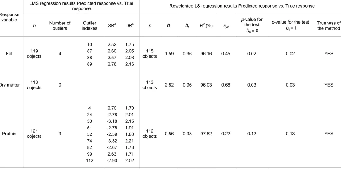
After a PLS model had been estimated for each of the three responses, a least squares (LS) linear regression was performed with the PLS predicted values of the response versus the values obtained by the corresponding reference method. Before the LS calibration, a LMS regression was carried out to detect possible outlier data caused by some kind of mistake occurred either at the construction of the PLS model or during analyses by the official method. The results of the LMS and LS regressions and p-values for the two hypothesis tests posed to check the trueness of every method are listed in Table 2. As p-values were higher than 0.01, it was asserted that, in all cases, the analytical behaviour of the PLS
function of the content provided by the respective official method are illustrated in Figs. 2a (fat), 2b (dry matter) and 2c (protein).
Detection capability for protein, dry matter and fat-to-dry matter ratio
In the chapter IV of [26], which lays down the regulations and specifications of Zamorano cheeses, the following physicochemical properties are established:
i) The protein content must not be lower than 25% in weight. ii) The dry matter content must not be lower than 55% in weight.
iii) The fat-to-dry matter ratio, expressed as percentage in weight, must not be lower than 45%.
In this context, the detection capability of every method at its respective minimum permitted level with α = β = 0.05 was estimated from the corresponding RLS regression performed previously. So, for each case and for a specific number of replicates, the operative curve of the hypothesis test (Eq. 4) was determined when α = 0.05. This graph shows the probability of false compliance, β, as a function of the percentage in weight of the corresponding response (protein, dry matter and fat-to-dry matter ratio) for its minimum level stated above. This nominal value is, in each case, that of x0 in Eq. 4.
For the percentage of total protein in Zamorano cheeses, several operative curves for the nominal minimum protein content of 25% are pictured in Fig. 3. Particularly, for α = β = 0.05, the decision limit, CDα, was 24.78% and the detection capability, CDβ, equalled 24.57% when 3 replicates were considered, curve (c). So the NIT-PLS-based method is able to distinguish 24.57% from 25% with probabilities of false non-compliance and false compliance equal to 0.05.
For the dry matter content, Fig. 4 collects four power curves for the minimum limit of 55%. With 3 replicates and α = β = 0.05, CDα, would be 54.14%, and CDβ, 53.28%, curve (c). The values for the dry matter percentage of the samples analysed ranged from 63.95 to 77.20%, all of them higher than the minimum percentage in law. This means that both CDα and CDβ were extrapolated values and for this reason they were overestimated. That is, the NIT-PLS based method is able to distinguish 53.28% from 55% with a probability of false
non-compliance equal to 0.05 and a probability of false non-compliance less than 0.05.
In the case of the fat/dry matter percentage, the PLS model which relates this variable to the SG (9,2,2)–SNV-pretreated spectra was first built instead of considering the ratio of the values obtained by PLS regression for fat and dry matter. According to the results of reference methods, percentages in weight of this ratio ranged from 49.96 to 59.87%. The evolution of the procedure designed to achieve the PLS regression is collected in Table 3, where it is shown that, after 11 outlier objects had been removed from the calibration set,the model that fitted the fat/dry matter ratio best was the one estimated from 8 latent variables (RMSEC = 0.43; RMSECV = 0.49; 92.54% of explained variance of the response). The mean, median and standard deviation of the absolute value of the relative error in calibration, which ranged from 0.03 to 1.98%, were, respectively, 0.66, 0.59 and 0.43%.
is equal to an error in the determination with PLS regression of the fat/dry matter ratio between 0.78 and 1.14%. However, if desired, the bias could be corrected using the Eq. (5)
PLS predicted
Lastly, the detection capability of the method for the fat-to-dry matter percentage at the minimum permitted level of 45% was estimated with α = β = 0.05. The operative curves determined for several numbers of replicates and α = 0.05 are depicted in Fig. 5. If 3
replicates were specifically considered and probabilities of false non-compliance, α, and false compliance, β, fixed at 0.05, CDα would be 44.39%, while CDβ would equal 43.78%, curve (c).
The true values of the fat/dry matter ratio were between 50 and 57.5%, higher than the minimum allowable quantity (45%) so, as in the case of the dry matter content, the
conclusion was that the NIT-PLS based method is able to distinguish 43.78% from 45% with a probability of false non-compliance equal to 0.05 and a probability of false compliance less than 0.05.
Acknowledgements
The authors thank the finantial support provided by Ministerio de Ciencia e Innovación (CTQ2011-26022) and Junta de Castilla y León (BU108A11-2) M.L. Oca is particularly grateful to Universidad de Burgos for her FPI grant.
References
[1] J.L. Rodríguez-Otero, M. Hermida, J. Centeno, J. Agric. Food Chem. 45(1997) 2815–
2819.
[2] J.L. Rodríguez-Otero, M. Hermida, A. Cepeda, J. AOAC Int. 78 (1994) 802–806. [3] M.M. Pierce, R.L. Wehling, J. Agric. Food Chem. 42 (1994) 2830–2835.
[4] C. Wittrup, L. Nørgaard, J. Dairy Sci. 81 (1998) 1803–1809. [5] D. McKenna, J. AOAC Int. 84 (2001) 623–628.
[6] T. Woodcock, C.C. Fagan, C.P. O'Donnell, Food Bioprocess Technol. 1 (2008) 117–129. [7] D.H. McQueen, R. Wilson, A. Kinnunen, E.P. Jensen, Talanta 42 (1995) 2007–2015. [8] M. Chen M, J. Irudayaraj, J. Food Sci. 63 (1998) 96–99.
[9] Da-Wen Sun, Infrared Spectroscopy for Food Quality Analysis and Control, Elsevier, 2009.
[10] P. Rolfe, Annual Review of Biomedical Engineering 2 (2000) 715–754.
[11] V. Tuchin, Tissue Optics: Light Scattering Methods and Instruments for Medical Diagnosis, SPIE Press, Bellingham (WA), 2000.
[13] R. Karoui, E. Dufour, R. Schoonheydt, J. De Baerdemaeker, Food Chem. 100 (2006) 632–642.
[14] C.M. Andersen, M.B. Fröst, N. Viereck, Int. Dairy J. 20 (2010) 32–39.
[15] R. Karoui, E. Dufour, L. Pillonel, D. Picque, T. Cattenoz, J-O. Bosset, Eur. Food Res. Technol. 219 (2004) 184–189.
[16] R. Karoui, J-O. Bosset, G. Mazerolles, A. Kulmyrzaev, E. Dufour, Int. Dairy J. 15 (2005) 275–286.
[17] E. Dufour, Int. J. Dairy Technol. 64 (2011) 153–165.
[18] S. De Angelis, R. Curini, M. Delfini, E. Brosio, F. D'Ascenzo, B. Bocca, Food Chem. 71 (2000) 495–502.
[19] R. Karoui, J. De Baerdemaeker, Food Chem. 102 (2007) 621–640.
[20] B.G. Osborne, in: Robert A. Meyers (Ed.), Encyclopaedia of Analytical Chemistry: applications, theory and instrumentation, John Wiley & Sons Ltd, Chichester, 2000. [21] H. Martens, T. Naes, Multivariate calibration, John Wiley & Sons, New York, 1989. [22] H. M. Heise, R. Winzen, in: H.W. Siesler, Y. Ozaki, S. Kawata, H.M. Heise (Eds.), Near
Infrared Spectroscopy: Principles, Instruments, Applications, Wiley-VCH Verlag GmbH, Weinheim, 2002.
[23] ISO 21543:2006 (IDF 201:2006) – Milk products – Guidelines for the application of near infrared spectrometry, first ed., International Organization for Standardization, Geneva, 2006.
[24] Council Regulation (EC) No. 510/2006 of 20 March 2006, Brussels, on the protection of geographical indications and designations of origin for agricultural products and
foodstuffs, Off. J. Eur. Commun. L 93 (31 March 2006) 12–25.
[25] Commission Regulation (EC) No. 1107/96 of 12 June 1996 on the registration of geographical indications and designations of origin under the procedure laid down in Article 17 of Council Regulation (EEC) No 2081/92, Off. J. Eur. Commun. L 148-I (21 June 1996) 1–15.
[26] Orden de 6 de mayo de 1993 por la que se aprueba el Reglamento de la Denominación de Origen “Queso Zamorano” y su Consejo Regulador, BOE No. 120 de 20 de mayo de 1993, 15311–15316.
[27] UNE–EN–ISO/IEC 17025:2005 – General requirements for the competence of testing
and calibration laboratories, International Organization for Standardization, Geneva, 2005.
[28] ISO 1735:2004 (IDF 5:2004) – Cheese and processed cheese products – Determination of fat content – Gravimetric method (Reference method), International Organization for Standardization, Geneva, 2004.
[30] ISO 8968–1:2001 (IDF 20–1:2001) – Milk – Determination of nitrogen content – Part 1:
Kjeldahl method, International Organization for Standardization, Geneva, 2001. [31] R.L. Wehling, M.M. Pierce, J. Assoc. Off. Anal. Chem. 71 (1988) 571–574. [32] R.J. Barnes, M.S. Dhanoa, S.J. Lister, Appl. Spectrosc. 43 (1989) 772–777.
[33] M.C. Ortiz, L. Sarabia, A. Jurado-López, M.D. Luque de Castro, Anal. Chim. Acta 515 (2004) 151–157.
[34] M.C. Ortiz, L. Sarabia, R. García-Rey, M.D. Luque de Castro, Anal. Chim. Acta 558 (2006) 125–131.
[35] R. Díez, M.C. Ortiz, L. Sarabia, I. Birlouez-Aragón, Anal. Chim. Acta 606 (2008) 151– 158.
[36] P.J. Rousseeuw, A.M. Leroy, Robust regression and outliers detection, John Wiley and Sons, New Jersey, 2001.
[37] M.C. Ortiz, L. Sarabia, A. Herrero, Talanta 20 (2006) 499–512.
[38] M.C. Ortiz, L.A. Sarabia, M.S. Sánchez, Anal. Chim. Acta 674 (2010) 123–142.
[39] J. Incédy, T. Lengyed, A.M. Ure, A. Gelencsér, A. Hulanicki, International Union of Pure and Applied Chemistry (IUPAC), Compendium of Analytical Nomenclature, Blackwell, Oxford, 1998.
[40]ISO 11843-2 Capability of Detection. Methodology in Linear Calibration Case, International Organization for Standardization, Geneva, 2000.
[41] Commission Decision 2002/657/EC of 12 August 2002 implementing Council Directive 96/23/EC concerning the performance of analytical methods and the interpretation of results. Off. J. Eur. Commun. L221 of 17 August 2002. Available in
http://eur-lex.europa.eu. Last visit: 2/04/2012.
[42] M.C. Ortiz, L.A. Sarabia, A. Herrero, M.S. Sánchez, B. Sanz, M.E. Rueda, D. Giménez, M.E. Meléndez, Chemom. Intell. Lab. Syst. 69 (2003) 21–33.
[43] M.C. Ortiz, L.A. Sarabia, I. García, D. Giménez, E. Meléndez, Anal. Chim. Acta 559 (2006) 124–136.
[44] R. Morales, L. A. Sarabia, M. C. Ortiz, Anal. Chim. Acta 707 (2011) 38–46.
[45] B.M. Wise, N.B. Gallagher, R. Bro, J.M. Shaver, W. Windig, R.S. Koch, PLS Toolbox 6.0.1., Eigenvector Research Inc., Manson, WA (2010).
Figure captions
Fig. 1 NIT spectra of the 124 Zamorano cheese samples in the original calibration set. On the X-axis, the spectral region (from 850 to 1050 nm). (a) Raw spectra. On the Y-axis, the logarithm of the inverse of the transmittance T of the sample. (b) Preprocessed spectra by means of the second derivative (9-point window, 2nd -order polynomial) of the spectra followed by a SNV transformation.
Fig. 2 Regression line of the values of each response calculated by its PLS model versus the values obtained by the reference methodology. (a) Fat content; (b) dry matter content; (c) protein content; and (d) fat/dry matter content.
Fig. 3 Probability of false compliance, β, versus protein percentage in weight
(probability of false non-compliance, α, fixed at 5%). (a) One replicate; (b) two replicates; (c) three replicates; and (d) infinite replicates. Nominal minimum value: 25% in weight.
Fig. 4 Probability of false compliance, β, versus dry matter percentage in weight (probability of false non-compliance, α, fixed at 5%). (a) One replicate; (b) two replicates; (c) three replicates; and (d) infinite replicates. Nominal minimum value: 55% in weight.
Protein
1st
(124) 9 100 95.73 115 (SR = -2.89) 0.30 0.36
2nd
(123) 9 100 96.02
77 (Qg = 0.02;
T2g = 23.92) 0.29 0.35
3rd
(122) 10 100 96.21 113 (SR = -2.55) 0.28 0.34
4th
(121) 10 100 96.57 0.27 0.33
(a) Latent variables.
(b) Root mean square error in calibration.
(c) Root mean square error in cross-validation.
(d) Absolute value of relative errors.
(e) Standard deviation.
(f) Standardized residual of data considered y-outliers.
Table 2. Results of the LMS and LS regressions performed with the values of each response calculated from the corresponding PLS model versus true values.
Response variable
LMS regression results Predicted response vs. True
response Reweighted LS regression results Predicted response vs. True response
n Number of
(a) Standardized residual of the object.
Table 3. Evolution of the development of the PLS calibration to evaluate the fat-to-dry matter ratio, expressed as percentage in weight, using the pretreated NIT spectra as predictors.
PLS model
(b) Root mean square error in calibration.
(c) Root mean square error in cross-validation.
(d) Absolute value of relative errors.
(e) Standard deviation.
(f) Standardized residual of data considered y-outliers.
850
890
930
970
1010
1050
1.6
1.8
2
2.2
2.4
2.6