Finite Gaussian mixtures and market risk assessment

Texto completo

(1)EGADE®. Business School TECNOLÓGICO DE MONTERREY. Hacemos constar que en la Ciudad de México, el día 12 de noviembre de 2014, el alumno:. Jorge Rosales Contreras. Sustentó el Examen de Grado en defensa de la Tesis titulada:. "Finite Gaussian Mixtures and Marketing Risk Assessment". Presentada como requisito final para la obtención del Grado de:. DOCTORADO EN CIENCIAS FINANCIERAS. Ante la evidencia presentada en el trabajo de tesis y en este examen, el Comité Examinador, presidido por la Dra. Linda Margarita Medina Herrera ha tomado la siguiente resolución:. Dra. Linda Margarita Medina Herrera. Lectora. Dr. Luis Vicente Montiel Cendejas. Director del Programa Doctoral. Lector. Calle del Puente No. 222 Col. Ejidos de Huipulco. Del. Tlalpan, México D.F., C.P. 14380. Tel. +52 (55) 5483-1766. www.egade.mx.

(2) Instituto Tecnológico y de Estudios Superiores de Monterrey Campus Ciudad de México. Finite Gaussian Mixtures and Market Risk Assessment. TESIS QUE PARA RECIBIR EL TÍTULO DE DOCTORADO EN CIENCIAS FINANCIERAS PRESENTA. Jorge Rosales Contreras. ~ ~cNOLÓQCO. • . DE MONTERREY. Director de tesis: Dr. Carlos Cuevas Covarrubias Lectores: Dra. Linda Margarita Medina Herrera Dr. Adán Díaz Hernández. México D.F., 12 de Noviembre de 2014. Biblioteca campuaCIIJdaddeMéxlco.

(3) .... ·-..,... .,._,,. ..

(4) En cariñosa memoria de . .. La maestra Anita y Don Saúl. En la ansiosa espera de Andreina Izel.

(5) Agradecimientos A Carlos Cuevas Covarrubias por sus atinados consejos durante más de dos años de trabajo a distancia y por no permitirme cejar en el intento. A Linda Margarita Medina Herrera y Adán Díaz Hernández por el tiempo dedicado a la revisión técnica de este documento y por su retroalimentación. A José Antonio Núñez Mora por confiar en que podría concluir el doctorado en ausencia.. A mis maestros, todos, por su pequeña en lo individual pero colectivamente significativa contribución.. A las instituciones que financiaron este proyecto:. ITESM Ciudad de México FIDERH del Banco de México Larrain Vial. A Rafael Flores, por su cuidadosa revisión de la redacción de este documento. Cualquier error remanente es de mi única responsabilidad. A los compañeros de trabajo que en estos últimos cuatro años, me permitieron ausentarme física y mentalmente sin mayor notoriedad. Destaco a José Antonio López, Ignacio Guzmán y Miguel Ángel González. En el plano personal, a mis hermanos Eduardo, Gabriel, Raúl, Javier y Anita por su respaldo incondicional y por hacerme sentir siempre en casa. Muy particularmente a mi esposa, Nayra González Durán, por su motivación, paciencia, comprensión y acompañamiento en los tiempos buenos igual que en los momentos de duda.. ii.

(6) Abstract Value at Risk (VaR) is the most popular market risk measure, as it summarizes in only one figure the exposure to several risk factors. Expected Shortfall (ES) corrects its limitations and has become a standard. Both measures can be estimated under different methodologies. The most commonly used are based on the empírica} distribution of asset returns or assume that they follow a Normal distribution. This assumption is not realistic in practice dueto the skewness and excess kurtosis observed in the actual behaviour of asset returns. In this work we introduce a comprehensive methodology to evaluate risk models that includes estimation, goodness of fit, risk estimation and model validation. Following that methodology we study and apply a parametrical model based on finite Gaussian mixtures, both stationary and autocorrelated. We derive a closed-form expression for ES and implement it estimating VaR and ES for a multi-asset portfolio. Performance vs usual models (Delta-Normal and Historical Simulation) is compared through backtesting. Evidence shows that the proposed model should be considered as a serious candidate for market risk assessment. A system of early risk alerts that allows to validate models without waiting to accumulate risk and profit and loss data is proposed and used.. Resumen El Valor en Riesgo (VaR) es la métrica de riesgo de mercado más popular, al resumir en una cifra la exposición a diversos factores de riesgo. El Déficit Esperado (ES) corrige sus limitaciones y ha ganado terreno. Ambas medidas se pueden estimar bajo distintos modelos. Los más comúnmente empleados se basan en la distribución empírica de los retornos de los activos o suponen que éstos siguen una distribución Normal. Este supuesto resulta inadecuado en la práctica debido a la elongación (curtosis) y asimetría observados en los retornos. En el presente trabajo introducimos una metodología para evaluar modelos de riesgo que incluye estimación, bondad de ajuste, estimación de riesgo y validación del modelo. Siguiendo esa metodología estudiamos y aplicamos un modelo paramétrico basado en mixturas Gaussianas finitas, tanto estacionarias como autocorrelacionadas. Derivamos una expresión cerrada para el ES y la implementamos estimando VaR y ES para una cartera multi-activos. Comparamos los resultados vs los modelos usuales (Delta-Normal y Simulación Histórica) mediante backtesting. La evidencia muestra que el modelo estudiado es un serio candidato para la evaluación de riesgo de mercado. También se propone y usa un sistema de alertas tempranas de riesgo que permite validar modelos sin necesidad de esperar a obtener una muestra significativa de datos de riesgo y resultado..

(7) Contents. Agradecimientos. ii. Abstract. iii. List of Figures. vii. List of Tables. viii. 1 Introduction 2. 3. 1. Normality Assumption in Finance 2.1 Derivatives Pricing . . 2.2 Portfolio Optimization 2.3 Risk Estimation . . . . 2.4 Limit Distribution .. 2.5 Mexican Market Data. 8. 9 9 12 13 14. Finite Mixture Distributions 3.1 Introduction . . . . . . . 3.2 General Mixtures . . . . 3.2.1 Basic Definitions 3.2.2 Interpretation . . 3.2.3 Moments of Finite Mixtures . 3.3 Finite Gaussian Mixtures 3.4 ldentifiabili ty . . . . . . . . 3.5 Estimation . . . . . . . . . 3.5.1 Method of Moments 3.5.2 Graphical Method 3.5.3 Maximum Likelihood . 3.6 Standard Errors . . . . . . . .. iv. 16 16. 17 17 18 19 21 25 29 29 31 32 35.

(8) Contents 4. 5. 6. 7. 8. V. Hidden Markov Models 4.1 Introduction . . 4.2 Definitions . . . 4.3 Markov Chains 4.4 Interpretation . 4.5 Moments of Markov Mixtures 4.6 ML Estimation of finite Markov Mixtures 4.6.1 Known States . . 4.6.2 Unknown States. 39. EM Algorithm 5.1 Introduction . 5.2 E Step . . . 5.3 M Step . . . . 5.4 EM for GM 5.5 EM for HMGM 5.6 Discussion . . . 5.7 Additional Considerations 5.7.1 Starting Values . . 5.7.2 Numerical lnstabilities .. 53. Goodness of Fit 6.1 Introduction . ..... 6.2 Q-Q Plots ... ..... 6.3 Kolmogorov-Smirnov. 6.4 Anderson-Darling. 6.5 Jarque-Bera. ...... 6.6 Discussion. ...... 6.7 Goodness of fit for unrestricted Gaussian Mixtures. .. 69. Market Risk using Gaussian Mixtures 7.1 Introduction . . . . . . . . . 7.2 Portfolio Loss Distribution . 7.3 Market Risk Measures 7.4 Backtesting ....... 7.5 Early Alerts . . . . . . . 7.6 Risk Model Estimation . 7.7 Model Validation 7.8 Discussion .. 80. Conclusions 8.1 Contributions 8.2 General Condusions. 39 40 42 44 46 49 49 51. 53 54 55 55 57 63 66 67 68. 69 69 70 73 75 76 79 80 81 83 87 90 93 95 97 100. . 100 . 101.

(9) Contents 8.3. Future Research. vi . . . . . . . . . . . . . . . . . . . . . . . . . . . . . . . . . . 103. A Proofs and Derivations A.l Convolution for Normal Distribution (Property 3.3). A.2 ES as Conditional Expectation (Proposition 7.4). A.3 ES for Normal Distribution . . . . . . . . . . . . .. 106 . 106 . 107 . 108. B Matlab Code B.1 VaR and ES for Gaussian Mixtures . B.2 Numerical Derivatives of Risk Measures B.3 Confidence Intervals for Risk Measures . B.4 Standard Errors for Estimators. 109 . 109. Bibliography. . 110 . 112 . 113. 115.

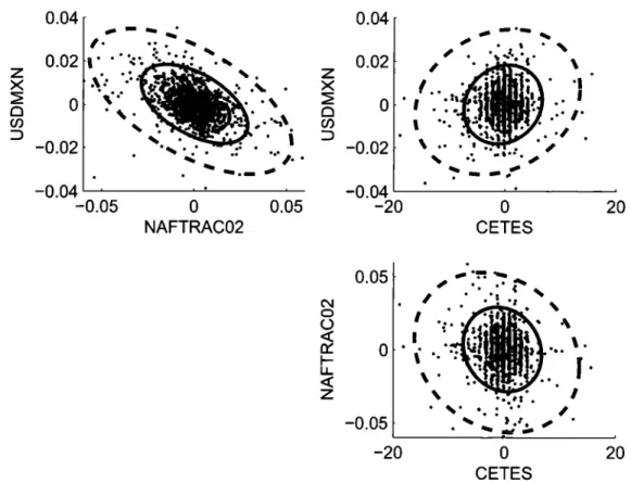
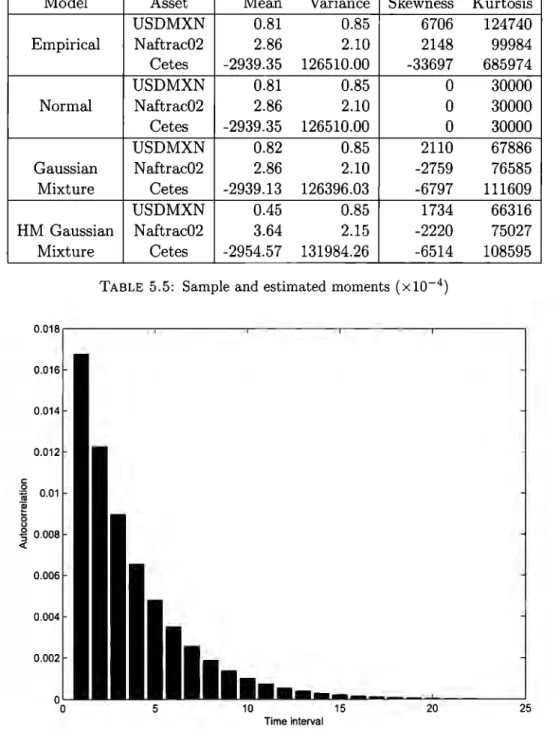
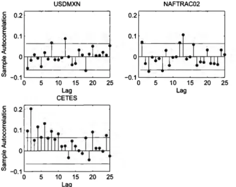
(10) List of Figures 2.1. Boxplots of Mexican Market Variables . . . . . . . . . . . . .. 14. 3.1 3.2 3.3. Arbitrary distribution approximation with Gaussian mixtures Financia! stylized facts reproduced with Gaussian Mixtures Volatility Regimes with Gaussian Mixtures. 23 23 24. 4.1. Regime Switching with Gaussian Mixtures .. 45. 5.1 5.2 5.3 5.4. Gaussian mixtures ellipsoids . . . . . . . . . Hidden Markov Gaussian mixtures ellipsoids . Autocorrelation function. . . . . . . Empirical Autocorrelation Function.. 57 64 65 66. 6.1 6.2 6.3 6.4. Normal Q-Q Plots . . . . . . Gaussian Mixture Q-Q Plots Interest rate CDF Plots . . . Interest rate GM CDF Plots.. 71 72. 7.1 7.2 7.3 7.4. Backtesting VaR(99%) . VaR(99%) Early Alerts VaR{99%) Early Alerts Backtesting ES{97.5%) .. 77 78. 97. 98 98 99. Vll.

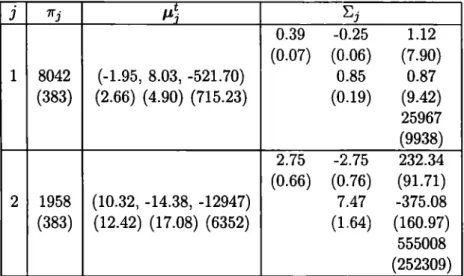
(11) List of Tables 2.1. EmpiricaJ Moments . . . . . .. 14. 5.1 5.2 5.3 5.4 5.5. Gaussian Mixture Estimators Hidden Markov Gaussian Mixture Estimators Hidden Markov Transition Probabilities Normal Distribution Estimators . Sample and Estimated Moments. 56 63 63 63 65. 6.1 6.2. Normality tests. . . . . . . . . Gaussian Mixture K-S tests ... 76 76. 7.1 7.2 7.3 7.4 7.5 7.6. Portfolio description. . . . . . Portfolio market value and sensitivities . Average VaR(99%) . Average ES(97.5%) . Backtesting VaR Backtesting ES .... 94 94 94 95 95 96. viii.

(12) Chapter 1. Introduction According to the Basel Committee, failure to capture major on- and off-balance sheet risks . . . was a key destabalising factor during the crisis. In response to the detected shortcomings. in capital requirements, the enhanced treatment introduces a stressed Value at Risk (VaR) capital requirement (see BCBS [6], paragraphs 11 and 12).. VaR, the most used market risk measure to estimate daily potential losses in either trading or investment books, was not able to grasp the extent of the sub-prime mortgage market collapse in the United States that triggered aggregated losses in market value over 130 billion (from February 2007) for firms such as Citigroup, Merrill Lynch, Morgan Stanley, UBS, among many others. This was mainly due to calculations based on historical simulations (heavily dependent on sample window) or debatable assumptions whose validity was often not even verified: the Senior Supervisors Group stated in 2008 that some firms' initial assessment o/ the true potential losses they faced were likely skewed downward by their VaR measures' underlying assumptions and a dependence on historical data from more benign periods [74].. Expected Shortfall (ES) is a coherent measure of risk (see Artzner et al [4]) and addresses the VaR limitations. In particular, it is sub-additive and tells the expected potential loss in case it exceeds VaR. Dueto its easy estimation under severa! distributional assumptions, is has become a standard.. 1.

(13) Introduction. 2. In spite of the above, VaR is still the most favored metric by institutions and regulators to monitor and control market risk (see, far instance, CNBV [19]) and the Basel Committee uses it to set minimum capital requirements. This Committee, however, has recently agreed to move from VaR(99%) to ES(97.5%) (see BCBS [7]). Many financia! models assume that -or are only tractable if- the returns of financia! assets are normally distributed. However, this assumption is usually not satisfied in practice. Empirical studies have shown that financia! returns frequently show lekptokurtosis or skewness, as well as volatility clustering. Befare applying any alternative model to estimate market risk figures, we have to quantitatively justify that the normality assumption is not fulfilled in practice. Far that matter, we review sorne popular -among the very many- normality test and apply them to sorne market variables. We consider these results suffi.cient to begin the search of a more adequate model.. More in general, we postulate a methodology far testing models that includes parameter estimation (with standard errors), goodness of fit testing, risk model estimation (again with standard errors) and model validation. This should be the standard approach to model testing , as it allows to identify its strengths and limitations. However, most authors skip the calculation of standard errors and many of them avoid testing far goodness of fit. A few even miss the now standard backtesting methodologies. Therefare, in presenting the family of finite Gaussian Mixture clistributions as an alternative candidate model to those most widely used in market risk estimation we fallow the proposed methodology. Not being a well-known model, we spend two chapters studying it in detail in the stationary and autocorrelated cases. First we introduce the family of finite mixture distributions with arbitrary component distributions. After sorne definitions, we interpret the finite mixture distribution framework in a way that proves to be useful: we can think of the mixture distribution as an incomplete data problem, where the component membership indicator of each sample point is not observable..

(14) Introduction. 3. In the specific case of finite Gaussian Mixtures, we review severa! of their particular properties, highlighting those that will be useful along this work. We show by means of graphical examples how they capture financia! stylized facts such as skewness, leptokurtosis and volatility regimes, provide a proof of the outstanding property of closedness under convolution and review three methods of parameter estimation; namely, a graphical method, method of moments and maximum likelihood. For the latter we also. show how to compute standard errors. The family of finite Gaussian Mixture distribution is very flexible but this flexibility comes at the price of a non-bounded likelihood function at sorne points in the border of the parameter space, making it somewhat difficult the process of maximum likelihood estimation. Then we relax the assumption of independence and identical distribution (iid) of the sample. The model is therefore extended to deal with dependent data, in particular, time series that display autocorrelation over time, captured through a stationary Markov process (an ergodic aperiodic Markov chain). The reason for this election is that the so called Hidden Ma.rkov Model (HMM) is a realistic model when the observations are collected sequentially in time and tend to cluster or alternate between different components (or regimes, therefore the name regime switching). Our contribution here consists in extending a result on persistence in Frühwirth-Schnatter [34] from two states to an arbitrary number of states as long as they are classified into two classes, or regimes. This idea can be useful to estímate the duration of a high market volatility episode.. In an analogous way to the stationary case, we formally define the Hidden Markov Model for finite Gaussian Mixture distributions (HMGM) and study sorne relevant properties, before going into the estimation of a Markov switching model via maximum likelihood.. Once we have intuitively supported the pertinence of the Gaussian Mixture model (either stationary or autocorrelated) we can proceed to apply the first steps of the proposed methodology, i.e., parameter estimation and standard error calculation..

(15) Introduction. 4. However, not only the likelihood function is not bounded, but also the likelihood equation <loes not admit a closed-form solution, so that it is important to devote a whole chapter studying the estimation algorithm under both situations: iid and autocorrelated samples. The Expectation-Maximization (EM) algorithm is a broadly applicable approach to the iterative computation of Maximum Likelihood Estimators in situations described as incomplete data problems. The ideas behind the EM algorithm are natural and intuitive, so that. earlier algorithms were applied in a variety of problems. However, the seminal paper by Dempster, Laird and Rubín [23] synthesized those ideas, provided a general formulation of the algorithm and investigated its properties. The basic idea of the EM algorithm is to associate the given incomplete-data problem with a computationally tractable complete-data problem. In the Expectation step (or E-step) we go from the observed the complete likelihood. Then the :.\1:aximization step (or M-step) maximizes the likelihood based on the completed data set. Starting from suitable initial values, E-step and M-steps are iteratively repeated until convergence, according to a preestablished criteria. We introduce the EM algorithm through the E and M-Steps and outline the algorithm for unrestricted finite Gaussian Mixtures and Hidden Markov Ga.ussian Mixtures. In both cases we illustrate the application of the algorithm with real data of the Mexican market and comment on the results. We also discuss sorne additional considerations on the implementation of the EM algorithm. One of the criticisms to the algorithm is that it <loes not automatically provide standard errors. So that as a contribution we have written Matlab functions to estímate those standard errors based on the empirical Information matrix as well as on the bootstrap for the two considered models. None of the functions is currently available as a standard function in the Statistics or Financia! toolkits in Matlab.. Continuing with the methodology we test the goodness of :fit of the Gaussian mixture to the same data that we used to reject the normality assumption. The evidence shows that at least the stationary version of this family of distributions is a good candidate to model.

(16) Introduction. 5. the returns of the market variables considered, besides interest rates, where a high number of components should be added to avoid rejecting the model.. The risk measures calculation (or model estimation) step is the most popular one as there exist vast bibliography (see below for a brief review). In orcler to be able to illustrate the application, we first derive the Portfolio Loss Distribution following the lines of McNeil, et. al. [57] and find the linear approximation through a loss operator that is efficient for small changes in the underlying risk factors. For the sake of completeness, we formally define the standard market risk measures to be calculated on the loss distribution and obtain their estimators under four different models, namely Historical Simulation, Delta-Normal, Delta-Gaussian Mixture and Delta-Hidden Gaussian Mixture. Our contribution here is a closed-form expression for the expected shortfall of a finite Gaussian mixture distribution, including its derivation. A particular case of our expression is used in Kamaruzzaman and Isa [41], where they estimate VaR and ES for monthly and weekly returns of a Malaysian stock index. We propose a multi-asset-type portfolio and estimate sensibilities to risk factors, fit multivariate Normal, stationary and autocorrelated Gaussian Mixtures distributions and estimate market risk measures (VaR and ES) under ali models, including Historical Simulation. We keep the Delta-Normal modelas benchmark only. In the context of risk management, Behr and Poetter [I l] model ten European daily stock indexes returns using hyperbolic, logF and mixtures of Gaussian distributions and conclude that the fit of the latter is slightly superior for ali countries in almost ali subperiods. Tan and Chu [77] model the returns of an investment portfolio using a Gaussian Mixture and estimate VaR. They also provide a proof of closedness under convolution for Gaussian Mixtures based on elementary calculus. Kamaruzzaman et.al. [40] fit a two--component Gaussian Mixture to univariate monthly log-returns of three Malaysian stock indexes. In a different work [41] they estimate VaR and ES (using an expression that is a particular case of (7.8) below) for monthly and weekly returns of and index and find, through backtesting that it is an.

(17) Introduction. 6. appropriate model. Zhang and Cheng [85] use Gaussian Mixtures with different number of components to estímate VaR of Chinese market indexes, bound it with the VaR of the components and link it to the behaviour of price movements and psychologies of investors. Autocorrelated versions of Gaussian Mixutres include Alexander and Lazar [2], who use the normal mixture GARCH(l,1) model for exchange rates. They find that a two-component model performs better than those with three or more components and better than Student-t GARCH models. Haas et al [36] introduce a general class of normal mixture GARCH(p,q) models for a stock exchange index. Their models have very flexible individual variance processes but at the cost of parsimony: their best models require from 17 to 22 parameters to model the returns of only one index. Hardy [38] fits a regime-switching lognormal model to monthly returns of two equity indexes and estimates VaR and ES using the payoff function of a European put option written on an index. Continuous versions of Gaussian Mixtures include the multivariate skew t distribution, the multivariate normal-inverse-Gaussian distribution or the multivariate generalized hyperbolic distribution and have been used by Lee and McLachlan [45] to model heterogeneous data with asymmetric and heavy tail behaviour. They find that those -infinite- component densities with four or more parameters can flexibly adapt to a variety of distributional shapes and compare favourably in the estimation of VaR to Gaussian mixtures, skew normal mixtures and shifted asymmetric Laplace mixtures, as they require a single component to accommodate the skewness and heavy-tails in the data. Their only drawback is that the interpretation of the parameters is not as intuitive as in the case of finite mixtures. Severa! other distributions have been used to model risk factors returns, such as nonsymmetric t distribution in Yoon and Kang [84], who find evidence suggesting that the skewed t distribution outperformed other symmetric distributions in describing accurate values of VaR models in Japanese financia! markets; or Generalized Error Distribution in Theodossiou [80], who find that empirical distributions of log-returns of severa! financia! assets at the daily, weekly, monthly, bimonthly, and quarterly frequencies possess significant skewness and leptokurtosis and attributes them to strong high-order moment dependencies..

(18) Introduction. 7. In order to select among models, we apply the model validation step, reviewing first backtesting procedures for each risk measure and then applying them to each asset and the portfolio. Both Gaussian Mixture models (stationary and autocorrelated) perform well at the portfolio level at all tested confidence levels and fail in sorne instances at specific combinations of asset and confidence level. The HMGM model <loes not seem to be superior to the stationary version.. In summary, in this work we propose the family of finite Gaussian Mixtures as an alternative model to fit risk factors returns distributions and estimate market risk metrics. This family preserves the parsimony of the normal model while explicitly capturing high volatility episodes through at least one of the components. Let us highlight that we provide evidence that it is a reasonable model for return distributions and market risk measures. We have used the normal model and historie simulation as benchmark models dueto the spread of their use, but we should warn the reader this is not an exhaustive or even ad-hoc model search. Previous versions of this work have been presented at the ASTIN, AFIR/ERM and IAALS Colloquia, Mexico 2012 by Cuevas and Rosales [22], the Conference of the International Federation of Classification Societies, Netherlands 2013 by Cuevas, Íñigo and Rosales [21], and the International Finance Conference, Mexico 2014 [67], and has been published in Rosales [68]..

(19) Chapter 2. Normality Assumption in Finance Many models used in quantitative finance assume that the returns of financia! assets are normally distributed. However, this fundamental assumption is usually not satisfied in practice. Empirical studies have shown that financia! returns frequently show lekptokurtosis or skewness (usually negative), as well as volatility clustering. For an early analysis, see Fama [29] who found sorne degree of leptokurtosis in every stock he analysed. He explains that, at the time, the classic approach to this problem was to assume that the extreme values are generated by a different mechanism than the majority of the observations. Still, he proposes stable distributions asan alternative to account for empirically observed leptokurtosis. On the other hand, Rosenberg [69] who found the existence of "highly significant extra-market components of covariance among security returns", attributed lack of normality to the likely existence of mixed normal return distributions.. In this chapter we review four common situations where either the models assume normality or practitioners apply them under the -maybe unnecessary- assumption that the underlying random variables follow a normal distribution. We finish introducing sorne data from the Mexican market that will be used throughout this work and revising an apology of the usage of the normal distribution in financia! modeling.. 8.

(20) Normality Assumption in Finance. 2.1. 9. Derivatives Pricing. The Black and Scholes [13] model assumes that the market consists of at least one risky asset, usually called the stock (S), and one riskless asset, usually called the money market, cash, or bond (with constant return r). It makes several assumptions on the assets, notably that it is a random walk (with drift, to be precise), i.e., that the instantaneous log returns behave as a Brownian motion, and that its drift and volatility (a) are constant. If they are time-varying, a suitably modified Black and Scholes formula can still be deduced, as long as the volatility is not random. The above assumptions imply that the returns follow a normal distribution and the prices. (V) follow a lognormal distribution. This allows to solve the price diffusion following differential equation. élV(t, St) at. +r. sªV(t, St). as. 2 ! 2s2 a V(t, St) -- V( S) _ O + 2a as2 r t, t -. in closed form. Due to the normality assumption, the Black-Scholes framework is unable to accommodate extreme moves in the asset returns, which practitioners hedge using outof-the-money options. It has other limitations, such as assuming that the volatility of the asset returns is constant. This can be overcome by adding t.he volatilit.y surface (implied volatility as a function of strike price and maturity) as risk factor, which in turn implies that its joint distribution with the asset returns should be normal. The same argument applies to the interest rate.. 2.2. Portfolio Optimization. Consider the allocation optimization problem. w*. = argmax:S(w), wEC.

(21) Normality Assumption in Finance. 10. where S is an index of satisfaction that depends on the investor's objective and C is a set of constraints. The objective is assumed to be a linear function of the allocation w an of the market prices vector (say M). In general it is not possible to solve this problem analytically, and even within the realm of numerical optimization, not ali problems can be solved. A broad class of constrained optimization problems that admit numerical solutions is represented by convex programming: in this framework S and C are convex (see for instance Boyd and Vandenberghe [14]). In ali the usual formulations (the objective can be absolute wealth, relative wealth or net profits), the investor's index of satisfaction is a functional of the distribution of the investor's objective. In turn, the distribution of the investor's objective is in general univocally determined by its moments. Therefore, S can be written in terms of the -infinite number ofmoments of the distribution of the objective. The Capital Asset Pricing Model (CAPM) builds on the model of portfolio choice developed by Markowitz (see [52] for a compilation of his work). In his model, an investor selects a portfolio at time t -. T. that produces a stochastic return at t. The model assumes investors. are risk averse and, when choosing among portfolios, they care only about the mean and variance of their one-period (of length r) investment return. As a result, investors choose mean-variance (MV) efficient portfolios, in the sense that the portfolios 1) minimize the variance of portfolio return, given expected return, and 2) maximize expected return, given variance. To say that investors only care about the first two moments of the objective means that they neglect all higher moments, so that the MV approach is an approximation unless S is a function of only the first two moments of the objective or the distribution of the market. M depends only on the first two moments. Let us analyze the index of satisfaction. The only case in which it depends only on the mean and variance of the objective is the certainty equivalent in the case of quadratic utility. u(y). 1 2 = y- -y 2(.

(22) Normality Assurnption in Finance. 11. as it has only two non-vanishing derivatives and the Taylor expansion consists of only three terms. Nevertheless this utility function is not flexible enough to model investor's preferences, as it violates the non-satiation principie (larger values of the objective make the investor happier), since u(y) is decreasing when y > (. There is also an additional issue of estimation error of the utility function parameters (( in this case) that can adversely affect optimality based on complicated or difficult to estimate parameters as described by Michaud and Michaud [60). Sharpe [75) and Lintner [50) added two key assumptions to Markovitz's model to identify a portfolio that must be mean-variance efficient. The first of those assumptions is complete agreement: given market clearing asset prices at t distríbution of asset returns from t -. T. T,. investors agree on the -true- joint. to t. See Fama and French [30) for an explanation. of the second assumption anda detailed discussion of the CAPM. Optimized portfolios, in this framework, begin with a specific utility function that defines satisfaction andan assumed return distribution. Besides quadratic utility, the only other case when the MV approach is an exact solution of the optimal allocation problem is when the distribution of the market prices M depends only on the first two moments. Even though sorne authors claim that this property holds for the entire family of elliptical distributions (see for instance Meucci [59), section 6.5) it is only the case of the multivariate normal distribution. Elliptical distributions depend on a location parameter, a scatter parameter and a characteristic generator that determines its tail behavior. This introduces additional parameters, such as the degrees of freedom in the case of Student-t. Moreover, Fang, Kotz and Ng [31) prove that a distribution is spherical (from which any elliptical can be recovered by a linear transformation) if and only if it is equal in distribution to a continuous homoscedastic Gaussian mixture. The single case when this equivalence <loes not introduce additional parameters is when the mixture is the Gaussian distribution itself (see section 3.3 below). In summary, a MV approach, including the CAPM, provides an exact solution of the optima} allocation problem under non-quadratic utility function only if the distribution of the market.

(23) 12. Normality Assumption in Finance. is normal.. 2.3. Risk Estimation. The value of an investment portfolio al time t, say factors {Zt E ffi.d):. Vi= f(t, Zt). Vi,. (see section 7.2 for more details).. Let us define the returns of the risk factors as Xt Lt. = -(Vi -. is a function of time anda set of risk. = Zt -. Zt-r and the portfolio loss as. Vi-r ). Then the linear approximation to Lt+r is. Lt+r ~ -. (. J(t, Zt) +. Zt) L 8f(t, az- Xt-T,j d. j=l. ). ,. J. where only the marginal returns Xt+r,j are random. If we assume that they jointly follow a d-variate normal distribution, then Property 3.3 (section 3.3) ensures that Lt+r is itself univariate normal and therefore risk measures such as quantile functions (VaR) or conditional expectations (ES) are a simple function of the parameters (see section 7.3). However, if we are in the presence of data that has heavy tails or excess kurtosis at least, and still fit a normal distribution for calculating VaR, then our VaR figure will underestimate the actual risk of the portfolio. A lower estímate of VaR leads to an insufficient capital maintained by the institution. Even if we switch the risk measure from VaR to ES, as suggested by the Basel Committee [7], under normality VaR. at 99% confidence leve} and ES at 97.5% confidence level are essentially the same, dueto the little mass of the normal distribution in the tails. The key property in this case is closedness under convolution. As opposed to the discussion in the previous section, the family of elliptical distributions is closed under convolution and the normal assumption is unnecessary. Moreover, this property also applies to the family of hyperbolic distributions, of which Gaussian mixtures is a particular case. We provide the proof of the corresponding property in section 3.3..

(24) Normality Assumption in Finance. 2.4. 13. Limit Distribution. Even if we do not assume that the relevant random variable follows a normal distribution, it is more often than not the case that the parameter we are trying to estimate is a nonlinear function of that relevant random variable, making its distribution simply infeasible to obtain. In such situation, and under certain conditions that may vary among instances, we can use the normal as a limiting distribution. Consider, for example, the following problem. The risk neutral valuation principle prompts that the fair value, say f(t,. Vi),. of a contingent claim with maturity-payment function h(Vr). is. ft(t, Vi) = Xt = EQ [exp (-r(T - t)) h(Vi)l$t], where Q is the risk neutral measure and $t is the u-algebra that contains all the information up to time t (see, for instance, Pennacchi [63], section 10.1). When it is not possible to calculate the conditional expectation above, it is still feasible to approximate it through the sample mean. ~ 1 n ft(t, Vi)=; ¿Xt,i. j=l. from realizations of a random sample {Xt,j}, j. =. 1, ... ,n. A conditional version of the. central limit theorem (see Grzenda and Zieba [35]) allows us to make the statement that the above estimator is asymptotically normal. Up to now, this is the only practica! way to value, for instance, an American put option -with many variations, of course-..

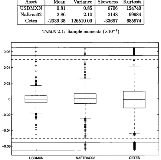
(25) Normality Assurnption in Finance. 2.5. 14. Mexican Market Data. In order to apply all the models and methodologies to be studied, we have taken a sample of 2700 daily returns, from 2003 to 2014 from representative variables of the Mexican financia! market, namely, USDMXN foreign exchange (FX), Mexican 6-month sovereign rate (Cetes) and Naftrac02 (an Exchange Traded Fund that replicates the behaviour of the Mexican Stock Exchange index). A subsample of it will be used for estimation purposes and the remaining will be kept for out-of-sample testing. At this point we present sorne exploratory analysis of the subsample: a boxplot in Figure 2.1 and the empirical moments in Table 2.1. Asset USDMXN Naftrac02 Cetes. Mean 0.81 2.86 -2939.35 TABLE. 0.06. 0.04. 0.02. Skewness 6706 2148 -33697. Kurtosis 124740 99984 685974. 2.1: Sample moments {xl0- 4}. I. +. 1. ------+-----------¡-----------~----+ --4--+. 1 1. j_. 1. o. 1:1 -0.02. Variance 0.85 2.10 126510.00. $. T. -0.04 .- - - - - -. ~. - - - - - - - - - -. a :. t-* ----------. i. -t-- - - - -. 1. -0.06. USDMXN. FIGURE. NAFTRAC02. CETES. 2.1: Boxplots of Mexican Market Variables. Table 2.1 shows that the empirical moments are notas those expected under the normality assumption. Even though the observed skewness does not seem to be a conclusive argument.

(26) Normality Assumption in Finance. 15. against normality, it is not the case of empirical kurtosis, which is from 3.3 times higher than that of the normal, for Naftrac02, to 22.9 times that benchmark for Cetes. Both features are confirmed in the boxplots in Figure 2.1, where the boxes look symmetric around the median, but the number of outliers (data points located further than 1.5 times the interquantile range from the median) is much more than expected under normality.. The simple exploratory analysis shows intuitive evidence against normality. However, the question of whether or not the normal distribution is appropriate in financia! modeling gives raise to endless debate. Esch (27] makes an apology of the normal distribution (not the normal assumption) arguing through the following lines:. • although financia! returns do not follow a normal distribution they do not follow any particular other family of distributions either, • alternative distributions are chosen more for their convenient properties of closure under convolution than for accurately describing returns, • the sources of variation should be modeled rather than substituting another incorrect distribution to directly model the data, • parsimony is preferable to complexity for out-of-sample performance.. He also advices that models under alternative distributions may have desirable properties in certain situations but they are often little known or not well-researched. They should be considered when there is a good reason why they are better than the standard set of models. In the following chapters we study, apply and test an alternative family of distributions that encompasses the normal, allows departures from it, models such departures and still preserves its parsimony..

(27) Chapter 3. Finite Mixture Distributions 3.1. Introduction. In this chapter we introduce the family of finite mixture distributions with arbitrary component distributions. After sorne definitions, we interpret the finite mixture distribution framework in a way that proves to be useful for parameter estimation purposes. We then review moments calculation based on the moment generating function. In the case of Gaussian Mixtures, we review several of their properties, highlighting those that will be important later on. We provide graphical examples of how they capture financial stylized facts such as skewness, leptokurtosis and volatility regimes. We provide a proof of closedness under convolution based on characteristic functions in a more general context than needed in finance. We also review three methods of parameter estimation for this model, namely, a graphical method, method of moments and maximum likelihood. For the latter we also show how to compute standard errors. We mainly follow the presentation of McLachlan and Peel [53], Frühwirth-Schnatter [34] and McNeil, Frey and Embrechts [57], but Everitt and Hand [28] and Titteringon, Smith and Makov [81] are also excelent earlier references.. 16.

(28) Finite Mixture Distributions. 3.2 3.2.1. 17. General Mixtures Basic Definitions. Consider a random vector X :. n. ---+ !Rd where the sample space. n. can be discrete or. continuous. Let X be characterized by its probability density function. f x(·) : JRd. ---+ JR+. which is a measurable function with respect to either Lebesgue measure or a counting measure.. Definition 3.1. Let X :. n. ---+ JRd be a random vector. We say that it follows a finite. (g-component) mixture distribution if its density function can be written as 9. /x(x). = L 1rj/j(x) Vx E !Rd, j=l. where gis a positive integer, /j : JRd---+ JR+,j 1, ... , g are positive constants such that. =. {3.1). 1, ... ,g are density functions and 7rj,j. =. L}=l 7rj = l.. The number of components g will be considered fixed for our purposes, but in many applications its value is another unknown parameter to be estimated. The densities /j are called component densities, the constants 7rj are known as rnixing proportions or simply, weights and the vector. 7r. 1. = (1r1, ... , 1r9 ). is the mixing or weight distribution. Since. Ji are. densities, it is clear that the mixture density f x is well defined. Component densities are usually assumed to come from the same parametric family, although this is not necessarily the case. We will drop the subscript X whenever there is no confusion that. f. refers to the. mixture density. Dueto linearity of the integral, Definition 3.1 may be written in terms of cumulative distributions functions or even characteristic functions (or moment generating functions), instead of densities..

(29) Finite Mixture Distributions. 3.2.2. 18. Interpretation. The following statistical problem where a finite mixture distribution arises in a natural way was first noted by Feller [32] and will prove to be very useful for estimation purposes in section 3.5.3 below. Considera population made up of g non-overlapping subgroups, mixed at random in proportions. 1r 1 , ... , 1r .. 9. Assume that interest líes in sorne random fea.ture X which is heterogeneous. across the groups and homogeneous within them. Due to heterogeneity, X has a different probability distribution in each group, say Jj(Xl8), where the vector parameter 8 contains the specific parameters for all groups. The groups may be labeled through a discrete indicator vector Z taking values in the set {O, 1 }gxn, where n is the sample size:. .. _ { 1, if Xi carne from the jth component Z Ji O, otherwise. .. When sampling randomly from such a population, we may record not only X, but also the group indicator Z. The probability of sampling X from the group labeled j (which means Zj.. = 1) is equal to 7rj, whereas conditional on knowing Zj.,. X is a random vector following. the distribution fi(Xl8i) with 8j being the parameter vector in group j. The joint density. f(X, Z) is given by. J(X, Z) = f(XIZ)p(Z) = fi(Xl8i)rri. A finite mixture distribution arises if it is not possible to record the group indicator vector Z; and only the random feature X is observable. Summing over ali possible values of Z the. marginal density f(X) is clearly given by the mixture density (3.1). More formally, let us assume that the random vector X is defined over a sample space. n. and follows a g-component mixture distribution.. The intuitive interpretation above. translates into the existence of a partition {D 1 , n 2 , ... D9 } of the sample space rrj. = Pr(Dj),j = 1, ... ,g. Component densities fi,j. n,. where. E {1, ... ,g} correspond to conditional.

(30) Finite Mixture Distributions. 19. probability densities of X given Ü.j,j E {1, ... ,g} respectively. In this case, the posterior probability of ni given a realization x of X, is. There are also many examples in practice where the components can not be identified with exogenous groups as above, so that the components are introduced into the mixture to allow for flexibility in modeling a heterogeneous population that is unable to be modeled by a single component distribution. The extreme of this exercise is the nonparametric kernel estimate of the sample density. In this fashion, if the number of components in the mixture equals the sample size (g ali weights are 1/n, and we make Jj(x). = ik(x~xi). = n),. for some kernel density function k(-). and bandwidth parameter h, we can think of the mixture distribution as the nonparametric kernel estimate of a density function (see McLachlan and Pee! [53], section 1.4).. 3.2.3. Moments of Finite Mixtures. For the same reason noted at the end of section 3.2.1, moments of finite mixture distributions are easily available, as long as the moments of the component distributions exist. Indeed, to determine the expectation of a function H(X) of the random vector X, we can write. E (H(X)) =. 1. H(x)fx(x)dx =. n. 9. L 1íjEh (H(X)),. (3.2). i=l. where Eli denotes expectation with respect to the density Í:,'. Let H(x) = exp {t'x}, then G(t) = E (H(X)) is the moment generating function of the random vector X, which has as many finite moments as derivatives around zero the function G(t) has. For instance, it is easy to see that.

(31) 20. Finite Mixture Distributions. g. µ = E(X) = G'(t =O)=. L 1íjµj,. (3.3). j=l. provided that all the component means µ 1 =. fn x/j(x)dx exist.. In the univariate case, higher arder moments around zero (raw moments) are easily obtained from the corresponding moments of the component densities:. g. µk. = E(Xk) = c(k)(t =o)=. L. 1µj,. 1r. (3.4). j=l. Central moments are obtained from E (H(X)) with H(X). = (X-µ)k and Newton's binomial. formula. g. =. L rr1E1; ((x - µj + µj -. -t t. G). µl). j=l. "i. If k. = 2,. (µj - µ)'-' El; ((X - µj)').. (3.5). for example:. ª2. =E. ,,. g. j=l. j=l. L 1íjaJ + ¿ ·rrj(µj - µ)2. =. ((X - µ)2). g. ". E1r(aJ). + Var1r(µ1),. i.e., the variance of the mixture is the mean of the component variances plus the variance of the component means, both computed with respect to the mixing distribution. In other words, the variance of the mixture distribution captures the within component dispersion as well as the between components dispersion. Higher central moments are:.

(32) Finite Mixture Distributions. 21. g. cr- 3 E ((X - µ) 3 ). = cr- 3 ¿. 7rj. [(µj - µ) 2 + 3crJ] (µj - µ),. (3.6). j=l g. cr- 4 E ((X - µ) 4 ) = cr- 4. L 1íj [(µj - µ). + 6(µj. 4. - µ) 2 cr;. + 3crJ].. (3.7). j=l. 3.3. Finite Gaussian Mixtures. The mixture of two univariate arbitrary normal distributions is the oldest known application of a finite mixture distribution (Pearson [62)), where he fitted by the method of moments this model to a dataset of crab measurements. In this section we define such mixtures and review sorne specific properties and results to be used later on.. Definition 3.2. We say that a random vector X ~. follows a finite Gaussian Mixture. ]Rd. distribution if its density function is a mixture of d-variate normal densities:. where {rri}}=l are as in the previous definition, µi E matrices for each j. !Rd. and Lj E. !Rdxd. are positive definite. = 1, ... , g.. From equation (3.2) we can obtain the characteristic function of the finite Gaussian Mixture distribution, making H(x) = exp{it'x}, where i =. 1/Jx(t). =. t. J=l. where 1PX; (t). = exp {. it'. µi -. 1ri exp. {it'. v'=T:. µi -. ~t'Eit}. {3.9). ½t'Eit} is the characteristic function of the jth multivariate. normal component. This function will be useful in the proof of several properties below..

(33) Finite Mixture Distributions. 22. From {3.6), it is clear that the distribution is skewed if at least two of the component means are distinct. From {3.7) and assuming g = 2 for illustration, if µ1 = µ 2 and cr1 #- cr2 then the mixture distribution has fatter tails than a normal distribution.. In fact, Teicher {[78]) proves that a finite mixture of distinct Gaussian components can not be Gaussian. More in general, it is not difficult to see that the mixture of exponential family components with unrestricted parameters is not in the exponential family. Besides the above, the family of finite Gaussian Mixture distributions displays the following properties:. l. it encompasses the Normal distribution (with g. 2. as noted in section 3.2.2, if g. =n. = 1),. and under additional assumptions, we can think of. the mixture distribution as a nonparametric model, 3. for intermediate cases (1. < g < n) the mixture model can be seen as a semiparametric. model that is able to approximate any continuous distribution (see Figure 3.1), 4. its elements may be very flexible: a g-component univariate Gaussian Mixture distribution can be defined using up to 3g - 1 parameters (dg(d. + 3)/2 + g -. 1 in the. d-variate unrestricted case), and it can be used to model a continuous distortion of the normal -skewness, leptokurtosis, contamination models, multi-modality, etc- often with g. = 2 only (see McLachlan and Peel [53], section 1.5).. 5. it has an infinite number of moments. This can be either an advantage or a limitation, as heavy-tail 1 distributions are not properly modeled. 6. it is not difficult to simulate, so it can be used in MonteCarlo or bootstrap processes. 7. it matches financia! stylized facts (as opposed to other distributions like Student-t or hyperbolic), such as skewness and leptokurtosis (see Figure 3.2), but markedly market volatility regimes (see Figure 3.3). 1. For clarity, we understand that the distribution of a random variable X has a heavy right tail if limx--++oo eÁ"' P(X > x) = O. See Asmussen [5] for the definition and Klugman, et. al. [43] for a deeper discussion of tail behavior.

(34) 23. Finite Mixture Distributions 8. it is closed under convolution.. 0.4 - - Studenrs t - - - 3-component GM · 2-component GM - · - 1-component GM. 0.35. 0.3. 0.25. 0.2. 0.15. 0.1. 0.05. o-4. -3. -2. o. -1. 2. 4. 3. FIGURE 3.1: Arbitrary distribution approximation with Gaussian mixtures. 0.4. 0.4. 0.35. 0.35. 0.3. 0.3. 0.25. 0.25. 0.2. 0.2. 0.15. 0.15. 0.1. 0.1. o.os. o.os. ' ..... ., / -4. -2. o (a). 2. 4. \. /. 6. o. -6. -4. -2. o. ' 2. 4. 6. (b). FIGURE 3.2: Financia! stylized facts reproduced with Gaussian mixtures: (a) skewness with 0.35N(-1,4)+0.65N(l,l) and (b) leptokurtosis with 0.85N(0,1)+0.15N(0,9). Normal density with same mean and variance (dotted line) plotted for comparison.. The last property is very important and will be used in section 7.3 to obtain aggregated risk measures. Since it inherits this property from the Normal distribution, we state it for.

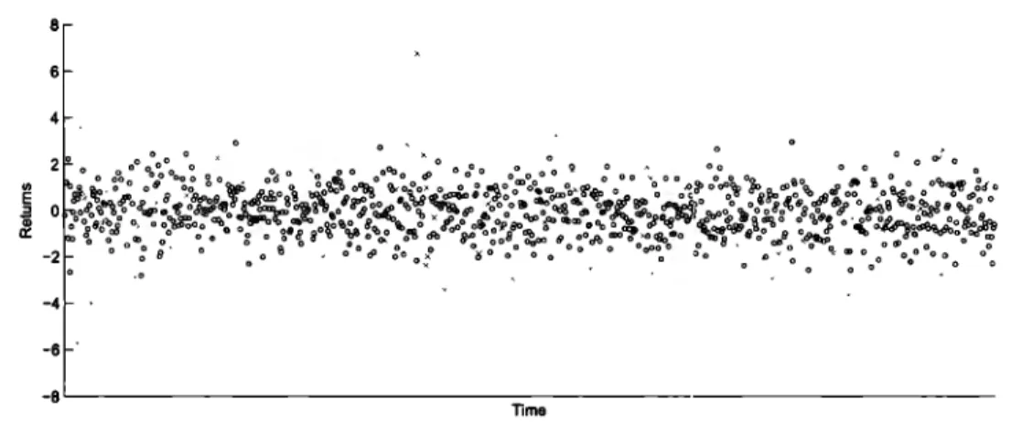
(35) Finite Mixture Distributions. 24. 8 6 4. -4. -6. -8'-----------------------------Time. 3.3: Volatility regimes with Gaussian mixtures: random sample from 0.85N(0, 1)+ 0.15N(0, 9). Circles come from first component and x-rnarkers from second one.. FIGURE. both distributions and assign them a number for later reference. The proof of the first one can be found in McNeil, et. al. [57] and makes use of characteristic functions. We include below the proof of the second, because of its relevance to our work.. Property 3.3. (Normal case) lf X ,. ._, Nd(µ, E) and l(:i:) N(µ¡, u¡), with µ¡. = -(c + w' µ). and u¡. =w. 1. = -(c +. w' :i:), then l(X) ,. ._,. Ew.. Property 3.4. (Gaussian Mixture case) lf X,..._, GMd(1r, {µj };=l, {Ej}J= 1 ), 1r, µj E JR.d,. = 1, ... ,g with µ¡ 1 = - (c + w'µj). Ej E JR.dxd, j. and l(:i:). =. -(c+w':i:), then l(X) ,..._,. and u½= w'Ejw,j. GM(1r,{µ1JJ= 1,{u½}]= 1),. = 1, ... ,g.. Proof. In a slightly more general context, let Y= WX. + e,. W E JR.kxd, e E JR.k, then the. characteristic function of Y is. 7h(t). since the characteristic function of X is given by (3.9). Therefore.

(36) Finite Mixture Distributions. Making k. 25. = 1 completes the proof of the Property, as we can see that in this case Y= -l(X), D. As immediate consequence of Property 3.4, we have that the marginals of a multivariate Gaussian mixture distribution are also Gaussian mixture distributions in the corresponding dimension: to obtain univariate marginals, for instance, make e = O and W =e'E JR.lxd, where e is any of the canonical vectors in JR.d.. j cu. "O "O co "O. ~. A second important consequence of this Property is that the sum of two d-variate random. ü. 11). vectors with Gaussian mixture distribution follows again a d-dimensional Gaussian mixture distribution. To see this, Let X and V be random vectors in JR.d, form the vector (X, V)' E JR. 2d and make e= O E. JR.d. and W. = ~d Id]. E JR.dx 2d, where Id is the d x d identity matrix.. Then Y= [Id Id](X, V)'+ O= X+ V is a d-variate Gaussian mixture. This implies that the Gaussian mixture distribution is infinitely divisible, a very useful property in financial modeling, since log-retums can be easily projected from a given estimation period (say daily, for instance) to a differeµt investment horizon (weekly or monthly, for instance). In summary, finite Gaussian mixtures provide a straightforward, still very flexible, extension of the usual Gaussian model. The price to be paid for this flexibility is that their inference results in complex computational problems, as discussed in section 3.5.. 3.4. ldentifiability. Before addressing the estimation of finite mixtures, we have to take sorne time to review the issue of identifiability of a mixture distribution, that will be essential for parameter. ~. c.. ns u. cu a ...,0 E. ( ·--·-.e. 1: o l:. cu ou. "O. ~g o. ~. ra.

(37) Finite Mixture Distributions. 26. estimation. As an example, consider the very simple situation of a two-component homoscedastic univariate Gaussian mixture f(x). = 1r<J,((x -. µ¡)/u). + (1. - 1r)<J,((x - µ2)/u).. way to distinguish between the two different parameter vectors. e~ = (1 -. There is no. e~ = (1r, µ 1, µ2, u). and. 1r, µ 2 , µ 1 , u) as they describe the same density.. Consider, further, the case of a univariate mixture of two normal distributions with arbitrary parameter 0. = (1r, 0) and density /(xl8).. Any mixture of two normal distributions may be. written as a mixture of three normal distributions by adding a third component with weight. 1r3. = O.. The parameter '11. density /(xl'11). = (1r,O,0,µ3 ,u~) is clearly different from 8 but defines the same. = /(xl0).. Let us formally define identifiability and then review the three types of nonidentifiability distinguished by Früwirth-Schnatter [34], addressing also how to overcome them.. Definition 3.5 (Identifiability). A parametric family of distributions, indexed by a parameter 0 E 0, defined overa sample space n, is said to be identifiable if for any two parameters. 01 and 02 in. e,. f (xl01) = f (xl02) for almost all x E IR<=} 01 = 02.. Invariance to Component Permutation. Nonidentifiability of a finite mixture distribution may be caused by the invariance of a mixture distribution to relabeling the components, as first noted by Redner and Walker. [66]. Consider a mixture of two Gaussian distributions with parameter vector (1r1, 1r2, 81, 82) where 1r1 =/= 1r2 or 8 1. =/: 82. Then the distribution induced by the parameter (1r2, 1r1, 82, 81). is the same even though the parameters are clearly different..

(38) Finite Mixture Distributions. 27. For the general finite mixture distribution with g components defined in (3.1), there exist g! equivalent ways of arranging the components. Each of them described by a permutation of the set {1, ... , g}. Because of this, a finite mixture distribution is not strictly identifiable in the sense of Definition 3.5.. Overfitting. Considera finite mixture distribution with g components, defined in equation (3.1), where. (1r1, ... , 1r9 , 81, ... , 89 ) E 0 9 . Consider now a finite mixture distribution from the same parametric family, howev_er, with g - l components. Crawford [20] shows that any mixture with g - l components defines a nonidentifiability subset in the larger parameter space 0 9 , which corresponds to mixtures with g components, where either one component is empty or two components are equal. This situation if of utmost relevance when dealing with mixtures with an unknown number of components. Due to this type of nonidentifiability, one should exercise maximum care when fitting finite mixture distributions by starting with n(=sample size) components and then pruning the number of components.. In the two situations above, formal identifiability is achieved by constraining the parameter space. e. in such a way that the density (3.1) is assumed to be a mixture of g distinct,. nonempty components:. • An inequality condition on the component parameters avoids nonidentifiability due to permutation of the components. For mixtures with a multivariate component parameter the arder is partial and should be required to the mixing distribution. 1r. or. to single entries of the vectors 8i. This is not sufficient for all situations as noted by Frühwirth-Schnatter [34] but it worked out in all the cases we dealt with. • A strict positivity constraint on the weights avoids nonidentifiability due to empty components..

(39) Finite Mixture Distributions. 28. General nonidentifiability. Finite mixture distributions may remain unidentifiable, even if a formal identifiability constraint rules out any of the nonidentifiability problems described above. A well-known example of a nonidentifiable family is finite mixtures of uniform distributions (see, for instance, Everitt and Hand [28]). A second example is finite mixtures of binomial distributions (Titterington et al. [81 ]). Generic identifiability of finite mixtures of distributions is a class property and has to be defined (see Yakowitz and Spragins [83]).. Definition 3.6 (Generic Identifiability). Consider two arbitrary members of the class of finite mixture distributions T(8) with deilsity /(-18) indexed by a vector parameter 8 E 0: 9*. g. ¿. 1rjT(8j) and. j=l. ¿. 1rJT(8J).. j=l. Assume that the formal identifiability conditions discussed above are satisfied. The class of finite mixtures of distributions T( 8) is said to be generically identifiable, if almost everywhere (a.e.) equality of the mixture density functions g. 9*. j=l. j=l. L 1íj/(-l8i) = ¿ 1rJJ(-l8J) a.e. implies that g. = 9*. and that the two mixtures are equivalent apart from re-arranging the. components.. Teicher [79] proves that many mixtures of univariate continuous densities, especially univariate mixtures of normals, are generically identifiable. These results are extended by Yakowitz and Spragins [83] to various multivariate families such as multivariate mixtures of normals..

(40) Finite Mixture Distributions. 3.5. Estimation. Let X'. =. 29. (X1, ... , Xn) be a set of independent and identically distributed (iid) random. variables following a finite Gaussian mixture distribution. As usual, we will denote with. =. small caps a realization of the random variables: x'. (xi, ... , Xn)- Let 81. 1, ... , g be the vector of parameters of the component densities, where 8j vector of parameters of the jth component, and :Ej is understood to be case. Let E>' 1r'. =. = {8j },. j. =. = (µj, Ej )' is the. a} in the univariate. (-rr, 0) be the set of parameters of the finite Gaussian mixture, where. = (1r1, ... , 1r9 _i) dueto the restriction in Definition 3.1.. In this section we briefly review the estimation of E> vía method of moments and a graphical method, to later concentrate on maximum likelihood. Other common approaches not discussed here include minimum-distance methods and Bayesian estimation.. 3.5.1. Method of Moments. The estimation of finite Gaussian mixture parameters using the method of moments dates back to the nineteenth century (Pearson [62]). The standard approach consists of equalising the sample moments with the theoretical ones obtained in (3.4). In the univariate case this reads:. 1. ffij. j. .. 9. .. .. = -n I: xf = I: 11"iµt = µ1, j = i, ... , k. i=l. (3.10). i=l. Each equation is typically nonlinear in the elements of E>. The estimation procedure requires solving the above system of k equations and r unknowns, where r is equal to the dimension of E>. In the unrestricted case r = 3g - 1, so that if k. < 3g - 1, there exist free parameters. and the problem of finding the "optimal'' solution arises. On the other hand, if k. > 3g - I. there could exist no solution. In Pearson's pioneering work he estimated the five parameters of a two-component univariate heteroscedastic Gaussian mixture by solving a ninth-degree polynomial, which in his time was regarded as a "heroic task" (Charlier [18]). Efficient method-of-moments estimators.

(41) 30. Finite Mixture Distributions. include Lindsay [48] for univariate mixtures and Lindsay and Basak [49] for multivariate ones. For the specific case g. = 2 Lopez de Prado and Foreman. [51] recently introduced a method. that exactly fits the first three sample moments and uses the fourth and fifth moments to choose among available solutions. They call this procedure the EF3M algorithm (Exact Fit of 3 Moments).. Algorithm 3. 7. (Method of Moments: EF3M). 1. Calculate 5 sample moments around zero, say m1, ... , m5 from (3.10). 2. Assume µ2 as given (µ2. = m1, for instance).. 3. S elect randomly 1r E (O, 1).. 4- Set k. = O and assign 80 = (1r,m1,µ2,m2,m2)'.. 5. Estímateµ¡ by µ1. = ¼[m1 -. 6. Solve the system Au. (1 - 1r)µ2].. = b for u'= 1-. (cr1, cr2) with. 7r. ]. 3(1 - 1r)µ2 · ~ A- 1 b. i.e., u=. 7. Estímate µ2 from m4 by ~. µ2. =. l. [. 1 1/2 - 3CT22 1/ 4 m4 - 1r(3cr41 + 6µ 21cr 12 + µ 4)) ( 6 CT2 + ----'----==----..::......;=------='-"-. 1-. 8. Estímate the mixing proportion as "1r. 7r. = "":i_s__--/,. I. where. a -- 5µ 1cr41 + 10µ 31cr 12 + µ 51 an d. 2.

(42) Finite Mixture Distributions. 31. 1O. Calculate convergence criterion. 11. lf error>. f.. for a given threshold. €,. add 1 to k and go back to step 5, otherwise, end.. Sorne potential difficulties with the algorithm include that if µ1 and µ2 are clase to each other or if 1r1 ~ 1 then the estimation of cr~ produces an indetermination, while if 1r1 ~ O then µ 1. ~. oo. In addition to that, it is possible to get negative estimations for the variances. or values outside the [O, 1] interval for the mixing proportion. Due to the calcula.tion complexities and potential difficulties as those signaled above, method of moments estimators are not usually input as initial values in iterative estimation procedures such as maximum likelihood.. 3.5.2. Graphical Method. In between the almost intractable method of moments and befare computers allowed the iterative implementation of maximum likelihood, Bhattacharya [12] proposed a graphical method to salve the problem of identifying the number of components of a univariate mixture of normal distributions when the means are sufficiently separated, as well as to estímate the parameters of each component. The fundamental assumptions are: i) the components are sufficiently separated, in the sense that for each component there exist a region where the effect of the rest of the components is negligible, and ii) the class interval is sufficiently small. The rationale behind the above assumptions is that, on the one hand, the data from each class will be used to estímate parameters of a single component and, on the other hand, the error of the approximation depends on the length of each interval. The algorithm is as follows:. Algorithm 3.8. {Graphical Method).

(43) Finite Mixture Distributions. 32. l. Group the sample in m classes of constant length h and get middle class points (xj). and frequencies (Yi) for each class. 2. Plot Ir (r. ~ log(yj) =. = 1, ... , g). log(yi+ 1 ). -. log(yj) against xi (j = 1, ... , m) and look for regions. where the graph looks like a negative-slope straight line segment.. 3. The number of identified line segments (g) is the number of components.. 4- Calculate the slope (tan fJr) and the interception (Ar) of each line segment. 5. Calculate the parameter estimators of each component: µr = Ar. + h/2,. and a; =. hcot 0r - h 2 /12. 6. Estímate mixing proportions as 'Trr = nr/ ¿¡= 1 ni, where nr = ¿iElr yif ¿iElr Pr(xi) and Pr(x). 3.5.3. = cI>((x + h/2 -. µr)/ar) - cI>((x - h/2 - µr)/crr)-. Maximum Likelihood. Assuming that the dataset is the realization of iid random variables, the log-likelihood function of a multivariate g-component Gaussian Mixture is. (3.11). The first hurdle that one has to take into account is that the likelihood function is unbounded. Indeed, from the form of the density (3.8) if any of the data points Xj happens to be equal to any of the component means µi (it <loes not have to be its own mean, i and. j can be different) while at the same time. IEil. -+ O, then the likelihood goes to inifinity.. So the global maximum <loes not exist and one has to content oneself with finding a local maximum. Even in this situation, taking derivatives with respect to. 'Tri,. (i. = 1, ... , g -. 1). and equalising to zero:. (3.12).

(44) Finite Mixture Distributions. 33. it is clear that it is not possible to obtain a close-form solution for the elements of 8. Therefore, based on the interpretation discussed befare, we approach the problem as a censored sample, where the complete sample is. .. _ Z iJ -. Xe. = (x', z')' but the membership variable. 1, if x 1 carne from the ith component. {. O, otherwise (i = 1, ... , g; j = 1, ... , n) is not observable. So the log-likelihood of the complete (unobservable) sample is:. n. log Le (8). g. =L L. log (1ri</> (x1 ; 0i)). Zij. j=l i=l. n. =L. n. g. L. log7ri +. Zij. j=l i=l. n. =L. l n. g. L. Zij. log 7ri -. j=l i=l. Observe that. g. LL. Zij. log</> (x1; Oi). j=l i=l. 9. 2L L. Zij. [dlog(27r). + log IEil + (xj -. µd. 1. E¡ (xj -. µi)].. j=l i=l. ¿f= 1 Zij = 1 for each j = 1, ... , n,. n. log Le (8). =L. g. therefore:. L Zij log 7ri -. d. ~ log(21r) -. j=l i=l. 1. -2. n g LLZij. [loglEil. + (x1 -. 1. µi)'E¡ (xj. -µi)].. (3.13). j=l i=l. Obtaining the Maximum Likelihood Estimators (MLEs) involves calculating derivatives from equation (3.13) with respect to each parameter, equalising to zero and solving the resulting system of equations. The derivative with respect to mixing proportions is.

(45) Finite Mixture Distributions. 34. ~logLc(E>) 01íi. =. t .. J=l. [Zij 1íi. Zgj] 1íg. = O,. (3.14). = 1, ... ,9 -1, which is much easier to solve than (3.12). Let us first observe that this equality holds also for i = g. Indeed, multiplying (3.14) by 7ri we obtain. for i. n[ ] 7íi L Zij - ;-Zgj j=1. = o {::>. L. gn L Zij. lgn L 1íiZgj•. = ;- L. i=1 j=l. g. g i=1 j=l. Interchanging the order of summation and using that. l. n. = l and. ¿f=I 7ri =. 1:. l. n. ¿1 = -1í ¿ z g j j=1. ¿f=I Zij. =}. 7f9ML. n ¿zgj· n .. =-. g j=1. J=l. Substituting this expression in equation (3.14):. n. l. n. ¿ z i j = 1íi ¿ z g j = n1ri 7r j=1 g j=1. The process for. µi. =}. 1riML. n. = -n.¿ z i j , i = 1, ... ,g-1. J=l. and Ei is more straightforward:. l. n. 1 -- ~2z--E:L...,¿ lJ i (x·1 - µ-)=O i. 2. {=>. L. j=l. n. n. ZijXj. µi LZij j=l. j=l. Lj=l ZijXj. Lj=1 Zij. (3.15). For illustration purposes, regarding the estimation of the dispersion parameters let us consider first the univariate case (Ei. = a¡):.

(46) Finite Mixture Distributions. 35. a. aa? log Le (0) i. n. n. ¿. <=> a¡ ¿ z i j j=l. Zij. (xi - µi). 2. j=l. Lj=I Zij (xi Lj=l Zij. µi). 2. (3.16). In the multivariate case this becomes. (3.17). As the membership variables. Zij. are not observed, it is necessary to replace them by their. conditional expectation given the sample, see section 5.2. Maximising equation (3.13) given an estimation of the unobserved data and sorne starting values. 9(o). we can iteratively estímate the parameters of the distribution by means of the. EM algorithm, to be presented in detail in the following two chapters, first in the case of iid data and then in the presence of a hidden Markov process, a specific instance of autocorrelated data.. 3.6. Standard Errors. The asymptotic covariance matrix of the MLE. 8. is equal to the inverse of the expected. information matrix I(0), which can be approximated by I(É>). That is, the standard error of É>j is given by (I- 1 (8))};2, j. = 1, ... ,d.. Efron and Hinkley [24] provided justification to use the observed information matrix /(8) instead of the expected information matrix I(0) evaluated at the MLE 0 of one parameter families (d. = I).. = 8, in the case. Besides, the observed information matrix is usually more. convenient to use as it <loes not involve the calculation of an expectation..

(47) Finite Mixture Distributions. 36. Under the information based approach that uses the observed information matrix 1(8; x), we need to calculate the Hessian matrix for the log-likelihood. Still, for unrestricted mixtures, the calculation of the observed information matrix would be difficult, hence we have to consider practica! methods for approximating it. In the case of iid data, the expected information matrix I(E>) can be written as. I(E>) = n cove [s (X; E>) s' (X; E>)]. where. a. s (x1··E>)= -log L(x1·· E>). ae. '. and S (x; E>) =. Lj=l s (xj; E>).. Then an estimator of I(E>) is. n. le(E>;x). Evaluating ate=. =¿ s (xj; E>) s' (xj; E>) . J=l. 0MLE,. (3.18). '. 1 n. -S (x; E>) S' (x; E>).. .. Ie(0; x) reduces to n. Ie(0; x). =L. s(xj; 0)s'(xj; 0),. j=l. since S(x; 0). = O. Meilijson [58] termed le(0; x) the empirical observed information matrix.. Therefore the observed information matrix 1(8; x) can be approximated by the empirical matrix Ie(0; x) that only requires the gradient of the log-likelihood to be calculated and can be expressed in terms of the gradient of the complete-data log-likelihood function. Now, for finite mixture models, equation (3.18) reads.

(48) Finite Mixture Distributions. 37. o. n. s (xj; 8). =¿. Zij 08. [log 11"i. + log /i(xj; Oj)], j = 1, ... , n.. j=l. It remains to obtain expressions for the elements of the score statistic s (xj; 8) in the case of unrestricted multivariate normal components. Let. 1r. = (1r1, ... ,1r9-1)' and let. Ei. contain the d(d. + 1)/2. different elements of :Ei, (i =. 1, ... , g). Then we can partition the vector parameter 8 as. 8 - (1r,µ¡,.,.,µg, ' ' ' ...é 1l,···, ...é 1g). and take partial derivatives. os (xi; 8) /08 for each element of the partition.. From equation. (3.14) and the first equality of (3.15), we have. os (xi; 8) = 011"i. Zij. Zgj. 11"i. 11"g. ---. .. i=. l. , .... ,g-- l ,. os (xi; 8). (3.19). oµij. The derivatives with respect to the elements of the covariance matrix are taken from McLachlan and Basford [54]:. (3.20). where k. = 1, ... , d(d + 1)/2. is the kth element of. os (xi; 8) /otii. and corresponds to the. (r, s) element of :Ei, E;l,(r) is the rth column of E¡- 1 and Órs == 1 <=> r. = s.. In the same fashion as in estimation, the unobserved component indicator variables. Zij. are. to be replaced by their fitted conditional expectations, that is. following the interpretation.

(49) Finite Mixture Distributions. 38. of section 3.2.2, by the posterior probabilities of component membership of the mixture evaluated at the MLE for 0.. It should be emphasized that the sample size n has to be very large before the asymptotic theory applies to mixture models..

(50) Chapter 4. Hidden Markov Models 4.1. Introduction. The model studied in the previous chapter is based on the a.ssumption of iid-ness of the sample. It can be extended to <leal with dependent data, in particular, time series that display dependence over time. In this chapter we study a generalization of Gaussian mixtures that allows serial correlation through a Markov chain. We follow the lines of FrühwirthSchnatter [34]. Our contribution consists in extending a result on persistence :in Frühwirth-Schnatter [34] from two regimes to an arbitrary number of regimes as long as they are classified into two classes. The dependence structure will be modeled through the unobservable state variable Zt E. {O, 1}9 where now the subscript t denotes time dependence and therefore the state variable time series can be thought of as a discrete stochastic process. In order to keep in mind the dependence in the sample, we will switch the notation from. {Xj}j=l to {Xt}¡=I · We can now think of the sample as a stochastic process with realizations {xt}¡= 1 taking values in a sample space. n that. 39. can be either discrete or continuous. This.

(51) Hidden Markov Models. 40. dataset is, in the same fashion as before, assumed to be dependent only on the unobservable state variables and conditionally independent given the values of those variables:. T. f (xi, ... , xr lz1, ... , zr; 8) = II f. 'T. (xt lzt; 8). t=l. g. = II II f. (xt; 8j)z;t.. t=lj=l. We will, however, choose a very specific type of dependence. The assumption is that it is a stationary Markov process (an ergodic aperiodic Markov chain in the univariate case and a Markov random field in higher dimensions). The reason for this election is that the Hidden Markov Model (HMM) is a realistic model when the observations are collected sequentially in time and tend to cluster or alternate between different components (or regimes, therefore the name regime switching, see section 4.4 below). For an early application in finance see Pagan and Schwert [61], Engel and Hamilton [26] or Rydén, Terasvirta and Asbrink [71].. In the following sections we formally define the Hidden Markov Model for finite mixture distributions and study sorne of its properties, before going into the estimation of a Markov switching model based on a time series, using a modification of the EM algorithm.. 4.2. Definitions. Let us assume that the unobservable component indicator variables {Zt}i=o forma discrete time hidden process specified by a stationary Markov chain with state space {1, ... , g} and transition probability matrix 1P given by:. {IP}i,j for i, j. =. = p (Zt+l = j. IZt. = i) = Pij. (4.1). 1, ... , g. Observe that each row of the transition matrix defines a conditional. distribution and therefore sums up to l. Observe also that the Markov chain in assumed to be stationary, that is, transition probabilities among regimes are the same at ali times..

(52) Hidden M arkov M odels. 41. We will require two important conditions from the transition matrix, namely that it be irreducible and aperiodic, see section 4.3. The initial distribution of the Markov chain is defined by. Po= (POi), (i = 1, ... , g).. Then the joint distribution of the time--dependent state indicator random vector can be written as:. T. f. =f. (Z; iJ). (Z1; iJ). II f (Zt IZt-1; iJ) t=2. with. g. f. (Z1; iJ). = IIP~. g. 1. and / (Zt IZt-1; iJ). rrp::t-lZit,. k=l i=l. i=l. where iJ. = II. g. = (p0 , IP) is the (g - l)(g + !)-dimensional vector of parameters of the Markov. chain. In an analogous way to section 3.2.1 and taking into account the interpretation of section 3.2.2 we define a finite Markov mixture distribution as follows:. Definition 4.1 (finite Markov mixture distribution). Let {Zt, Xt}i=l be a joint stochastic process where { Zt} follows a finite (g-state) irreducible and ergodic Markov chain with steady state probabilities. 7rj,. j. = 1, ... ,g and XtlZt =. j ,.__, f(x; Oj) for each j. = 1, ... ,g, then the. resulting unconditional distribution of Xt is called a finite Markov mixture distribution, whose density function can be shown to be. g -. fxt(x;0). ~. = L.,¿ 1rjJ(x;Oj) \/x E lR.d. (4.2). j=l. Formally speaking, equation (4.2) is not part of the definition as it can be easily derived from the assumed properties of {Zt} and XtlZt and the Law of Total Probability:.