The next generation virgo cluster survey infrared (NGVS IR) I A new near ultraviolet, optical, and near infrared globular cluster selection tool

Texto completo

(1)T O APPEAR IN A STROPHYSICAL J OURNAL S UPPLEMENT S ERIES Preprint typeset using LATEX style emulateapj v. 11/26/04. THE NEXT GENERATION VIRGO CLUSTER SURVEY – INFRARED (NGVS-IR)† : I. A NEW NEAR-UV/OPTICAL/NEAR-IR GLOBULAR CLUSTER SELECTION TOOL. arXiv:1311.0873v1 [astro-ph.CO] 4 Nov 2013. ROBERTO P. M U ÑOZ1,2 , T HOMAS H. P UZIA1 , A RIANE L ANÇON2 , E RIC W. P ENG3,4 , PATRICK C ÔT É5 , L AURA F ERRARESE5 , J OHN P. B LAKESLEE5 , S IMONA M EI6,7,8 , J EAN -C HARLES C UILLANDRE9 , PATRICK H UDELOT10 , S T ÉPHANE C OURTEAU11 , P IERRE -A LAIN D UC12 , M ICHAEL L. BALOGH13 , A LESSANDRO B OSELLI14 , F R ÉD ÉRIC B OURNAUD12 , R AYMOND G. C ARLBERG15 , S COTT C. C HAPMAN16 , PATRICK D URRELL17 , PAUL E IGENTHALER1 , E RIC E MSELLEM18,19 , G IUSEPPE G AVAZZI20 , S TEPHEN G WYN5 , M ARC H UERTAS -C OMPANY6,7 , O LIVIER I LBERT14 , A NDR ÉS J ORD ÁN1 , RONALD L ÄSKER21 , ROSSELLA L ICITRA6 , C HENGZE L IU22,23 , L AUREN M AC A RTHUR5 , A LAN M C C ONNACHIE5 , H ENRY J OY M C C RACKEN10 , YANNICK M ELLIER10 , C HIEN Y. P ENG24 , A NAND R AICHOOR7 , M ATTHEW A. TAYLOR1 , J OHN L. T ONRY25 , R. B RENT T ULLY25 , H ONGXIN Z HANG4 1 Instituto de Astrofı́sica, Facultad de Fı́sica, Pontificia Universidad Católica de Chile, Av. Vicuña Mackenna 4860, 7820436 Macul, Santiago, Chile 2 Observatoire astronomique de Strasbourg, Université de Strasbourg, CNRS, UMR 7550, 11 rue de l’Universite, F-67000 Strasbourg, France 3 Department of Astronomy, Peking University, Beijing 100871, China 4 Kavli Institute for Astronomy and Astrophysics, Peking University, Beijing 100871, China 5 Herzberg Institute of Astrophysics, National Research Council of Canada, Victoria, BC V9E 2E7, Canada 6 GEPI, Observatoire de Paris, CNRS, Université Paris Diderot, 5 Place J. Janssen, F-92190 Meudon Cedex, France 7 Université Paris Denis Diderot, 75205 Paris Cedex 13, France 8 California Institute of Technology, Pasadena, CA 91125, USA 9 Canada-France-Hawaii Telescope Corporation, Kamuela, HI 96743, USA 10 Institut d’Astrophysique de Paris, UMR 7095 CNRS & UPMC, 98 bis Boulevard Arago, F-75014 Paris, France 11 Department of Physics, Engineering Physics and Astronomy, Queen’s University, Kingston, ON, Canada 12 Laboratoire AIM Paris-Saclay, CNRS/INSU, Université Paris Diderot, CEA/IRFU/SAp, F-91191 Gif-sur-Yvette Cedex, France 13 Department of Physics and Astronomy, University of Waterloo, Waterloo, ON N2L 3G1, Canada 14 Aix Marseille Université, CNRS, LAM (Laboratoire d’Astrophysique de Marseille) UMR 7326, F-13388 Marseille, France 15 Department of Astronomy and Astrophysics, University of Toronto, Toronto, ON M5S 3H4, Canada 16 Institute of Astronomy, University of Cambridge, Madingley Road, Cambridge CB3 0HA, UK 17 Department of Physics and Astronomy, Youngstown State University, One University Plaza, Youngstown, OH 44555, USA 18 Université de Lyon 1, CRAL, Observatoire de Lyon, 9 av. Charles André, F-69230 Saint-Genis Laval; CNRS, UMR 5574; ENS de Lyon, France 19 European Southern Observatory, Karl-Schwarzchild-Str. 2, D-85748 Garching, Germany 20 Università degli Studi di Milano-Bicocca, Piazza della Scienza 3, 20126, Milano, Italy 21 Max Planck Institute for Astronomy, Königstuhl 17, 69117 Heidelberg, Germany. 22 Center 23 INPAC,. for Astronomy and Astrophysics, Department of Physics and Astronomy, Shanghai Jiao Tong University, 800 Dongchuan Road, Shangai 200240, China Department of Physics and Astronomy and Shanghai Key Lab for Particle Physics and Cosmology, Shanghai Jiao Tong University, Shanghai 200240, China 24 Giant Magellan Telescope Organization, 251 South Lake Avenue, Suite 300, Pasadena, CA 91101, USA 25 Institute for Astronomy, University of Hawaii, 2680 Woodlawn Drive, Honolulu, HI 96822, USA To appear in Astrophysical Journal Supplement Series. ABSTRACT The NGVS-IR project (Next Generation Virgo Survey – Infrared) is a contiguous near-infrared imaging survey of the Virgo cluster of galaxies. It complements the optical wide-field survey of Virgo (NGVS). The current state of NGVS-IR consists of Ks -band imaging of 4 deg 2 centered on M87, and J and Ks -band imaging of ∼ 16 deg 2 covering the region between M49 and M87. In this paper, we present the observations of the central 4 deg 2 centered on Virgo’s core region. The data were acquired with WIRCam on the Canada-France-Hawaii Telescope and the total integration time was 41 hours distributed in 34 contiguous tiles. A survey-specific strategy was designed to account for extended galaxies while still measuring accurate sky brightness within the survey area. The average 5σ limiting magnitude is Ks = 24.4 AB mag and the 50% completeness limit is Ks = 23.75 AB mag for point source detections, when using only images with better than 0.700 seeing (median seeing 0.5400 ). Star clusters are marginally resolved in these image stacks, and Virgo galaxies with µKs ' 24.4 AB mag arcsec−2 are detected. Combining the Ks data with optical and ultraviolet data, we build the uiKs color-color diagram which allows a very clean color-based selection of globular clusters in Virgo. This diagnostic plot will provide reliable globular cluster candidates for spectroscopic follow-up campaigns needed to continue the exploration of Virgo’s photometric and kinematic sub-structures, and will help the design of future searches for globular clusters in extragalactic systems. We show that the new uiKs diagram displays significantly clearer substructure in the distribution of stars, globular clusters, and galaxies than the gzKs diagram – the NGVS+NGVS-IR-equivalent of the BzK diagram, which is widely used in cosmological surveys. Equipped with this powerful new tool, future NGVS-IR investigations based on the uiKs diagram will address the mapping and analysis of extended structures and compact stellar systems in and around Virgo galaxies. Subject headings: galaxies: clusters: individual (Virgo) – galaxies: distances and redshifts – galaxies: luminosity function, mass function – galaxies: photometry – galaxies: star clusters: general. † Based on observations obtained with WIRCam, a joint project of CFHT, Taiwan, Korea, Canada, France, at the Canada-France-Hawaii Telescope (CFHT) which is operated by the National Research Council (NRC) of Canada, the “Institute National des Sciences de l’Univers of the Centre Na-. tional de la Recherche Scientifique” of France, and the University of Hawaii. Electronic address: [email protected].

(2) 2. R. P. Muñoz et al. 1. INTRODUCTION. The proximity of the Virgo galaxy cluster, located at a distance of 16.5±0.2 Mpc (Mei et al. 2007; Blakeslee et al. 2009), makes it one of the closest and most thoroughly studied laboratories of star and galaxy formation in the nearby universe. With about 2000 known galaxy members (Binggeli et al. 1985; Gavazzi et al. 2003), more than 104 globular clusters (GCs) in M 87 and M 49 alone (Tamura et al. 2006a,b; Peng et al. 2008) and a total GC population of (6.48 ± 1.44)×104 for the entire NGVS region (Durrell et al. 2013, in prep.), it offers vast sample statistics to investigate the evolution of stellar populations and the formation and assembly histories of their host galaxies in a relatively dense cluster environment. The first detailed census of the Virgo galaxy cluster was published by Ames (1930) and consisted of a catalog of 2278 galaxies brighter than 18th magnitude. This survey led to the identification of several background clusters and to the discovery of a Southern extension of the Virgo cluster, which are impressive results given the technical limitations existing at that time. A quarter of a century later, Reaves (1956) published the first comprehensive catalog of dwarf galaxies in the Virgo cluster based on the study of photographic plates taken with the Lick 20-inch astrograph. This work showed the presence of a large number of dwarf elliptical galaxies beyond the local group and started a new phase of the Virgo cluster research. The most important contribution to assessing Virgo cluster membership was published by Binggeli et al. (1985) in the form of the famous Virgo Cluster Catalog (VCC). This catalog consists of 2096 galaxies, covers an area of 140 deg 2 and is complete down to BT ≤ 18 mag. 1.1. The Next Generation Virgo Cluster Survey The VCC has been the reference standard of Virgo for more than a quarter of a century and it is about to be superseded by the Next Generation Virgo Cluster Survey (NGVS, Ferrarese et al. 2012). The NGVS is a multi-passband optical survey conducted with MegaCam at the Canada-France-Hawaii Telescope (CFHT) on Mauna Kea, Hawaii, a 3.6-meter telescope that benefits from superb seeing and transparency conditions. The NGVS survey area covers 104 contiguous square degrees out to the virial radius around M 87 and M 49 to unprecedented photometric depths in the five optical filters2 u∗ , g, r, i and z. With substantially sub-arcsecond seeing, a surface brightness sensitivity better than µg ' 29.0 mag arcsec−2 and a point-source detection limit of g ' 25.9 mag (10 σ), this survey will extend our optical view of the galaxy luminosity function and the scaling relations of galaxies to luminosities more than five magnitudes below the faintest VCC galaxies3 . The five optical passbands of NGVS combined with the superior spatial resolution of the images (i-band seeing is better than 0.600 ' 48 pc at Virgo distance) provide a first classification of the sources, but leave important areas of ambiguity. In particular, the identification and study of compact stellar systems and their stellar population properties is challenged by the age-metallicity-extinction degeneracy of optical colors (Worthey 1994; Arimoto 1996). The difficulties 2 Several designations are used to denote MegaCam filters. For simplicity, we adopt u∗ , g, r, i and z, since of all filters only u∗ is significantly different from SDSS u. 3 Unless stated otherwise, magnitudes quoted in this paper are given in the AB magnitude system. See Appendix A.1 for the numerical conversions between AB and Vega magnitudes for NGVS and NGVS-IR filters.. begin already at the level of sample definition: The distribution of old metal-poor GCs merges into the parameter space of dwarf stars in optical color-color diagrams, while metalrich GCs overlap with the locus of remote late-type galaxies. Around selected Virgo galaxies, the pointed observations of the HST/ACS Virgo Cluster Survey (ACSVCS) have allowed a less ambiguous determination of the GC population due to the improved spatial resolution of HST (Côté et al. 2004; Jordán et al. 2009). Spectroscopic surveys are progressively extending the collection of well-classified objects to vaster areas, though with inevitable sparseness and depth limitations (e.g. Park et al. 2012; Romanowsky et al. 2012; Schuberth et al. 2012; Pota et al. 2013). 1.2. The Near-Infrared Complement: NGVS-IR. The NGVS near-infrared project (NGVS-IR) is designed to complement the NGVS with deep, spatially well-resolved images at wavelengths longer than the z band to provide wider sampling of the spectral energy distribution (SED). The first part of this project, and the subject of this paper, is a deep Ks band survey conducted with the Wide-field InfraRed Camera (WIRCam; Puget et al. 2004) at CFHT that covers the central 2 × 2 square degrees around the Virgo cluster core, the location of the cD galaxy M 87 and its vicinity. This area was the first fully surveyed in ugriz as part of the NGVS pilot survey, and we will refer to this field as the pilot field hereafter. The NGVS-IR observations are currently being expanded beyond the pilot field with the 4-meter class Visible and Infrared Survey Telescope for Astronomy (VISTA; Dalton et al. 2006) at the European Southern Observatory (ESO) on Cerro Paranal in Chile. These observations slightly overlap with the pilot field and cover regions around the brightest elliptical galaxy in Virgo, M 49 in the filters J and Ks , as well as a strip of J and Ks -band images that connects the pilot field and the M 49 field, and augments the coverage of the M 86 group. Taken altogether, the current NGVS-IR survey area provides a total contiguous spatial coverage of the central regions in Virgo of more than ∼ 20 deg2 . 1.3. The Need for NGVS-IR. The intermediate goals of the NGVS-IR survey are the development of a photometric selection method to identify globular clusters (GCs) in the Virgo core region, the study of the age-metallicity-mass relations of GCs in M87 and the intracluster medium, the characterization of the stellar populations of Ultra-Compact Dwarf galaxies (UCDs) by combining optical/near-IR colors, the measurement of accurate distances to bright Virgo galaxies by using the Surface Brightness Fluctuation (SBF) method (Tonry et al. 1990), the study of the star formation histories and mass profiles of several Virgo galaxies, and lastly, the determination of the galaxy mass function of the Virgo cluster. Although the Virgo cluster has already been observed at near-IR wavelengths, none of the available near-IR surveys is deep enough to accomplish the NGVS science goals. The Two Micro All Sky Survey (2MASS, Skrutskie et al. 2006) provides uniform, precise photometry and astrometry over the entire celestial sphere in J, H and Ks bandpasses with 10σ limiting magnitudes of 15.8, 15.1 and 14.3 mag, respectively. The 2MASS survey offers the largest coverage of the Virgo cluster in near-IR wavelengths, but its shallow photometry is not well suited for deep extragalactic studies. Deeper photometry is provided by the UKIRT Infrared Deep Sky Survey (UKIDSS, Lawrence et al. 2007) Large Area Survey (LAS), which has a.

(3) NGVS-IR, I. A New Near-UV/Optical/Near-IR Globular Cluster Selection Tool. F IG . 1.— Illustration of the 2 × 2 mosaic CFHT/WIRCam detector array. Each chip features a HAWAII2-RG near-infrared HgCdTe detector with 18 µm pixels. The patrol field has 2040×2040 active pixels with a 4-pixel wide border of reference pixels per chip. The field of view of the full detector array is about 210 × 210 with 4500 wide inter-chip gaps. Image courtesy of Academia Sinica Institute of Astronomy and Astrophysics (ASIAA).. much smaller area than 2MASS but reaches 5σ limiting magnitudes of 20.5, 20.0, 18.8 and 18.4 mag in Y, J, H and Ks bandpasses, respectively. The deepest near-IR photometry of Virgo galaxies corresponds to the Spectroscopic and H-band Imaging Survey of Virgo cluster galaxies (SHiVir, McDonald et al. 2011), that consists of pointed H-band observations with the UH2.2 meter, UKIRT, and CFHT telescopes in good seeing conditions (< 0.600 ). While SHiVir provides deep Hband imaging for 286 VCC galaxies, it does not offer the oneto-one contiguous mapping with the optical NGVS data like NGVS-IR does. One of the most immediate aims of NGVS-IR is to improve source classification in order to obtain the cleanest possible samples of objects of any given type, and of GCs in particular. For this purpose, it was decided to produce a first set of mosaic images and catalogs with a focus on compact sources with small angular sizes. As will be shown below, adding near-IR photometry to the optical data provides an impressive separation of Virgo GCs from foreground stars and background galaxies in near-UV/optical/near-IR color space. The uiKs diagram4 , in particular, proves to be an exceptional tool for future searches of GCs and compact stellar systems, such as Ultra-Compact Dwarfs (UCDs, see Hilker 2011, and references therein) around galaxies in a large variety of environments. With more than 20 deg2 of near-IR data soon available for Virgo, we will improve the decontamination of the optically-selected samples currently analyzed within the NGVS collaboration and provide extensive studies of the GC distributions in luminosity, color, and space. Those distributions contain a record of GC formation mechanisms and GC system assembly histories. They are also a key test for stellar population models, which still struggle to exploit optical and near-IR photometry jointly (e.g. Pessev et al. 2008; Taylor et al. 2011; Riffel et al. 2011). Finally, the construction of clean GC samples facilitates very efficient spectroscopic follow-up campaigns with little contamination by other sources. This, again, turns GCs into probes of galaxy cluster dynamics out to large scales (e.g. Schuberth et al. 2012; Romanowsky et al. 4 For simplicity, we will indifferently use the letters u and u∗ to refer to the MegaCam filter.. 3. 2012; Pota et al. 2013) A further motivation for NGVS-IR is the study of UCDs and the dwarf galaxy – globular cluster transition. In the past decade, studies of the central regions of the Virgo and Fornax galaxy clusters have revealed dozens of massive compact objects in the magnitude range −14 . MV . −11 mag with half-light radii between 10 and 30 pc (Haşegan et al. 2005; Jones et al. 2006; Misgeld & Hilker 2011). Currently, two popular formation scenarios are that UCDs are the remnant nuclei of dwarf galaxies that were stripped by interactions (e.g. Bekki et al. 2003), or alternatively that they are agglomerates of multiple clusters that merged early in their lifetimes during violent star-formation episodes such as those triggered by galaxy mergers (e.g. Fellhauer & Kroupa 2002). These scenarios can be tested through studies of the mass-metallicity relation (e.g. Harris et al. 2006). NGVS will provide us with a larger sample of massive compact stellar systems within Virgo than ever before, and with NGVS-IR we will be able to quantify the ages, metallicities and masses of these objects to higher accuracy than with optical colors alone (see e.g Puzia et al. 2002; Hempel & Kissler-Patig 2004; Pessev et al. 2008). The paper is organized as follows. We describe the details of our observations in section 2 and the data reduction steps in section 3. Sections 4 and 5 contain a discussion of the point source photometry and completeness estimates, while section 6 includes the presentation of our first results. We summarize our work in section 7. 2. OBSERVATIONS 2.1. Instrumental Setup. The NGVS-IR observations for the pilot field were carried out at the Canada-France-Hawaii Telescope (CFHT), using the Wide-field InfraRed Camera (WIRCam; Puget et al. 2004). WIRCam is mounted at the prime focus and consists of four cryogenically cooled 2048×2048 HAWAII2-RG nearinfrared (near-IR: 0.9−2.4 µm) HgCdTe detectors arranged in a 2×2 mosaic, with typical interchip gaps of 4500 and a plate scale of 0.300 per pixel (see Figure 1). The array is operated at ∼ 80 Kelvin with negligible dark current (∼ 0.05 e− /sec) and 30 e− readout noise. The field of view (FOV) of the full mosaic is about 210 × 210 on the sky. The observations took place over a series of observing programs spanning the time period from December 2009 to July 2010 split over the French and Canadian TAC time allocation (see Table 1). They are arranged in a mosaic of 6 × 6 WIRCam pointing or tiles, that cover 2 × 2 degrees of the Virgo cluster around the central giant elliptical galaxy M 87 (see Figure 2), and match four pilot project CFHT/MegaCam pointings of the NGVS program (Ferrarese et al. 2012). All observations were carried out in Queue Service Observing mode (QSO) at an airmass less than 1.2 under clear observing conditions, when the estimated seeing was better than 0.800 . 2.2. The Dithering Pattern 2.2.1. General Considerations. Pointed near-IR observations are usually executed with a dither pattern that sequentially observes the science target followed by a blank-sky region to account for the strongly varying near-IR sky surface brightness. This strategy involves significant overhead and generates many sky observations that have generally no scientific use. In large surveys of noncrowded fields one may use the area of interest itself to estimate the sky, by implementing dithered observations. The.

(4) 4. R. P. Muñoz et al. TABLE 1 J OURNAL OF ALL CFHT/WIRC AM OBSERVATIONS , GROUPED ACCORDING TO CFHT OBSERVING PROGRAMS . Programa Tile R.A. Dec. (Texp ) (J2000) (J2000) Month, Year 09BC26 t1 12:33:21 11:40:09 December, 2009 (7.6 h) t2 12:32:04 11:40:13 December, 2009 t3 12:30:48 11:40:14 December, 2009 t7 12:33:21 11:59:07 December, 2009 t8 12:32:05 11:59:08 December, 2009 t9 12:30:48 11:59:13 December, 2009 t10 12:29:33 11:59:09 December, 2009 t11 12:28:17 11:59:14 December, 2009 t14 12:32:05 12:18:09 December, 2009 t16 12:29:33 12:18:15 December, 2009 t22 12:29:33 12:37:09 December, 2009 09BF22 t4 12:29:32 11:40:13 December, 2009 (1.5 h) t17 12:28:16 12:18:13 December, 2009 t20 12:32:05 12:37:12 December, 2009 t31 12:33:21 13:15:12 December, 2009 10AC10 t1 12:33:21 11:40:03 March, 2010 (18.6 h) t2 12:32:05 11:40:12 March-April, 2010 t3 12:30:49 11:40:12 April, 2010 t7 12:33:21 11:59:08 March, 2010 t8 12:32:04 11:59:13 March, 2010 t9 12:30:49 11:59:09 March-April, 2010 t10 12:29:33 11:59:06 March-April, 2010 t11 12:28:17 11:59:09 April, 2010 t13 12:33:21 12:18:10 April-July, 2010 t14 12:32:05 12:18:08 March, 2010 t15 12:30:49 12:18:10 April-July, 2010 t16 12:29:33 12:18:08 April, 2010 t19 12:33:21 12:37:10 April-July, 2010 t21 12:30:49 12:37:12 April-May, 2010 t22 12:29:32 12:37:10 March-April, 2010 t25 12:33:21 12:56:12 April-May, 2010 t26 12:32:05 12:56:12 April-May, 2010 10AF03 t4 12:29:33 11:40:08 April, 2010 (13.4 h) t12 12:27:00 11:59:15 April, 2010 t17 12:28:17 12:18:08 April, 2010 t18 12:27:01 12:18:10 May, 2010 t20 12:32:04 12:37:11 April-May, 2010 t23 12:28:17 12:37:11 May-July, 2010 t24 12:27:01 12:37:15 April, 2010 t27 12:30:49 12:56:06 April, 2010 t28 12:29:33 12:56:08 April, 2010 t29 12:28:17 12:56:12 May-July, 2010 t30 12:27:01 12:56:07 May, 2010 t31 12:33:21 13:15:07 April-May, 2010 t32 12:32:05 13:15:17 May-July, 2010 t33 12:30:49 13:15:07 May-July, 2010 t34 12:29:33 13:15:10 May-July, 2010 t35 12:28:17 13:15:08 May-July, 2010 t36 12:27:01 13:15:05 May, 2010. Observing date MJD (55XXX)b 187,188 188,189 194,195 190,191 187,188 188,189 192,193 194,195 190,191 194,195 192,193 191,193 191,193 189 189 279,280 280,281,315 288,289,290,291,308,310 283 279,280 280,281,315 283,287 288,289,290,291,308,310 310,315,342,374,377,378,379,380 283 310,315,342,374,377,378,379,380 288,289,290,291,308,310 310,315,342,374,377,378,379,380 311,313,315,343 283,287 311,313,315,343 311,313,315,343 287,288,289 289,290 287,288,289 318,320,322,323 315,316,317 323,383 289,290 290,291 290,291 323,383 318,320,322,323 315,316,317 341,343,382,383 341,343,382,383 341,343,382,383 323,383 318,320,322,323. Nall c N0.7 d 108 72 109 106 109 72 108 100 108 101 108 72 72 36 36 134 112 112 108 140 109 116 108 292 108 301 108 296 175 112 169 172 113 158 112 117 130 106 153 112 108 109 122 131 81 78 78 109 116. 107 67 81 104 103 71 69 69 108 65 106 71 72 36 32 70 39 96 108 90 32 71 99 240 108 196 86 247 86 99 131 121 108 88 108 87 97 101 117 91 95 91 77 79 60 60 57 99 78. a The total exposure time for the corresponding semester in hours is given below the program identifier. b Modified Julian date. c Number of observed frames. Note that the given number of frames refers to all science observations. In particular, there are no separate “sky” observations with our pipeline reduction technique (see Section 3.2.3). d Number of frames with seeing lower than 0.700 .. dithering pattern also serves to fill the gaps between individual detector chips and defect areas of the detectors (of which WIRCam has quite a few). The NGVS-IR field, however, targets an area containing very extended galaxies. Surface brightness profile analyses of M87 found a D25 ≈ 100 (King 1978; de Vaucouleurs et al. 1991; Liu et al. 2005), which is similar to the FOV of a single WIRCam chip. We developed a. dedicated dithering strategy to obtain sky estimates within the survey area despite the presence of large galaxies. We use an individual integration time of 25 seconds to avoid saturation on the sky (the near-IR sky surface brightness on Mauna Kea5 5 For a detailed description see the CFHT/WIRCam web pages at http://www.cfht.hawaii.edu..

(5) NGVS-IR, I. A New Near-UV/Optical/Near-IR Globular Cluster Selection Tool. 5. F IG . 2.— Illustration of the central 2.14o×2.14o core region of the Virgo Cluster that was imaged by the NGVS-IR pilot project with CFHT/WIRCam in a 6×6 pointing mosaic (red pointings) and with CFHT/MegaCam in a 2×2 pointing mosaic (blue pointings). The bottom-left tile of the WIRCam mosaic corresponds to tile 1 in Figure 3 and shows the coverage achieved with 27 visits (see Section 2.2.4 for details), while tile 15, overlapping with the central giant elliptical M 87 (NGC 4486), shows the coverage of an individual 4-exposure dither (see Section 2.2.2). Note that four of the (red) WIRCam pointings in the lower left quadrant of the image that correspond to tiles 2, 7, 9, and 14 in Figure 3 have been deliberately left out for illustration purposes of the tile-to-tile overlap regions produced by the two interlocking dither types. All other (red) WIRCam tiles show the sky coverage of one individual exposure. The most prominent galaxies are labeled with their corresponding NGC or IC numbers. The underlying image is a 2MASS K-band rendering of the field.. varies around µKs ≈ 16 AB mag/arcsec−2 ). A combination of small and large offsets, the latter of which are defined based on archival images of the field, are used to sample the sky on a timescale shorter than the typical timescales of variations in its brightness. 2.2.2. The Exposure Dither. Each visit to one of the 36 pointings, or tiles, of the survey area is implemented as a sequence of 4 dithered 25 second exposures. This exposure dither is illustrated in Figure 2 by the. WIRCam tile footprint that overlaps NGC 4486 (M87). The exposure dither pattern has a square geometry but this square is tilted with respect to edges of the detector. This facilitates the process of neutralizing smaller chip defects and covering the 4500 inter-chip gap, while keeping each sub-integration safely in the linear regime of the detector. It also keeps individual visits to a given pointing reasonably short compared to usual timescales of sky surface brightness variations (∼ 10% in 10 minutes), so a given 4-exposure visit to one tile may be used to estimate the sky in tiles visited just before or just after..

(6) 6. R. P. Muñoz et al.. F IG . 3.— The CFHT/WIRCam pointing mosaic of the NGVS-IR pilot field that corresponds to Figure 2. The mosaic covers the inner 2×2 deg2 around M87 with photometrically selected globular clusters (E. W. Peng, in preparation) shown as red dots on top of a 2MASS image. The arrows indicate the (A1 -C-A2 ) and (A-B) tile-to-tile sequencing of the observations.. 2.2.3. Tile-to-Tile Sequencing. After one 4×25 seconds visit is completed we always move the telescope to a new pointing in the 36-tile mosaic of the WIRcam survey. How these large offsets are chosen is based on the relative crowding of the tiles. Figure 3 shows the mosaic overplotted on a 2MASS archive image, together with a sample of photometrically selected GCs indicated as red dots (Peng et al. in preparation). Each tile is assigned a category A, B or C based on the crowding and spatial extent of objects that it covers. We use two types of sequences: the (A1 -C-A2 ) observing sequence combines the most crowded tiles (C-type) with two non-crowded tiles (A-type), while the shorter (A-B) sequence combines one of the moderately-crowded tiles (B-. type) with one non-crowded tile (A-type). The arrows in Figure 3 illustrate which crowded (B) and (C) tiles are observed together in sequence with (A) tiles which are relatively devoid of crowded regions and extended objects. This technique minimizes the required telescope slewing time and will allow accurate modeling of galaxy surface brightness profiles. 2.2.4. The Pointing Dither. Each (A-B) and (A1 -C-A2 ) sequence is executed 27 times to reach the nominal exposure time of 45 minutes per pointing. We optimize the telescope nodding to simulate an ontile dithering pattern. In other words, subsequent repeats of a given (A-B) or (A1 -C-A2 ) are offset. In contrast to the exposure dither (see above), we call this pattern the pointing dither..

(7) NGVS-IR, I. A New Near-UV/Optical/Near-IR Globular Cluster Selection Tool. 7. NGVS−IR WIRCAM tile 15. Dec (degrees). 12:30. 12:20. 12:10. 187:50. 187:40 RA (degrees). 187:30. F IG . 4.— (Left panel): Footprint of the F ERMAT-spiral pointing dither pattern. The dimensions of the dotted box are (∆RA, ∆DEC)= (4.7790 , 4.6140 ). The mean (median) distance between individual pointings is 0.8420 (0.8450 ), while the standard deviation along the RA and DEC axis is σ = 1.070 in both cases. The compactness of the pattern is mean distance × σ = 0.020 . (Right panel): Sky coverage map of the full F2D27 exposure sequence, including the exposure and pointing dither pattern. Dark green regions have the maximum number of 27×4 = 108 overlapping single exposures, while the number of sub-integrations decreases towards the lighter-green areas. The maximum variation in SNR in the critical inter-chip region is only 14%.. It guarantees that each time all pixels cover a different section of the sky while the extent of the pointing dither allows us to combat the chip gaps and larger chip defects. The outer regions of the pointing dither pattern are covered by overlap regions between individual tiles of the entire 6 × 6 WIRCam mosaic. An optimal dither pattern needs to be compact, be scalable, and prevent redundant pointings. Such a pattern is realized in nature by the arrangement of flower leaves (phyllotaxis) and seeds on flower heads, a prominent example, for instance, being the sunflower head. Mathematically these patterns are described by a F ERMAT spiral (Vogel 1979). This is a special type of the Archimedean spiral and can be analytically expressed as r = c n1/γ where γ = 2 and n = θ/137.508o , while n is the index of the individual pointing. The angle 137.508o is the Golden Angle. Figure 4 shows the arrangement of the 27 pointings we use for moving between repeated (A1 -C-A2 ) or (A-B) sequences. We tested several Archimedean spirals with different scalings and found that the F ERMAT spiral yields the least pixel-to-pixel variance in terms of x-y coordinate coverage (see the histograms in the left panel of Figure 4). In fact, the F ERMAT spiral pattern is the most compact and homogeneous coverage of a 2-D surface without x-y pointing redundancy. We scale it to the dimensions (∆RA, ∆DEC) = (7.6050 , 7.8510 ) so that the central WIRCam inter-chip gap introduces the least variance on the final sky coverage map, which is illustrated in the right panel of Figure 4. The pointing dither and the exposure dither (4 × 25 seconds) work together to homogeneously fill the entire survey area and we refer, in the following, to the full dither sequence as F2D27. The individual components of F2D27 are illustrated in Figure 2 where the exposure dither is shown for tile #15 (center of the field), while the pointing dither is depicted for tile #1 (lower left corner of the mosaic). Each tile in the WIRCam mosaic is offset by 190 from its neighbour in ∆RA and ∆DEC to assure enough overlap between the individual. mosaic tiles, so that the sampling of the WIRCam inter-chip gap remains the most critical for homogeneous sky modeling and similarly for the sampling of extended surface brightness structures, such as those of large galaxies. A coverage analysis of this WIRCam inter-chip gap region shows that our F2D27 pattern covers all sky locations more than 64 out of 4×27 = 108 times, while the vast majority of the inter-chip gap is covered at least 80 times. This translates into a SNR fluctuation of only 14% and is fully propagated by our pipeline to the variance maps. In summary, the observing strategy includes the following exposure time outline for the two types of sequences: (A1 −C−A2 ) → 3 · 27 × (4 × 25) sec = 8100 sec (A − B) → 2 · 27 × (4 × 25) sec = 5400 sec and contains a total of six (A1 -C-A2 ) sequences and nine (AB) sequences that cover the entire field. Due to observing scheduling constraints, sequence (A6-B5) could not be observed and thus will not be discussed in this work. On the other hand, some of the observed sequences benefited from more than the requested 27 visits. 3. DATA REDUCTION. The data reduction process was divided into three major parts: the pre-processing stage, the main image processing, and the image post-processing. 3.1. Pre-Processing The processing of the raw data was done using the `Γiwi pipeline v2.06 . The pipeline involves the following steps: flagging saturated pixels, non-linearity correction, dark subtraction, flat fielding and bad-pixel masking. The saturated pixels were identified in the raw images using a threshold value of 36000 ADU. A record of these pixels was 6 http://www.cfht.hawaii.edu/Instruments/Imaging/WIRCam/ IiwiVersion2Doc.html.

(8) 8. R. P. Muñoz et al.. kept and they were flagged with the value 65535 in the final pre-processed image. The non-linearity of the WIRCAM detectors is about 5% at 30000 ADU and it was corrected at the beginning of the pre-processing. Dark frames were obtained at the beginning and the end of each observing night, and a master dark frame was computed by taking the median of 15 dark frames. The dark subtraction has a negligible impact on the pre-processed images, since the dark current of WIRCam detectors is significantly less than 1 e− /sec. Twilight flat fielding was applied by the `Γiwi pipeline: Twilight flats are obtained at the beginning of each observing night and a daily twilight flat is built by taking the median of 15 consecutive frames. The pipeline divides the semester into several sets of observing nights and then computes a master twilight flat on each set. All science images were corrected by dividing by the corresponding normalized master flat. The master bad pixel masks were built by analyzing the normalized master flats previously computed. Bad pixels were identified by applying a sigma threshold algorithm. The bad pixel masks were constructed to have a value of 1 for good pixels and 0 for bad pixels. We refer to the pre-processed images in the following as science images. 3.2. Main Image Processing. The processing consisted of masking cosmic-rays and satellite-trails in the science images, removing the residuals left by saturated stars, subtracting the sky from the images, computing the astrometric solution, applying the photometric calibration and producing the final stacked images. 3.2.1. Cosmic-Ray and Satellite-Trail Removal. The cosmic rays were identified by running the Laplacian cosmic ray identification algorithm (LAC OSMIC; van Dokkum 2001) on the science images. This algorithm is based on a variation of the Laplacian edge detection method and cosmic rays are identified by the sharpness of their edges. The code convolves the image with a laplacian kernel, then identifies cosmic rays as sharp borders in the image and creates a cosmic-ray mask for each science image. The best LAC OS MIC parameters were obtained by performing a visual inspection of the masks and verifying that the peaks of non-saturated bright stars were not miss-identified as cosmic rays. The detection of satellite tracks is not possible in the preprocessed images, since the sky brightness dominates the image while a typical satellite track is hundred times fainter than the sky. We run a quick sky removal on each image (target) that consisted of identifying the 10 closest images in observing time (sky), then taking the median of the sky images pixel by pixel and subtracting it from the target image. The sky subtracted images were smoothed with a boxcar average of width 20 pixels and the coordinates of pixels with signal-tonoise ratio greater than 1.2 were registered. Satellite tracks were identified as straight lines in the XY detector plane of the registered coordinates. 3.2.2. Saturation Correction. Bright and saturated stars leave residuals in the science images that last for about six subsequent images. First, the saturated bright stars were identified as those regions of at least four connected pixels with counts higher than 65535 and not masked as bad pixels in the master bad pixel mask. For chips 1 and 3, it was necessary to mask the subsequent three images, while for chips 2 and 4 it was necessary to mask the. subsequent six images due to the different chip and detector characteristics. The science images were sorted according to their observing time, the pixels belonging to a saturated star were identified and the six (or three) consecutive images after saturation were masked at the corresponding coordinates. 3.2.3. Sky Subtraction. One motivation for the (A1 -C-A2 ) or (A-B) observational strategy presented in Section 2.2 was to design a high-quality sky subtraction method. The observations in each (A1 -C-A2 ) or (A-B) sequence were declared as target or sky tiles, and for each target image there was a set of sky images defined for computing and subtracting the sky in the corresponding target image. The sky images from A-type tiles are generally less crowded regions than target images, but do still contain a significant number of point-like and extended sources that need to be masked before computing the final sky image. The sky subtraction method is a two-step iteration process: the first iteration consists of computing a median sky image for each target image, then subtracting it from the target image and finally building a stacked target image from all such treated frames in a sequence; the second iteration consists of identifying the sources in the stacked target image, masking these sources in the each individual sky image, computing a new median sky and finally subtracting it from the target image. The selection of the set of sky images to model and subtract the sky contribution in each target image depends on the amplitude and variance of the sky surface brightness and is based on the following three criteria: a) the category of the (A1 -C-A2 ) or (A-B) observing sequence that the target image is part of, b) the time difference between sky images and the target image time stamp, c) the need for a sufficient number of sky images to compute a reliable median sky image. The first criterion is related to the sky-target dithering sequence explained in Section 2.2.3, and consists of the following set of rules: 1) if the science image belongs to type-A tile, then sky images are selected from type-A tiles of the same sequence; 2) if the science image belongs to a type-B tile, then sky images can be selected from type-A and type-B tiles; 3) if the science image belongs to a type-C tile, then sky images can be selected only from type-A tiles. The second criterion consists of choosing sky images close enough in time to the target image. We used only those sky images taken within equal or less than 15 minutes before and after the corresponding target image observation. In particular, at the beginning and the end of each observing run there were sets of sky images containing just 8 images, and as it will be explained by the third criterion, that number of images is below the recommend number of frames to model the sky. The third criterion consists of defining the sufficient number of sky images that is necessary to compute a reliable median sky image that robustly captures the sky variations. We ran several quality tests on the sky images and the conclusion was that the minimum number of frames for this survey is ten sky images given the variability of the near-IR sky throughout our observing campaign. This criterion was applied as follows: we sorted the sky images according to their time stamp with respect to the target image, then we computed the maximum between 10 and the number of sky frames that fulfilled the.

(9) NGVS-IR, I. A New Near-UV/Optical/Near-IR Globular Cluster Selection Tool first and second criterion, and the final set of sky images was defined by applying that maximum number. Once the set of sky images is defined for each target image, we compute the pixel-to-pixel median sky image and subtract it from the corresponding target image. 3.3. Post-Processing. We applied post-processing routines to the images because some of the processed images were still showing visible systematics. These post-processing steps consist of removing the slope from each amplifier detector and subtracting large-scale variations of the sky background. 3.3.1. Residual Amplifier Differences. Each WIRCam detector has 32 amplifiers with different gains that result in background level offsets that differ by ∼ 10% in the twilight flat-field images. Most of the signal of the amplifiers disappears after flat-field correction and removing the sky during the pre-processing pass, but there is still a non-negligible contribution that appears as horizontal bands through the image. To model and subtract this residual, we start with sky-subtracted images obtained from the processing pass and select the pixels belonging to each amplifier, taking the median along the x-axis of the detector. Then we fit the variation with a linear relation as a function of the y-axis coordinate and finally subtract this model from each horizontal band in each of the sky-subtracted images. 3.3.2. Large-Scale Variations. After close examination of the gain corrected and sky subtracted images, we found large-scale variations of the image background still present after the sky removal, with an amplitude of ∼0.3% of the typical sky. These feature are likely to be produced by a variation in the thermal stability of the detector and/or internal reflections within the instrument due to the presence of large galaxies. They have a non-negligible effect on the stacked the images. In order to improve the background flatness, we mask the sources and model the large-scale background structure in each frame. For this purpose, we first use S WARP (Bertin et al. 2002) to build a stacked image using all the sky-subtracted frames computed in the processing stage. We run SE XTRAC TOR on the stacked images (v2.5.0, Bertin & Arnouts 1996) and obtain the segmentation maps with pixels associated with the sources. To remove the outer low-surface brightness parts of galaxies, we increase the sizes of the masked regions by 50 to 800 pixels, depending on the size of the galaxy, and project the source mask back into the individual pre-stack skysubtracted images. The large-scale variations are computed on each of the four WIRCam detectors independently. Each detector is divided into a grid of 16 × 16 cells. Those cells in which more than 50% of the pixels are masked are discarded. In all other cells a median background value is computed. A large-scale variation image is then computed using the K RIG ING linear interpolation algorithm as implemented in IDL (v8). This background model is then subtracted to produce the final science-grade images. This method has some limitations when dealing with galaxies with extremely extended surface brightness profiles. However, these limitations have no impact on the analyses and results presented in this paper. 3.4. Astrometric Calibration. 9. TABLE 2 S UMMARY OF THE AVERAGE ZERO POINTS OF PHOTOMETRIC NIGHTS . Program MJD Naphot zpK 09BC26 55187 71 23.16 ± 0.01 55190 138 23.14 ± 0.02 55191 71 23.14 ± 0.02 55192 55 23.12 ± 0.01 55194 123 23.13 ± 0.02 55195 159 23.14 ± 0.01 09BF22 55191 71 23.12 ± 0.01 10AC10 55280 128 23.14 ± 0.02 55283 44 23.11 ± 0.02 55287 129 23.14 ± 0.01 55288 60 23.10 ± 0.02 55290 3 23.13 ± 0.01 55291 33 23.13 ± 0.02 55308 59 23.12 ± 0.02 55310 256 23.15 ± 0.03 55311 78 23.15 ± 0.02 55342 84 23.14 ± 0.02 55343 111 23.15 ± 0.01 55374 56 23.11 ± 0.03 55379 37 23.13 ± 0.03 55380 70 23.11 ± 0.02 10AF03 55287 4 23.15 ± 0.01 55288 144 23.11 ± 0.01 55290 38 23.14 ± 0.02 55291 132 23.11 ± 0.02 55316 143 23.12 ± 0.02 55317 32 23.13 ± 0.02 55320 36 23.12 ± 0.02 55322 114 23.11 ± 0.02 55341 54 23.15 ± 0.01 55343 46 23.15 ± 0.02 55382 57 23.12 ± 0.02 55383 41 23.14 ± 0.02 N OTE. — a Number of photometric frames. We calculate the relative astrometric solution with the S CAMP software package (v1.7, Bertin 2006), which reads the catalogs produced by SE XTRACTOR and cross-matches the source positions against an astrometric reference catalog, such as 2MASS (Skrutskie et al. 2006). We run S CAMP using a maximum search range of ∼ 0.150 (POSI TION MAXERR =0.15) and a minimum signal-to-noise ratio of 40 (SN THRESHOLDS = 40, 80) to match reference stars. We compute the distortion maps for each of the WIRCam detector chips and find that the pixel scale varies in a radially symmetric way by at most 0.5% between the center of the 2×2 detector mosaic and the outer radius of the WIRCam FOV. The astrometric calibration against the 2MASS reference frame is based on ∼ 103 stars and the resulting astrometric world coordinate solution accuracy has an approximately gaussian distribution with a FWHM smaller than 0.0200 . 3.5. Photometric Calibration We use the 2MASS point source catalog (2MASS-PSC; Cutri et al. 2003) to perform the preliminary photometric calibration of the sky subtracted images. We select 2MASS pointlike sources with photometric quality flags equal to A and B (i.e. reliable photometry) that correspond to sources with S/N ratio greater than 7 and magnitude error less than 0.16 mag. The photometric calibration was done using S CAMP as for the astrometric calibration. S CAMP distinguishes between two types of exposures: those observed under photometric condi-.

(10) 10. R. P. Muñoz et al. 40 zpCHIP1−zpCHIP2 zpCHIP1−zpCHIP3 zpCHIP1−zpCHIP4. N. 30. 20. 10. 0 −0.1. 0.0. 0.1 zpCHIP1−zpCHIPj. 0.2. 0.3. F IG . 5.— Distribution of the difference between the zero-points of detector 1 and detectors 2, 3 and 4. CHIPS 2 and 4 show a peaked distribution and CHIP 3 a broader distribution. The average zero-point offsets of CHIP-j with respect to CHIP 1 are 0.12, 0.08 and 0.03 for CHIPS 2, 3 and 4, respectively.. tions and the others. The information about the photometric nights was obtained from the QSO weather reports and the images observed during those nights were visually inspected to define a clean sample of exposures taken in photometric conditions. The zero-point of the photometric calibration was computed using mstd = minst + zp − kX,. (1). where mstd is the 2MASS magnitude, minst is the instrumental magnitude measured on the sky-subtracted images, zp is the zero-point of the photometric calibration, k is the airmass term, and X is the airmass of the observation. The four WIRCam detectors have different gains and in principle a zp should be computed per exposure and detector, but the number of reliable 2MASS stars per detector can be as low as ten. We opt for computing the zp offsets between the WIRCam detectors using groups of exposures, and then keep these offsets fixed to assess zp variations between exposures in the group. The zp offsets are computed by grouping the exposures every 15 minutes, then crossmatching the detected sources with reliable 2MASS point-like sources and computing the median value of (mstd−minst ) for all the stars on each detector. Figure 5 shows the distribution of the difference between the zp values of chip 1 and and those of chips 2, 3 and 4 (zp offset), where the distribution for chip 2 is found to be the most concentrated. The zp offsets for detectors 2, 3 and 4 are 0.12, 0.08 and 0.03 mag, respectively. For computing the airmass term (k) in Equation 1, we first compute the mean value of (mstd −minst ) on each exposure and then apply a linear regression analysis using only photometric nights. The estimated value of k for this survey is k = 0.041. We use Equation 1 to estimate the zp for exposures observed in photometric nights and add the value as PHOT ZP to the header. For exposures observed in non-photometric nights, S CAMP runs an internal crossmatch of point-like sources and then adjusts the zp for those exposures by minimizing Equation 2. We adopt the same parameters as in the previous section, but this time we use a S/N ratio of 20 or higher in order to have a larger sample of stars for doing the photometric calibration. F IG . 6.— The seeing quality distributions of all images (hatched histograms) for each NGVS-IR pilot field tile that contributed to the final mosaic (solid histograms). The tile number is given in the upper right corner of each panel, as well as the mean (upper value) and median value of each distribution (lower value), considering all frames available for each tile. The mean and median values are marked by blue and red vertical dotted lines, respectively. Note that only images with a seeing better than 0.700 were used in this work, marked by the solid histograms. In the bottom right corner of the panel (we recall that no data were obtained for tiles 5 and 6), we illustrate the seeing distribution of all images of the NGVS-IR pilot field, and provide the corresponding mean and median values of only the images with a seeing better than 0.700 which are rendered as solid vertical lines.. (SN THRESHOLDS=20). We compute XXX wab (zpa + minst,a − zpb + minst,b )2 (2) χ2 = s. a b>a. where a and b refer to exposures that contain the point-like source s in the overlapping region, and wab is the non-zero weight for the pair of detections in exposures a and b, which 2 2 are computed via wab = 1/σphot where σphot is the square sum of all contributing photometric variances. The instrumental magnitude, minst , in Equation 1 is measured on the sky-subtracted images with a circular aperture photometry of radius 4×FWHM, where FWHM is the mean value of the full-width-at-half-maximum of the bright stars in each exposure. Figure 6 shows the distribution of the FWHM of point-like sources of all the images of the survey. The FWHM distribution is not homogeneous and covers the range between 0.400 and 1.000 . Thus, the photometry aperture is large enough to include more than 95% of the total light. The photometric zero points adopted in this work are shown in Table 2. The zpK refers to the mean zero point of science frames observed in the respective night and the quoted uncertainty to its standard deviation. 3.6. Stacking and Data Quality Assessment The sky-subtracted images were stacked using the S WARP software (v2.19, Bertin et al. 2002) after the astrometric and photometric calibrations were completed. S WARP uses the astrometric solution calculated by S CAMP and combines several frames to produce a final image of a given size and pixel scale. We use the i-band quadrants of the NGVS pilot field area as.

(11) NGVS-IR, I. A New Near-UV/Optical/Near-IR Globular Cluster Selection Tool a reference for building the same size field-of-view Ks -band stacked images, since it helps the subsequent analysis. We note that the pixel scale of WIRCam images is 0.300 , while the pixel size of our final stacked images is 0.18600 and that we build the stacked images using only images with FWHM smaller than 0.700 (see Figure 6). The median seeing of all selected data is 0.5400 . The NGVS-IR pilot field covers a total area of 3.98 degrees2 , and consists of 34 slightly overlapping tiles with coverage of about 26.50 ×26.50 . For data handling purposes, we sub-divide the pilot field area into four quadrants roughly corresponding to about 1 degrees2 each. The large majority of the sky subtracted images in the survey are super-critically sampled (above the Nyquist limit). We use the L ANCZOS -2 resampling algorithm which offers a good compromise between improving the image resolution and minimizing the number of artifacts introduced by the resampling routine. The images are combined using a sigma clipping algorithm that computes the dispersion on a pixel-bypixel basis and rejects pixels beyond ±3σ of the mean value. The NGVS-IR image stacks, which this paper is based on, reach Ks -band surface brightnesses fainter than µKs ≈ 24 AB mag/arcsec−2 . In some of our NGVS-IR stacks we can make out dwarf galaxies with µK ≈ 24.4 AB mag/arcsec−2 . The extended emission of 94 % of the known VCC galaxies can be visually seen in the final images. However, we emphasize that the data products discussed here were not obtained with the purpose of optimizing surface brightness sensitivity and we, therefore, postpone any study of luminosity profiles to future work. Specific data reduction procedures will also be required for the study of near-IR surface brightness fluctuations in Virgo galaxies. In Figure 7 we illustrate the data quality with a color stack of an 110 × 110 cutout around the interacting galaxy pair NGC 4435+4438, which includes five of the faintest VCC dwarf galaxies and even fainter low-surface brightness dwarfs all of which are detected on the Ks stacks. Before performing detailed completeness test, we note that visual inspection of the images shows that our NGVS-IR WIRCam survey achieves a Ks point-source sensitivity of ∼ 23 mag, thus reaching about 2.9 mag deeper in this passband than the UKIDSS Large Area Survey, the most extensive and deepest recent survey covering the NGVS pilot field (Lawrence et al. 2007, 2012). NGVS-IR compares in surface brightness sensitivity with the pointed H-band observations of the SHiVir survey7 of bright Virgo galaxies of (McDonald et al. 2011). These, however, are not contiguous images and were taken with several instruments in varying observing conditions.. 4. PHOTOMETRY. Source detection in the Ks stacks and photometric measurements were performed with SE XTRACTOR (v2.5.0 Bertin & Arnouts 1996) and PSF EX (Bertin 2011). After a first SE X TRACTOR run for source detection, PSF EX produces local models of the point spread function (PSF), that can then be used in a second run of SE XTRACTOR to obtain integrated PSF magnitudes of stars. As input for PSF EX we use a clean sample of stellar sources, obtained by combining a compactness and a color criterion (see Sect. 6.3), and by rejecting any star that saturated the detector in one or more individual images that entered the stack. The PSF was modeled separately 7. http://www.astro.queensu.ca/virgo/. 11. across the four individual quadrants of the pilot field (see Figure 8). Each of these quadrants consists of 3 × 3 WIRCam pointings, and PSF variations are dominated by pointing-topointing variations in the corresponding FWHM distribution functions (see Figure 6). The spatial variations of the PSF are modeled with polynomials of degree seven to allow for changes on the typical scale resulting from this pattern. With the SE XTRACTOR parameters DETECT THRESH=1.4, ANALYSIS THRESH =2.0, DETECT MINAREA =6 and DE BLEND MINCONT =0.000001, a total of ∼450,000 sources are detected and about 17,800 of these are identified as stars. The accuracy of our measurements are best described by focusing on these point sources. In Figure 9 we compare the WIRCam Ks photometry with the corresponding 2MASS and UKIDSS data. The dispersion in both panels is predominantly due to the photometric errors in 2MASS and UKIDSS, respectively. The UKIDSS data (DR8, Lawrence et al. 2007) provides a tighter calibration relation than 2MASS. Both panels exhibit a significant color term. The left panel of Figure 10 shows that the color term relating WIRCam and UKIDSS magnitudes seems to depend on the Ks -band magnitude. At the bright end, we see the actual effect of the different shapes of the Ks filters of WIRCam and UKIDSS, while at the faint end the slope mostly reflects large uncertainties in the UKIDSS Ks photometry. For the UKIDSS native magnitudes (in the Vega photometric system, see Appendix A.1) we have: (K − KUKIDSS )Vega = −0.09 + 0.27 · (H − K)UKIDSS for K < 17.0 mag The right panel of Figure 10 illustrates the external photometric accuracy after this simple color-term correction. The photometric comparison between UKIDSS and WIRCam data is affected by a statistical uncertainty of 0.05 mag down to about Ks = 17 Vega mag, which corresponds to ∼ 18.82 AB mag. 5. COMPLETENESS ESTIMATES. The photometric completeness of point-sources in the final image stacks was computed by adding artificial stars with a range of magnitudes at randomly selected positions into the image. We use a set of IDL and P YTHON scripts to generate a list with the positions and magnitudes of artificial stars, avoiding areas with the presence of saturated stars and very extended galaxies, e.g. the central regions of M87. The first step consists of generating the positions of artificial stars. We run SE XTRACTOR on the final images and generate the segmentation maps. We use these maps to avoid adding stars on top of a galaxy or other high density regions. Then, the image is divided into a 2D grid of 200-pixel wide bins and we randomly generate 10 positions in each bin. For each one of these positions we check that there is no collision with other sources (real or artificial) in a radius of 16 pixels, thereby avoiding artificial crowding effects. The final list consists of about 100,000 sources for each final quadrant image. In the second step we generate the magnitudes of the artificial stars. First, we run PSF EX on the final images and compute a position-dependent PSF model. We use this PSF model to properly add a point-like source in different positions on the image. Then, we generate a homogeneous distribution of magnitudes in the range 18.0 < KVega < 22.0 mag and assign them to the stars generated in the previous step (Kinput ). The third step adds the artificial stars to the image at the corresponding positions, with the generated magnitudes using the appropriate PSF model. We use a highly efficient multithread P YTHON script for reading the list of coordinates and.

(12) 12. R. P. Muñoz et al.. F IG . 7.— Sample color composite from the combined NGVS+NGVS-IR dataset of a 110 ×110 (53×53 kpc2 ) sample field of view around the merger remnant NGC 4438 (VCC 1043, center of the image) and its bright companion NGC 4435 (VCC 1030, see also Figure 2). The image is an RGB composite using the u∗ (blue), i (green), and Ks -band (red) data and a logarithmic luminosity stretch. Besides the impressively detailed substructure in the merger remnant, numerous low-surface brightness dwarf galaxies are visible. We labeled five VCC dwarf galaxies, which are among the faintest members of the VCC catalog and are all clearly detected in our Ks -band images. Note that the vast majority of sources with small angular sizes are red background galaxies. This extremely deep near-UV/optical/near-IR photometry is well suited for finding galaxy clusters in the redshift range 0.5 ≤ z ≤ 1 that are in the process of formation.. building the point-like sources according to the PSF model computed with PSF EX using all available CPU cores. We run 200 realizations of this procedure for each NGVSIR quadrant ending up with 2 × 107 artificial objects per quadrant. We run SE XTRACTOR with the same parameters used for the original stacks (see Section 4) and cross-match the positions of the detected sources with the artificial stars generated in step one, hereafter called recovered stars. The top panel of Figure 11 shows the difference between the magnitude of artificial stars in tile +0+0 as measured with. SE XTRACTOR (Koutput ) and assigned in the mock catalog (Kinput ). This figures illustrates the internal photometric errors of the NGVS-IR survey and demonstrate the excellent quality of the stacked images. In order to estimate the completeness, we adopt a magnitude bin of 0.1 mag and compute the ratio between the number of recovered stars and the number of artificial stars as a function of magnitude and position. The bottom panel of Figure 11 shows the completeness fraction as a function of the input AB magnitude for each of the four quadrants, the entire survey, and the deepest and.

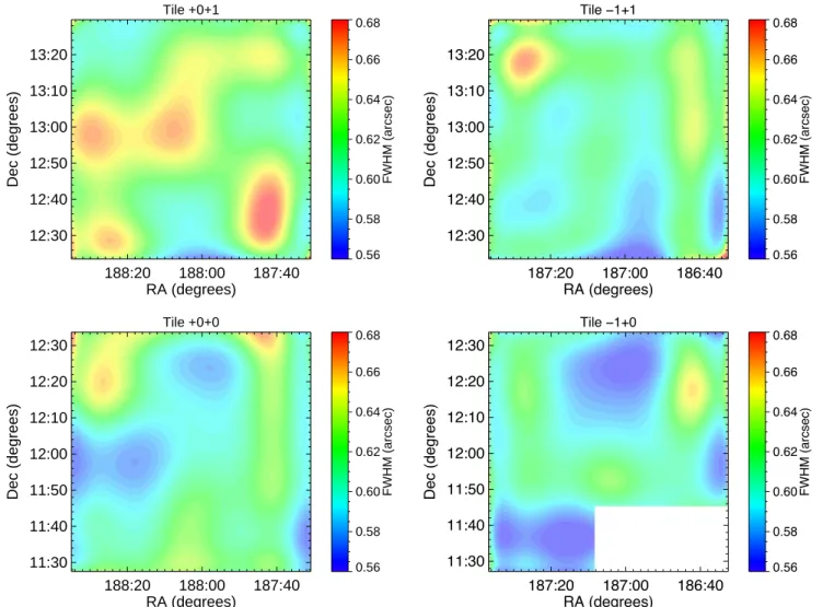
(13) NGVS-IR, I. A New Near-UV/Optical/Near-IR Globular Cluster Selection Tool. 13. Tile −1+1. Tile +0+1. 0.68. 0.68. 13:20. 0.64. 13:00. 0.62. 12:50 0.60. 0.66. 13:10. 0.64. 13:00. 0.62. 12:50 0.60. 12:40. 12:40. 0.58. 0.58. 12:30. 12:30. 0.56. 0.56. 187:20 187:00 RA (degrees). 187:40. Tile −1+0. Tile +0+0 0.68. 12:30. 0.68. 12:30. 0.66. 0.66. Dec (degrees). 12:20 12:10. 0.64. 12:00. 0.62. 11:50. 0.60. 0.58. 11:40. 0.58. 0.56. 11:30. 12:10. 0.64. 12:00. 0.62. 11:50. 0.60. 11:40 11:30. FWHM (arcsec). 12:20. 188:20 188:00 RA (degrees). 186:40. FWHM (arcsec). 188:20 188:00 RA (degrees). Dec (degrees). FWHM (arcsec). 13:10. Dec (degrees). 0.66 FWHM (arcsec). Dec (degrees). 13:20. 0.56. 187:20 187:00 RA (degrees). 187:40. 186:40. F IG . 8.— Image quality maps for the NGVS-IR pilot field split into the four quadrants corresponding to the NGVS MegaCam tile (0, 0), (+1, 0), (+1, +1), and (0, +1) (see Ferrarese et al. 2012, for details). The color bar parameterizes the full-width at half maximum (FWHM) of point-like sources in units of arc seconds over the survey area, the maximum variation of which is ∼ 20% which is mainly due to the seeing distributions of observations in each tile of the NGVS-IR mosaic as illustrated in Figure 6. 0.3. 0.3. 0.4. 0.4 0.2. 0.2. 0.1. −0.2. 0.0. 0.1. (H−K)UKIDSS. 0.0. K NGVSIR−K UKIDSS. 0.2 (H−K)2MASS. K NGVSIR−K 2MASS. 0.2. −0.2 0.0. −0.4. 0.0 −0.4. −0.1 14. 15 K2MASS (Vega). 16. −0.1 14. 15. 16. 17. 18. 19. KUKIDSS (Vega). F IG . 9.— The photometric calibration accuracy of the NGVS-IR pilot field data vs. 2MASS (left) and UKIDSS data (right). Objects in this plot are point sources according to their Ks -band morphology and NGVS/NGVS-IR colors and match coordinates in UKIDSS or 2MASS data to better than 100 . The right-hand side color bar encodes the H−K color measured in the corresponding comparison system and illustrates significant residual color terms in the photometric calibration. To avoid conversion of UKIDSS and 2MASS magnitudes into the AB system, the plots show point source magnitudes in the Vega magnitude system. Note the significantly different photometric depth (i.e. ∼ 3 mag) between the 2MASS and UKIDSS data. The data distributions in both panels are entirely dominated by the photometric uncertainties of the 2MASS and UKIDSS data.. shallowest regions in the pilot field. The 90% completeness magnitude for point-source detections and the corresponding 5σ limiting magnitude together with a conservative surface brightness limit estimate for the NGVS-IR quadrants are sum-. marized in Table 3. Figure 12 illustrates the variations of all the completeness magnitudes across the four quadrants. The main reason for the fluctuations visible across the field stems from the photomet-.

(14) 14. R. P. Muñoz et al. 0.4. 18.0. 0.3 0.4. 0.2 0.2. 0.0. 0.1. (H−K)UKIDSS. 16.0 −0.2. K NGVSIR,CORR−K UKIDSS. 0.0. 0.2 KNGVSIR (Vega). K NGVSIR−K UKIDSS. 17.0. −0.2. 15.0. 0.0. −0.4 −0.4 −0.6. 14.0 −0.4. −0.2. 0.0 0.2 (H−K) UKIDSS. 0.4. 0.6. 0.8. −0.1 14. 15. 16. 17. 18. 19. KUKIDSS (Vega). Koutput − Kinput. F IG . 10.— (Left panel): Color term resulting from the differences between the UKIDSS and WIRCam Ks filters. The shown stellar sample is the same as shown in the right panel of Figure 9. WIRCam Ks aperture photometry (in Vega mag) is used for color coding, and the best linear fit is indicated by the solid line. (Right panel): Same as right panel of Figure 9, but after applying the color-term correction to the Ks NGVS-IR data. The symbols color is parametrized according to the (H −K)UKIDSS color as indicated by the color scale next to the panel. 0.4 0.2 0.0 −0.2 −0.4 20. 21. 22. 23. 24. 1.0. Completeness. 0.8 0.6 +0+0 −1+0 +0+1 +1+1 Shallowest Deepest. 0.4 0.2. All. 0.0. 20. 21. 22 Kinput (AB). 23. 24. F IG . 11.— (Top panel): Internal photometric errors for tile +0+0 of the NGVS-IR. The errors were computed by adding artificial stars to the stacked image and then running SE XTRACTOR to do the photometry. (Bottom panel): Photometric completeness curves for the four quadrants of the NGVS-IR Pilot program region, plus the deepest and shallowest regions in the survey. The horizontal dashed lines correspond to the 90% and 50% completeness.. TABLE 3 C OMPLETENESS MAGNITUDE OF THE NGVS-IR STACKS Tile KAB,90% KAB,5σ µKs ,AB,5σ +0 + 0 23.70 24.64 25.11 −1 + 0 23.51 24.61 25.08 +0 + 1 23.32 24.16 24.63 +1 + 1 23.34 24.23 24.70 N OTE. — The 5σ limiting magnitude is measured inside a circular aperture with 0.700 radius and marks the limiting surface brightness estimate.. ric quality, i.e. FWHM distribution (see Figure 6) in each individual WIRCam tile contributing to the final quadrant stack. 6. DISCUSSION 6.1. Color-Color Diagrams. Adding more filters and a successively wider SED coverage to the investigation of astronomical objects adds more diagnostic power to the analysis and delivers ultimately more robust and astrophysically meaningful results (e.g. Park & Choi. 2005; Puzia et al. 2007). Color-color planes are efficient tools for the classification of sources in large-scale imaging surveys (e.g. Daddi et al. 2004; Faber et al. 2007). By combining near-UV and optical data from NGVS and near-IR photometry from the NGVS-IR, the advantage of spanning the entire spectral range of stellar emission from the atmospheric UV cutoff at ∼ 3200 Å to the near-infrared at ∼ 2.5 µm becomes clear when one is confronted with the vastly improved system throughputs and SED coverage of the combined NGVS+NGVS-IR filter set as illustrated in Figure 13. To construct a first NGVS+NGVS-IR source catalog, we cross-matched the NGVS-IR catalog positions with those of the NGVS u∗ griz catalog, which contains approximately half a million objects. The distribution of angular separations between Ks and i-band coordinates peaks at 0.0900 , and 95% of the detected sources (of small angular size) have a separation smaller than 0.300 . This small bias is due to the marginally resolved nature of background galaxies which constitute a large fraction of the matched catalog and introduce a random offset in the matching accuracy that appears as a systematic in one radial dimension. Future dedicated versions of those matched catalogs will be built with object-dependent procedures that allow for self-consistent optical and near-IR measurements, in particular for extended sources. However, independent measurements and subsequent matching are fully sufficient for the qualitative purposes of this paper. Historically, the optical/near-IR color-color plane that is most widely used in conjunction with large extragalactic surveys is the BzK diagram which combines (B−z) and (z−K) color indices or equivalents thereof. The diagram was highlighted by Daddi et al. (2004) as a means of identifying both passively evolving and star-forming galaxies located at redshifts larger than 1.4 or so. It was published later for a variety of deep fields, confirming the original segregation between low and high-redshift sources (e.g. Lane et al. 2007; McCracken et al. 2010, 2012; Bielby et al. 2012). The BzK technique is now being frequently used for studies of the clustering properties, intrinsic morphologies, stellar populations, and the X-ray luminosities of BzK-selected galaxies (e.g. Lin et al. 2012; Yuma et al. 2011, 2012; Ly et al. 2012; Rangel et al. 2013). Ultra-deep follow-up spectroscopy campaigns confirm the efficient selection of this type of high-redshift, starforming galaxies that suffers ∼ 10% contamination by other sources (Kurk et al. 2013)..

(15) NGVS-IR, I. A New Near-UV/Optical/Near-IR Globular Cluster Selection Tool Tile −1+1 24.2. 23.8. 13:00 12:50. 23.4. Dec (degrees). 13:10. 13:10 23.8. 13:00 12:50. 23.4. 12:40. 12:40 23.0. 12:30. 24.2. 13:20 50% completeness. 23.0. 12:30 187:20 187:00 RA (degrees). 187:40. 186:40. Tile −1+0. Tile +0+0. 12:30. 12:30. 24.2. 24.2. 12:20 23.8. 12:00 23.4. 11:50. Dec (degrees). 12:10. 50% completeness. Dec (degrees). 12:20. 12:10. 23.8. 12:00 23.4. 11:50. 50% completeness. Dec (degrees). 13:20. 50% completeness. Tile +0+1. 188:20 188:00 RA (degrees). 15. 11:40. 11:40. 23.0. 23.0. 11:30. 11:30 188:20 188:00 RA (degrees). 187:40. 187:20 187:00 RA (degrees). 186:40. F IG . 12.— Illustration of the photometric depth variations for each of the NGVS-IR pilot field quadrants. The color bar corresponds to the 50% completeness magnitude of point-like source detections. The structures in each field are mainly due to the seeing distribution of the corresponding tiles and their overlap regions.. 6.2. The NGVS+NGVS-IR analog of BzK: the gzKs. color-color plane In terms of SED coverage of the involved filters, the closest analog to the BzK diagram that can be constructed from our combined NGVS+NGVS-IR data is the gzKs diagram which is shown in the top panel of Figure 14, which illustrates our pilot field sample greyscale-coded by the Gaussian propagated total error of each contributing filter (see also Figure 13 for a comparison of the corresponding gzKs vs. BzK system throughput curves). The mean foreground extinction towards M87 is A(g) ' 0.076, A(z) ' 0.029, and A(Ks ) ' 0.007 mag, and was taken from Schlafly & Finkbeiner (2011)8 . The following analysis includes the corresponding extinction correction terms. We observe various characteristic object overdensities and sequences in the gzKs plane, such as the narrow sequence of foreground Galactic stars and other less constrained object distributions including actively star-forming and passively evolving galaxies at various redshifts that were discussed in previous works (e.g. Bielby et al. 2012; Merson et al. 2013). We use equations (1)–(8) provided in Bielby et al. (2012) to transform the BzK object selections into our gzKs color-color plane. In particular, we use the median color 8 See Appendix B for a discussion on the small color dependence of the extinction coefficients.. (u−g) = −0.194 mag of our entire sample and obtain for the selection of star-forming galaxies at z & 1.4 the following relation (shown as solid magenta line in Figure 14): (z−Ks )0 > 1.233 × (g−z)0 − 0.017.. (3). To select passively evolving galaxies at z & 1.4 we obtain (illustrated as dashed magenta line in Figure 14): (z−Ks )0 < 1.233 × (g−z)0 − 0.017 ∩ (z−Ks )0 > 2.5. (4) To select foreground stars and separate them from galaxies our transformations yield (dotted magenta line in Figure 14): (z−Ks )0 < 0.37 × (g−z)0 + 0.474. (5). The corresponding relations shown in the top panel of Figure 14 illustrate the quality of separating the classically defined BzK galaxies at z > 1.4 from the general locus of more nearby galaxies and the stellar sequence. However, it is quite evident that even with the NGVS+NGVS-IR highquality data, a clear separation of stellar foreground from the background galaxy population is not entirely possible based on the gzKs color-color diagram alone. Overall the gzKs color-color plane is the tool of choice for the study of the redshifted universe beyond Virgo due to the superior photometric depth of the g filter compared with the u∗ band observations. However, unlike any other deep optical/near-IR survey, NGVS+NGVS-IR also contains.

(16) 16. R. P. Muñoz et al.. NGVS-IR. 25000. Arbitrary Flux. System Throughput. NGVS. 0.9 0.8 VISTA/VIRCAM 0.7 CFHT/MegaCam inew 0.6 0.5 ∗ J Ks 0.4 u g r iold z 0.3 CFHT/WIRCam BzK 0.2 0.1 0.0 5000 10000 15000 20000 16 metal-poor SSP ([Fe/H]=-1.65) 14 continuously star-forming 12 e-folding SFR (tau=3 Gyr) 10 passively evolving since z=3 8 6 SEDs @z=1.4 4 2 0 5000 10000 15000 20000 ◦. λ [A]. 25000. F IG . 13.— Top panel: Direct comparison of system throughput curves, including detector efficiency, effects of telescope optics, and atmospheric absorption for all NGVS+NGVS-IR filters. Note that the NGVS-IR Ks -band filter mainly differs in detector efficiency and optics between the two instruments, i.e. CFHT/WIRCam vs. VISTA/VIRCAM. For comparison purposes, we plot the BzK system throughput curves that were used in Daddi et al. (2004) in light grey shading. Note that the atmospheric absorption effects impacting the Ks -band curve in the BzK system are not included. Bottom panel: Comparison of four different SED types: 12 Gyr old metal-poor SSP with [Fe/H]= −1.65 dex, constant SFR, e-folding SFR with τ = 3 Gyr, and passively evolving starburst since z = 3, taken from P ÉGASE (Fioc & Rocca-Volmerange 1997). Note that for SSPs with higher [Fe/H] the metal-poor SSP approximates the passively evolving starburst SED, that has been calculated for solar chemical composition. For easy comparison all SED curves at z = 0 were normalized to the flux at 2.2 µm, roughly corresponding to the effective wavelength of the Ks band. The open SED curves correspond to the same four SED types as they would appear at z = 1.4.. a nearby structure: Virgo itself. The most striking difference between our color-color diagrams and those of other surveys is not due to Virgo galaxies – these occur in negligible numbers in any given part of the diagram –, but due to GCs that are concentrated around the massive elliptical galaxy NGC 4486 (M87) and other giant ellipticals located in the central regions of Virgo (see Figure 3). To demonstrate the locus of gzKs colors of Virgo GCs we highlight radial-velocity confirmed GCs in Figure 14 as red dots (E. Peng et al., in preparation). This GC locus overlaps with the colors of stars at the blue end, and is heavily contaminated by background galaxies towards redder colors, in the gzKs diagram.. uiKs color-color plane. The stellar sequence seen in the uiKs diagram remains very clearly identified in this new plane and appears more separated from the main cloud of galaxies. This will be particularly useful for the analysis of stellar age and metallicity distribution functions in the Virgo overdensity described in Ferrarese et al. (2012). Several new narrowly defined features in the uiKs plane become visible at intermediate colors that we attempt to classify qualitatively in the following. Most importantly, however, we note that the contamination of the GC locus is very significantly reduced with the use of the uiKs filter combination. 6.3.1. An Efficient Tool for Star Cluster Selection. 6.3. The uiKs Color-Color Plane. For a photometry-based selection of GCs and other compact stellar systems, such as UCDs and dwarf galaxies, we show in the following that the most powerful color combination is given by the uiKs diagram, which combines high-quality near-UV, optical, and near-IR photometry from NGVS and NGVS-IR. The bottom panel of Figure 14 shows the uiKs color-color diagram, in which the data is deredden with the values extracted from the Schlafly & Finkbeiner (2011) maps using A(u) ' 0.097, A(i) ' 0.039, and A(Ks ) ' 0.007 mag. The typical structures seen in the gzKs diagram (top panel of Figure 14) that were classified in previous deep-field surveys appear much more prominent and better defined in the. In order to better understand the various features in the uiKs plane, we overplot in Figure 15 predictions of simple stellar population (SSP) model calculations based on a customized version of the population synthesis code P ÉGASE (Fioc & Rocca-Volmerange 1997) that includes the exactly matched throughput functions for all NGVS+NGVS-IR filters. While in the gzKs plot these SSP models coincide with the overlap region between stars and galaxies, in the uiKs plane they fall right on top of a sharply defined sequence which we identify as GCs. We note that the metallicity and age coverage of the shown SSP model predictions, i.e. Z = 0.0004, 0.001, 0.004, 0.02 and t = 8 to 13 Gyr (each running from bluer to redder colors), agrees fairly well with the GC.

(17) NGVS-IR, I. A New Near-UV/Optical/Near-IR Globular Cluster Selection Tool. 17. F IG . 14.— Illustration of the gzKs (top panel) and uiK (bottom panel) color-color diagrams of all the objects in the NGVS pilot field (grayscale dots). The symbol shading is parametrized by the total photometric error of each filter contributing to each color plane. All magnitudes are in the AB system and include the reddening corrections from Schlafly & Finkbeiner (2011). The red dots mark spectroscopically confirmed globular clusters with the systemic velocity of Virgo cluster galaxies (see text for details). The magenta solid line shows the criteria defined by Daddi et al. (2004) to isolate z > 1.4 star-forming galaxies, the dashed line to separate z > 1.4 passively evolving galaxies from nearby systems, and the dotted line to separate foreground stars from galaxies. The corresponding BzK areas are labeled accordingly in the top panel. We indicate in the bottom panel characteristic object sequences (i.e. stars, GCs, and passively evolving galaxies) and other overdensities (locations of normal and star-forming background galaxies) that are discussed in section 6.3..