Graphene transparency in weak magnetic fields
12
0
0
Texto completo
(2) Journal of Physics A: Mathematical and Theoretical J. Phys. A: Math. Theor. 48 (2015) 065402 (11pp). doi:10.1088/1751-8113/48/6/065402. Graphene transparency in weak magnetic fields David Valenzuela1, Saúl Hernández-Ortiz2, Marcelo Loewe1,3 and Alfredo Raya1,2,4 1. Instituto de Física, Pontificia Universidad Católica de Chile, Casilla 306, Santiago 22, Chile 2 Instituto de Física y Matemáticas, Universidad Michoacana de San Nicolás de Hidalgo, Edificio C-3, Ciudad Universitaria, 58040 Morelia, Michoacán, Mexico 3 Centre for Theoretical and Mathematical Physics and Department of Physics, University of Cape Town, Rondebosch 7700, South Africa E-mail: [email protected], [email protected], mloewe@fis.puc.cl and raya@ifm. umich.mx Received 27 October 2014, revised 22 December 2014 Accepted for publication 24 December 2014 Published 23 January 2015 Abstract. We carry out an explicit calculation of the vacuum polarization tensor for an effective low-energy model of monolayer graphene in the presence of a weak magnetic field of intensity B perpendicularly aligned to the membrane. By expanding the quasiparticle propagator in the Schwinger proper time representation up to order (eB)2, where e is the unit charge, we find an explicitly transverse tensor, consistent with gauge invariance. Furthermore, assuming that graphene is irradiated with monochromatic light of frequency ω along the external field direction, from the modified Maxwell equations we derive the intensity of transmitted light. Corrections to this quantity, both calculated and measured, are of the order of (eB)2/ω4. Our findings generalize and complement previously known results reported in the literature regarding the light absorption problem in graphene from the experimental and theoretical points of view, with and without external magnetic fields. Keywords: graphene, magnetic fields, vacuum polarization (Some figures may appear in colour only in the online journal). 4. Author to whom any correspondence should be addressed.. 1751-8113/15/065402+11$33.00 © 2015 IOP Publishing Ltd Printed in the UK. 1.
(3) D Valenzuela et al. J. Phys. A: Math. Theor. 48 (2015) 065402. 1. Introduction A decade has gone by since the groundbreaking experiments performed by Andrei Geim and Konstantin Novoselov [1] (Nobel Laureates in Physics in 2010) to isolate single layer membranes of graphite, graphene. Soon afterwards, theoretical [2] and experimental [3] groups highlighted the properties of charge carriers in this material, which strongly resemble ultrarelativistic electrons, thus establishing a bridge between solid state and particle physics (see, for instance, [4, 5]). Graphene has given rise to the new era of Dirac materials, with potential applications in nanotechnology, but also offering an opportunity to test the core of fundamental physics in a condensed matter environment. Mechanical, thermal and electronic properties of this two-dimensional crystal locate it among the best candidates to replace silicon in nanotechnological devices, basically due to its hardness, yet flexibility, high electron mobility and thermal conductivity [6]. The crystal structure of graphene consists of a honeycomb array of tightly packed carbon atoms, thus allowing an accurate tight-binding description. At low energies, such a description becomes in the continuous limit the Lagrangian of massless quantum electrodynamics in (2 + 1) dimensions, QED3, for the charge carriers restricted to move along the membrane [4], but in which the ‘photon’ is allowed to move throughout space in such a way that the static Coulomb interaction is still described by a potential that varies as the inverse of the distance on the plane of motion of electrons. In this form, the low-energy dynamics of graphene is in accordance with the spirit of brane-world scenarios of fundamental interactions (see, for instance, [7]), where the gauge field (photon) is allowed to move throughout the bulk (full space), but matter fields are restricted to a brane (the graphene layer). As expected, quantum field theoretical methods have been developed to describe phenomena in graphene which have been theorized in the high energy physics realm, but that would appear enhanced in this material due to the ratio of the speed of light in vacuum and the Fermi velocity of its charge carriers, c vF ≃ 300. Theoretical objects such as the effective action in external electromagnetic fields have been calculated by several authors in connection with the Schwinger mechanism for pair production and the issue of minimal conductivity [8], ideas that have been generalized to the multilayer case [9]. Other ‘relativistic’ effects discussed in the literature include the Klein paradox [10], Casimir effect [11] and dynamical formation of a mass gap from excitonic condensates [12]. Graphene properties have been handled also from the perspective of non-commutative quantum mechanics [13]. A remarkable feature of graphene is the visual transparency of the membranes. Its opacity has been measured [14] to be roughly 2.3%, with almost negligible reflectance. This observation has opened the possibility of using single layers of this crystal in combination with biomaterials to produce clean hydrogen by photocatalysis [15] with visible light. The problem of light absorption in graphene can be addressed with quantum field theoretical methods [16]. Several authors have considered the Dirac picture for its charge carriers in terms of the degrees of freedom of QED3 under different assumptions. Parity violating effects were considered in [17], whereas the influence of a strong magnetic field was considered in [18] in connection with the Faraday effect. Measurements of magneto-optical properties of epitaxial graphene have been reported in [19], in particular the polarization rotation and light absorption. Quantum Faraday and Kerr rotations have also been experimentally determined [20], and a full framework based on the equations of motion was presented in [21] to describe such effects. All the above mentioned results seem to be in accordance with the ‘relativistic’ behavior of charge carriers for a range of values of the external magnetic field intensity between 0.5 and 7 T [18]. For discussion of these results, the structure of the vacuum polarization tensor is the cornerstone. This operator has been calculated by several authors in 2.
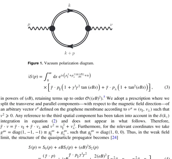
(4) D Valenzuela et al. J. Phys. A: Math. Theor. 48 (2015) 065402. the presence of a strong magnetic field perpendicularly aligned with the graphene membrane [22]. In this work, we continue the discussion, but in our considerations the external magnetic field is weak in intensity. The article is organized as follows. We start modeling the lowenergy behavior of graphene from the massless QED3 subjected to an external magnetic field perpendicular to the membrane; namely, we consider the full space, but restrict the dynamics of charge carriers in graphene to an infinite plane where the third spatial component is set to zero. Expanding the quasiparticle propagator in the weak field regime, we calculate the vacuum polarization tensor to the leading order in the external field intensity in section 2. In section 3, we introduce the polarization operator in the modified Maxwell equation to describe the propagation of electromagnetic waves in space. From the matching conditions we calculate the transmission coefficient, and from there the intensity of transmitted light. We discuss our findings and conclude in section 4. Some details of the calculation of the polarization tensor are presented in an appendix. 2. A continuous model for graphene The tight-binding approach to the description of monolayer graphene corresponds in the continuum to a massless version of quantum electrodynamics in (2 + 1) dimensions, but with a static Coulomb interaction which varies as the inverse of the distance, just as in ordinary space [4]. We adopt the conventions of [16–18] and consider an infinite graphene membrane immersed in a (3 + 1)-dimensional space oriented along the plane z = 0. The action for this model is expressed as. S=−. 1 4. ∫ d4xFμν2ˆ ˆ + ∫ d3xψ¯ D ψ ,. (1). μ with Fμν ˆ ˆ = ∂ μˆ A νˆ − ∂ νˆ A μˆ and D = iγ˜ (∂μ + ieA μ ). In our considerations, circumflexed Greek indices αˆ, βˆ , γˆ and so on take the values 0, 1, 2, 3; Greek indices μ, ν, γ, etcetera run from 0 to 2; and Latin indices a, b and so on—which label the spatial coordinates on the graphene layer—take the values 1 and 2. Moreover, the re-scaled Dirac matrices are such that γ˜ 0 = γ 0 , γ˜1,2 = vF γ1,2 , and for later convenience we also consider the matrix γ˜ 3 = γ 3, where vF is the Fermi velocity of quasiparticles in the crystal. In the natural units of the system (namely, when vF = 1), the form of the action has been dubbed reduced QED and has been proposed in the context of brane-world scenarios [7]. Measuring the response of graphene to external electromagnetic fields amounts to calculating the effective action, which in turn is expressed through the vacuum polarization ˆˆ tensor Π μν . Because in this case the dynamics of fermions is restricted to a plane, according to figure 1 we can express. ⎡ ˆ ˆ (p) = ie2 Tr ⎢ Π μν ⎣. 3. ∞. ⎤. ∫−∞ dk z δ ( k z ) ∫ (2dπk)3 γ˜ μˆS (k ) γ˜ νˆS (k + p) ⎥⎦ ,. (2). where the trace is over full space and then we set Π μˆ3 = Π 3μˆ = 0. Here, S(p) represents the quasiparticle propagator (electric charge −e) and the double fermion line in the diagram specifies that the propagator is corrected by some classical external field. We consider the situation in which a uniform magnetic field is aligned perpendicularly to the graphene membrane. We think of this field as being weak in intensity. An estimate of the strength of such fields (see below) is of the order of millitesla. We expand the Schwinger propagator in the proper time representation [23], 3.
(5) D Valenzuela et al. J. Phys. A: Math. Theor. 48 (2015) 065402. Figure 1. Vacuum polarization diagram. ∞. iS (p) =. ∫0. ds e is ( p∥ + p⊥ 2. 2 tan (eBs) eBs + iϵ. ). × ⎡⎣ γ˜ · p∥ 1 + γ 1γ 2 tan (eBs) + γ˜ · p⊥ 1 + tan2 (eBs) ⎤⎦ ,. (. ). (. ). (3). in powers of (eB), retaining terms up to order ((eB)2 ).5 We adopt a prescription where we split the transverse and parallel components—with respect to the magnetic field direction—of an arbitrary vector vμ defined on the graphene membrane according to v μ = (v∥ , v⊥ ) such that v 2 ⩾ 0 . Any reference to the third spatial component has been taken into account in the δ (k z ) integration in equation (2) and does not appear in what follows. Therefore, γ˜ · v = γ˜ · v∥ + γ˜ · v⊥ and v 2 = v∥2 + v⊥2 . Furthermore, for the relevant coordinates we take g μν = diag(1, −1, −1) ≡ g∥μν + g⊥μν , such that g∥μν = diag(1, 0, 0). Thus, in the weak field limit, the structure of the quasiparticle propagator becomes [24]. S (p) = S0 (p) + eBS1 (p) + (eB)2S2 (p) ≡. ( γ˜ · p) p2. + ieB. γ˜ · p∥ γ 1γ 2 2 2. (p ). +. 2(eB)2 ⎡ 2 2 ⎤ ⎣ p⊥ γ˜ · p∥ − p∥ γ˜ · p⊥ ⎦ . 2 4 p. ( ). (4). Here, the matrices γ1 and γ2 do not appear rescaled because the operators ± = (I ± γ1γ 2 ) 2, with I the identity matrix, correspond to the (pseudo)spin projection operators [24]. With the above expansion (4), it is straightforward to verify that the structure of the vacuum polarization is. ⎤ νˆ ˆˆ ˆˆ 2 ¯ αβ ˆ ˆ (p) = η μˆ ⎡ Π ¯ αβ Π μν αˆ ⎣ (0) (p) + (eB) Π(2) (p) ⎦ η βˆ ,. (5) ˆ. ˆ. ˆ ˆ αβ αβ where we have defined ηαˆμˆ = diag(1, vF , vF , 1). Notice that the tensors Π¯ (0) and Π¯ (2) have the block matrix structure. Π¯ =. ( ). Π 0 , 0 0. (6). where Π represent 3 × 3 matrices corresponding to the dynamical coordinates of the αβ αβ quasiparticles. Explicitly, Π(0) represents the polarization tensor in vacuum and Π(2) stands for the quadratic order contribution to the polarization tensor. The linear correction in (eB), 5. We emphasize that the Schwinger phase that accompanies the fermion propagator (3) in the proper time representation does not contribute to the vacuum polarization tensor, and thus we neglect it from the start. 4.
(6) D Valenzuela et al. J. Phys. A: Math. Theor. 48 (2015) 065402. αβ Π(1) ∼. ∫ +. d3k (2π )3. ∫. ⎡ ⎤ Tr ⎢⎣ γ˜ α ( γ˜ · k )γ˜ βγ 1γ 2( γ˜ · (k + p))∥ ⎥⎦ k 2⎡⎣ (k + p)2⎤⎦. 2. d3k (2π )3. ⎡ ⎤ Tr ⎣⎢ γ˜ αγ 1γ 2( γ˜ · k )∥ γ˜ β ( γ˜ · (k + p) )⎥⎦ ⎡ k 2⎤2 (k + p)2 ⎣ ⎦. ,. (7). upon taking the traces, reduces to αβ Π(1). ⎡ ⎢ ∼ ϵ αβγ ⎢ ⎢⎣. ∫. d3k k γ (k + p)∥ − (2π )3 k 2⎡ (k + p)2⎤2 ⎣ ⎦. ∫. ⎤ d3k k∥ (k + p) γ ⎥ ⎥. (2π )3 ⎡ k 2⎤2 (k + p)2 ⎥ ⎣ ⎦ ⎦. (8). Using the identity. Γ (p + q ) 1 = q Γ (p) Γ (q) A B p. ∫0. 1. dx. x p − 1(1 − x )q − 1 , [Ax + B (1 − x )] p + 1. (9). followed by the change of variables k → k − px , it is straightforward to show that both the integrals in the squared bracket become identical and thus the correction of order (eB) vanishes, a consequence of our working assumption that parity is preserved. In other words, contributions to the polarization arising from a Chern–Simons term are not considered in this article. αβ The magnetic field independent vacuum polarization tensor Π(0) has been calculated by many authors [16, 25]. It is of the form. ⎛ p˜ α p˜ β ⎞ αβ Π(0) = 4παΠ ⎟, ˜ vac (p) ⎜ g αβ − p˜ 2 ⎠ ⎝. (10). with α˜ = α vF2 and α = e2 (4π ) as usual. Moreover, p̃ is the magnitude of the momentum vector with components p˜ μˆ = ηνˆμˆ p νˆ , with the third spatial component set to zero, and the polarization scalar. i p˜ . 8 This vacuum contribution is transverse, as demanded by gauge invariance. On the other hand, the quadratic correction has two contributions, Πvac (p) =. (11). αβ αβ αβ = Π(2) Π(2) −11 + 2Π(2) −20. =. ∫. d3k Tr ⎡⎣ γ˜ αS1 (k ) γ˜ βS1 (k + p) ⎤⎦ (2π )3. +2. ∫. d3k Tr ⎡⎣ γ˜ αS2 (k ) γ˜ βS0 (k + p) ⎤⎦ , (2π )3. (12). αβ with a suggestive notation that the Π(2) −11 contribution comes from each of the quasiparticle αβ propagators being dressed at the first order in the external field, whereas Π(2) −20 has one 2 propagator without field, whereas the second one is dressed at order (eB) . The factor of 2 is a symmetry factor. Evaluation of these integrals is cumbersome, but straightforward. Our procedure was the following: we started by inserting the expansion in equation (4) into each of the contributions to the polarization tensor in equation (12). Then, with the aid of the 5.
(7) D Valenzuela et al. J. Phys. A: Math. Theor. 48 (2015) 065402. identity in equation (9), followed by the shift of variables k → k − p (1 − x ), after taking the traces over full space and performing the remaining contractions, we obtain. 3iα˜ αβ ⎡ 11 22 g ⎣ I104 ( p˜ ) − p˜∥2 I004 ( p˜ ) ⎤⎦, π3 4iα˜ ⎡ αβ αβ 03 23 g∥ − g⊥αβ I115 Π(2) ( p˜ ) + p˜⊥2 I105 ( p˜ ) −20 = 3 ⎣ π αβ Π(2) −11 =. ( (I. )(. 03 115. + g∥αβ. 23 ( p˜ ) + p∥2 I015 ( p˜ ) ). (. − p˜∥α p˜ β + p˜∥β p˜ α − p˜∥2 g αβ. (. + p˜⊥α p˜ β + p˜⊥β p˜ α − p˜⊥2 g αβ +. ( p˜. α β ⊥ p˜∥. ). + p˜∥α p˜⊥β. )( I. 23 015. )( I )( I. 14 015. 23 ( p˜ ) + p˜⊥2 I005 ( p˜ ) ). 14 105. 23 ( p˜ ) + p˜∥2 I005 ( p˜ ) ). 23 ( p˜ ) − 2I105 ( p˜ ) ) ⎤⎦,. (13). where the master integral fg Imnr. 1. ( p˜ ) = ∫0. f. x (1 − x ). = (−1) m+ n − r. g. ∫d. 3. k. 2 m 0. ⎡ k 2 + p˜ 2 x (1 − x ) ⎤r ⎣ ⎦. iπ r −m−n−3 2 p2. ( ). 2 n ⊥. (k ) (k ). ,. B (n + 1, r − n − 1). ˜. ⎛ 1 3⎞ × B⎜m + , r − m − n − ⎟ ⎝ 2 2⎠ ⎛ 5 5⎞ × B ⎜ f − r − m − n + , g − r − m − n + ⎟, ⎝ 2 2⎠. (14). is written in terms of beta functions B (x, y ) and whose explicit evaluation is presented in the appendix. Making use of the master integral, the quadratic correction in the external field to the polarization tensor can be written as αβ Π(2) = Π0 ( p˜ ) αβ + Π⊥ ( p˜ ) ⊥αβ ,. (15). with the transverse tensors. ⎛ p˜ α p˜ β ⎞ αβ = ⎜ g αβ − ⎟, p˜ 2 ⎠ ⎝. ⎛ p˜ α p˜ β ⎞ ⊥αβ = ⎜⎜ g⊥αβ − ⊥ 2⊥ ⎟⎟ , p˜⊥ ⎠ ⎝. (16). and the polarization scalars. ⎛ p˜∥2 ⎞ i ⎜ Π0 ( p˜ ) = 1 − 5 ⎟⎟ , p˜ 2 ⎠ 8p˜ 3 ⎜⎝. ⎛ p˜∥2 ⎞ i ⎜ ⎟. Π⊥ ( p˜ ) = 1− p˜ 2 ⎟⎠ 4p˜ 3 ⎜⎝. (17). Thus, the final expression for Παβ becomes. Π αβ (p) = 4πα˜ ⎡⎣ Πvac ( p˜ ) + (eB)2Π0 ( p˜ ) αβ + (eB)2Π⊥ ( p˜ ) ⊥αβ ⎤⎦ .. (. ). (18). The above result, equation (18), substituted back into equations (5) and (6) comprises the main result of this section and is the basis for our discussion below. Before proceeding, a few comments are in order. 6.
(8) D Valenzuela et al. J. Phys. A: Math. Theor. 48 (2015) 065402. ˆˆ • Π μν is a transverse tensor order by order in (eB). This fact justifies that our procedure to include the influence of the external magnetic field by means of expansion of the proper time representation of the quasiparticle propagator preserves gauge invariance. • Our procedure is an alternative to the traditional approach, in which the vacuum polarization tensor is expressed as a double proper time integral [23, 26–28]. In fact, for the particular case of QED in (2 + 1) dimensions considered in [28], the weak field expansion of the polarization scalars, equations (48)–(50) of that reference, match our findings in the massless limit, when we set vF = 1. ˆˆ We shall use the expressions for Π μν developed in this section to discuss the problem of light absorption in graphene.. 3. Light absorption From the action of our model, equation (1), we can describe the propagation of electromagnetic waves throughout space according to the modified Maxwell equations ˆ ˆA = 0, ˆ ˆ + δ (z ) Π νρ ∂ μˆF μν ρˆ. (19). which fulfill the conditions. A μˆ. ( ∂zA μˆ ) z=0. +. z=0+. − A μˆ. (. − ∂z A μˆ. z = 0−. ) z=0. −. = 0, = Πμˆνˆ Aνˆ. z = 0.. (20). Following [16–18], we interpret the delta function in equation (19) as a current along the graphene plane. Thus, from Ohm’s law,. ja = σab E b.. (21). Assuming a varying electric field with frequency ω expressed in a temporal gauge A0 = 0, namely, Eb = iωAb , and noticing, from the generalized Maxwell equations (19), that ja ≃ Πab Ab , we can identify the conductivity tensor as Πab σab = . (22) iω From the symmetric character of the polarization tensor, the transverse conductivity vanishes identically. For the problem of light absorption, let us consider a plane wave of frequency ω, which travels along the z-direction from below the graphene layer with a linear polarization along the êx direction. Moreover, considering that the wave propagates perpendicularly to the graphene plane, the reflected and transmitted waves can be described as. ⎧ eˆ e ik z z + r eˆ + r eˆ e−ik z z , z < 0 ⎪ x xx x xy y A = e−iωt ⎨ ⎪ t xx eˆx + t xy eˆy e ik z z , z>0 ⎩. (. ). (. ). (23). where êx, y are the unit vectors along the directions x and y on the membrane. Thus, from the general form of the vacuum polarization tensor, the boundary conditions (20) simplify to. Aa. z=0+. ( ∂ z Aa ) z = 0. +. − Aa. z = 0− z = 0−. − ( ∂ z Aa ). z = 0−. = 0, = αΨ (ω) δ abAb. 7. z = 0,. (24).
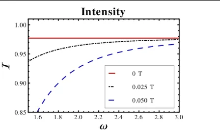
(9) D Valenzuela et al. J. Phys. A: Math. Theor. 48 (2015) 065402. Figure 2. Intensity of transmitted light as a function of the incoming electromagnetic wave frequency ω (in eV) for different values of the external magnetic field but preserving the weakness of the intensity of our approximation. The solid red curve corresponds to the vacuum case, B = 0 T; dot–dashed black curve, B = 25 mT; longdashed blue curve, B = 50 mT.. where. Ψ (ω) = α ⎡⎣ Πvac (ω) + (eB)2Π0 (ω) ⎤⎦ .. (25). Thus, the transmission coefficients can be straightforwardly obtained [16–18]. t xx =. 2ω , iαΨN (ω) + 2ω. t xy = 0,. (26). with ΨN (ω) = NΨ (ω), accounting for the degrees of freedom of charge carriers. Therefore, the intensity of transmitted light is. α Im ΨN (ω) + α2 . ω In terms of the conductivity tensor σ, can be expressed as. ( ). 2. = t xx ≃ 1 +. ( ). = 1 − Re σxx + α 2 .. (27). (28). Substituting the explicit form of the polarization scalars, we finally arrive at the main result of this article, namely,. ⎛ (eB)2 ⎞ = 1 − απ ⎜ 1 + 4 ⎟, ω4 ⎠ ⎝. (29). which is plotted in figure 2 as a function of the frequency of incident light ω for several values of the external magnetic field. To have an idea of the scales involved, for visible light, within the estimate of 85–97% of transparency of graphene samples, the magnetic field intensities are of a few millitesla. Comparing with the measured universal absorption rate ≃ απ = 2.3% [14], we conclude that, in the weak field limit, the intensity of transmitted light is corrected by factors (eB)2/ω4, in consistency with the experimental and theoretical findings for these quantities in the absence of external fields as well as in the presence of a strong magnetic field [16, 19–22]. 8.
(10) D Valenzuela et al. J. Phys. A: Math. Theor. 48 (2015) 065402. 4. Final remarks In this work, we have calculated the vacuum polarization tensor in a low energy effective model of graphene based on the massless QED3. We have considered a uniform magnetic field aligned perpendicularly to the graphene membrane and expanded the charge carrier propagator in the weak field regime. The Passarino–Veltman types of integral involved in the calculation of the polarization operator were obtained after a lengthy, but straightforward, ˆˆ procedure from a single master integral that yields a transverse Π μν , equation (18), in every order of expansion on the intensity of the external field. One part of this object is inherited from the form of the polarization tensor in vacuum and receives a leading correction of order (eB)2, whereas the second part is transverse in the coordinates on the graphene membrane and vanishes in the absence of the field. Direct calculation does not always render a manifestly transverse polarization operator [29], for instance in ordinary QED. Spurious terms might arise as a consequence of a regularization procedure. Nevertheless, careful treatment of the regulators ensures that gauge invariance is preserved for arbitrary magnetic field strength. QED3, being superrenormalizable, lacks UV-regularization issues. We have presented an alternative calculation to the standard representation of the polarization tensor as a double proper time integral [23, 26–28], which manifestly preserves gauge invariance. As an application of the vacuum polarization tensor, we have estimated the light absorption in graphene. We observe a deviation of the form (eB)2/ω4 as compared to the vacuum result for graphene opacity. Our findings are in agreement with previously reported theoretical calculations [16–18, 21] as well as the experimental light absorption of 2.3% per graphene membrane [14]. Further applications of the polarization tensor in weak magnetic fields presented here and the effective action derived from it are under scrutiny and will be presented elsewhere. Acknowledgments We acknowledge valuable discussions with Cristián Villavicencio, Ángel Sánchez and María Elena Tejeda. AR and SH-O acknowledge CONACYT (Mexico) for financial support for a sabbatical and a short visit to PUC, respectively, and CIC-UMSNH under grant No 4.22, as well as the hospitality of PUC, where the main part of this work was carried out. ML acknowledges final support from FONDECYT (Chile) grant Nos 1130056 and 1120770. DV acknowledges support from CONICYT (Chile). Appendix In this appendix, we compute the master integral in equation (14). For this purpose, we write fg Imnr =. ∫0. 1. x f (1 − x ) gJmnr (x ; p),. (A.1). with. Jmnr (x ; p) =. ∫ d3k. k∥2 m k ⊥2n ⎡ k 2 + p2 x (1 − x ) ⎤r ⎣ ⎦. .. (A.2). After Wick rotating to Euclidean space, writing d3k = π dk∥ k ⊥ dk ⊥ and with the aid of the identity 9.
(11) D Valenzuela et al. J. Phys. A: Math. Theor. 48 (2015) 065402. B (x , y ) = 2. ∫0. ∞. (. dt t 2x − 1 1 + t 2. −x − y. ). ,. (A.3). we immediately obtain. ⎛ 1 3⎞ Jmnr (x ; p) = (−1) m+ n − r iπB (n + 1, r − n − 1) B ⎜ r + , r − m − n − ⎟ ⎝ 2 2⎠ 1 × . ⎡ p2 x (1 − x ) ⎤r − m− n − 3 2 ⎣ ⎦. (A.4). Then, the remaining integral over x in equation (A.1) can be performed from the definition of the beta function. B (x , y ) =. ∫0. 1. dt t x − 1 (1 − t ) y − 1,. (A.5). which finally lead us to the result (14). References [1] [2] [3] [4] [5] [6] [7]. [8] [9] [10] [11]. [12]. [13] [14] [15] [16] [17] [18] [19] [20]. Novoselov K S et al 2005 Nature 438 197 Gusynin V P and Sharapov S G 2005 Phys. Rev. Lett. 95 146801 Zhang Y et al 2005 Nature 438 201 Gusynin V P, Sharapov S G and Carbotte J P 2007 Int. J. Mod. Phys. B 21 4611 Geim A K and Novoselov K S 2007 Nat. Mat. 6 183 Savage N 2012 Nature 438 S30 Gorbar E V, Gusynin V P and Miransky V A 2001 Phys. Rev. D 64 105028 Teber S 2012 Phys. Rev. D 86 025005 Kotikov A V and Teber S 2013 Phys. Rev. D 87 087701 Kotikov A V and Teber S 2014 Phys. Rev. D 89 065038 Teber S 2014 Phys. Rev. D 89 067702 Beneventano C G, Giaconni P, Santangelo E M and Soldati R 2007 J. Phys. A 40 F35 Katsnelson M I, Volovik G E and Zubkov M A 2013 Ann. Phys. 331 160 Katsnelson M I, Geim A K and Novoselov K S 2006 Nat. Phys. 2 620 Dobson J F, White A and Rubio A 2006 Phys. Rev. Lett. 96 073201 Bordag M, Fialkovsky I V, Gitman D M and Vassilevich D V 2009 Phys. Rev. B 80 245406 Gómez-Santos G 2009 Phys. Rev. B 80 245424 Sernelius B E 2011 Eur. Phys. Lett. 95 57003 Sarabadani J, Naji A, Asgari R and Podgornik R 2011 Phys. Rev. B 84 155407 Khsevshenko D V 2009 J. Phys:. Condens. Matter 21 075303 Sabio J, Sols F y and Guinea F 2010 Phys. Rev. B 82 121413 Gonzalez J 2010 Phys. Rev. B 82 155404 Gamayun O V, Gorbar E V and Gusynin V I 2010 Phys. Rev. B 81 075429 Wang J-R and Lui G Z 2011 J. Phys.: Condens. Matter 23 155602 Wang J-R and Lui G Z 2011 J. Phys.: Condens. Matter 23 345601 Falomir H, Gamboa J, Loewe M and Nieto M 2012 J. Phys. A: Math. Theor. 45 135308 Nair R R, Blake P, Grigorenko A N, Novoselov K S, Booth T J, Stauber T, Peres N M R and Geim A K A K 2008 Science 320 1308 Wang P et al 2014 ACS Nano 8 7995 Fialkovsky I and Vassilevich D V 2012 Int. J. Mod. Phys. A 27 1260007 Fialkovsky I and Vassilevich D V 2012 Int. J. Mod. Phys. Conf. Ser. 14 88–99 Fialkovsky I and Vassilevich D V 2009 J. Phys. A: Math. Theor. 42 442001 Fialkovsky I and Vassilevich D V 2012 Eur. Phys. J. B 85 384 Grassee I, Walter A L, Ostler M, Bostwick A, Seyller T, van der Marel D and Kuzmenko A B 2011 Nat. Phys. 7 48 Shimano R, Yumoto G, Yoo J Y, Matsunaga R, Tanabe S, Hibino H, Morimoto T and Aoki H 2013 Nat. Comm. 4 1841 10.
(12) D Valenzuela et al. J. Phys. A: Math. Theor. 48 (2015) 065402. [21] Ferreira A, Viana-Gomes J, Bludov Yu V, Pereira V, Peres N M R and Castro Neto A H 2011 Phys. Rev. B 84 235410 [22] Gorbar E V, Gusynin V P, Miransky V A and Shovkovy I A 2002 Phys. Rev. B 66 045108 Gusynin V P and Sharapov S G 2006 Phys. Rev. B 73 245411 Gusynin V P, Sharapov S G and Carbotte J P 2007 J. Phys.: Condens. Matter. 19 026222 Gusynin V P, Sharapov S G and Carbotte J P J P 2009 New J. Phys. 11 095013 Pyatkovskiy P K 2009 J. Phys.: Condens. Matter. 21 025506 Pyatkovskiy P K and Gusynin V P 2011 Phys. Rev. B 83 075422 [23] Schwinger J S 1951 Phys. Rev. 82 664 [24] Chyi T-K, Hwang C-W, Kao W-F, Lin G-L, Ng K-W and Tseng J-J 2000 Phys. Rev. D 62 105014 [25] Appelquist T W, Bowick M J, Karabali D and Wijewardhana L C R 1986 Phys. Rev. D 33 3704 [26] Dittrich W and Reuter M 1985 Effective Lagrangians in Quantum Electrodynamics (Berlin: Springer) Dittrich W and Gies H 2000 Probing the Quantum Vacuum (Berlin: Springer) [27] Schubert C and Varlamov V 2013 Math. Meth. Appl. Sci. 34 1638 [28] Shpagin A V 1996 Dynamical mass generation in (2+1) dimensional electrodynamics in an external magnetic field arXiv:hep-ph/9611412 [29] Chao J, Yu L and Huang M 2014 Phys. Rev. D 90 045033. 11.
(13)
Figure
Documento similar