Deep multi survey classification of variable stars

Texto completo

(1)PONTIFICIA UNIVERSIDAD CATÓLICA DE CHILE ESCUELA DE INGENIERÍA. DEEP MULTI-SURVEY CLASSIFICATION OF VARIABLE STARS. CARLOS ALFONSO AGUIRRE ORELLANA. Thesis submitted to the Office of Research and Graduate Studies in partial fulfillment of the requirements for the degree of Master of Science in Engineering. Advisor: KARIM PICHARA. Santiago de Chile, June 2018 c MMXVIII, C ARLOS A LFONSO AGUIRRE O RELLANA.

(2) PONTIFICIA UNIVERSIDAD CATÓLICA DE CHILE ESCUELA DE INGENIERÍA. DEEP MULTI-SURVEY CLASSIFICATION OF VARIABLE STARS. CARLOS ALFONSO AGUIRRE ORELLANA. Members of the Committee: KARIM PICHARA FELIPE NÚÑEZ RETAMAL JUAN CARLOS MAUREIRA GUILLERMO CABRERA VIVES RODRIGO ESCOBAR MORAGAS Thesis submitted to the Office of Research and Graduate Studies in partial fulfillment of the requirements for the degree of Master of Science in Engineering. Santiago de Chile, June 2018 c MMXVIII, C ARLOS A LFONSO AGUIRRE O RELLANA.

(3) Grateful to my family and friends, especially to my mother and father.

(4) TABLE OF CONTENTS. LIST OF TABLES. vi. LIST OF FIGURES. vii. RESUMEN. ix. ABSTRACT. x. 1.. INTRODUCTION. 1. 2.. RELATED WORK. 6. 3.. BACKGROUND THEORY. 9. 4.. 5.. 6.. 3.1.. Artificial Neural Networks . . . . . . . . . . . . . . . . . . . . . . . . . .. 9. 3.2.. Convolutional Neural Nets . . . . . . . . . . . . . . . . . . . . . . . . . .. 13. METHOD DESCRIPTION. 15. 4.1.. Pre-processing . . . . . . . . . . . . . . . . . . . . . . . . . . . . . . . .. 16. 4.2.. First Convolution . . . . . . . . . . . . . . . . . . . . . . . . . . . . . . .. 17. 4.3.. Second Convolution . . . . . . . . . . . . . . . . . . . . . . . . . . . . .. 18. 4.4.. Flatten Layer . . . . . . . . . . . . . . . . . . . . . . . . . . . . . . . . .. 19. 4.5.. Hidden Layer . . . . . . . . . . . . . . . . . . . . . . . . . . . . . . . . .. 19. 4.6.. Softmax Layer . . . . . . . . . . . . . . . . . . . . . . . . . . . . . . . .. 19. DATA. 20. 5.1.. OGLE-III . . . . . . . . . . . . . . . . . . . . . . . . . . . . . . . . . . .. 20. 5.2.. The Vista Variable in the Vı́a Láctea . . . . . . . . . . . . . . . . . . . . .. 20. 5.3.. CoRoT . . . . . . . . . . . . . . . . . . . . . . . . . . . . . . . . . . . .. 21. EXTRACTION OF DATA. 23. 6.1.. Time & Magnitude Difference . . . . . . . . . . . . . . . . . . . . . . . .. 23. 6.2.. Light Curve padding . . . . . . . . . . . . . . . . . . . . . . . . . . . . .. 23. iv.

(5) 6.3. 7.. 8.. 9.. A Light curve data augmentation model . . . . . . . . . . . . . . . . . . .. PARAMETER INITIALIZATION. 24 26. 7.1.. Parameters . . . . . . . . . . . . . . . . . . . . . . . . . . . . . . . . . .. 26. 7.2.. Layers . . . . . . . . . . . . . . . . . . . . . . . . . . . . . . . . . . . .. 26. 7.3.. Activation functions . . . . . . . . . . . . . . . . . . . . . . . . . . . . .. 27. 7.4.. Dropout . . . . . . . . . . . . . . . . . . . . . . . . . . . . . . . . . . . .. 27. RESULTS. 29. 8.1.. Computational Run Time . . . . . . . . . . . . . . . . . . . . . . . . . . .. 29. 8.2.. Results with general classes of variability. . . . . . . . . . . . . . . . . . .. 30. 8.3.. Results with subclasses of variability . . . . . . . . . . . . . . . . . . . . .. 34. CONCLUSION. 39. REFERENCES. 40. v.

(6) LIST OF TABLES. 5.1. Class distribution of OGLE-III labeled set. . . . . . . . . . . . . . . . . . . .. 21. 5.2. Class distribution of VVV labelled set. . . . . . . . . . . . . . . . . . . . . .. 22. 5.3. Class distribution of CoRoT labelled set. . . . . . . . . . . . . . . . . . . . .. 22. 7.1. Parameters used for the proposed architecture . . . . . . . . . . . . . . . . . .. 28. 8.1. Approximately time of extraction of features and training the algorithms. . . .. 30. 8.2. Accuracy per class with the total amount of stars use for each one (in parenthesis). 31. 8.3. Accuracy per subclass with the total amount of stars use for each one (in parenthesis). . . . . . . . . . . . . . . . . . . . . . . . . . . . . . . . . . . .. vi. 36.

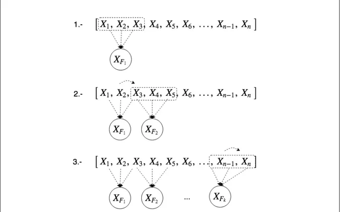
(7) LIST OF FIGURES. 1.1. Comparison of RR Lyrae ab and Cepheid stars in OGLE-III, VISTA and Corot Survey respectively. Difference between magnitude and cadence is shown. . . .. 1.2. 2. Comparison of FATS feature in RR Lyrae ab using histogram plots of stars using OGLE-III, Corot and Vista Surveys. Every feature is shown with its relative importance in classification as mention in Nun et al. 2015. . . . . . . . . . . .. 3.1. 3. The forming basic unit the perceptron. It combines the inputs with their respective weights and apply a non-linear function to produce the output. A bias b0 is added to each perceptron letting it change the starting point. . . . . . . . . . . . . . .. 3.2. A vanilla neural network with an input, hidden and output layer. Total number of hyperparameters 17. . . . . . . . . . . . . . . . . . . . . . . . . . . . . . . .. 3.3. 10. 11. Step by step of a convolution process. A sliding window and a moving step are applied to the data and given as an input to the next layer. . . . . . . . . . . . .. 13. 4.1. The Convolutional Network Architecture for multi-survey. . . . . . . . . . . .. 15. 4.2. Each light curve is transformed using a matrix with two channels, time and magnitude. For every channel, the maximum number of points is N . Each light curve is transformed using the difference between points and a new matrix is created with two channels. . . . . . . . . . . . . . . . . . . . . . . . . . . .. 6.1. Example of a new light curve using a burning parameter of 2 and a step parameter of 1. . . . . . . . . . . . . . . . . . . . . . . . . . . . . . . . . . . . . . . .. 8.1. 24. Accuracy of the training model using a 10-fold stratified cross validation with classes. . . . . . . . . . . . . . . . . . . . . . . . . . . . . . . . . . . . . .. 8.2. 17. 31. Confusion matrix per class and survey for the convolutional neural network. Empty cells correspond to 0%. . . . . . . . . . . . . . . . . . . . . . . . . . vii. 33.

(8) 8.3. Confusion matrix per class and survey using Random Forest algorithm. Empty cells correspond to 0%. . . . . . . . . . . . . . . . . . . . . . . . . . . . . .. 8.4. Accuracy of the training model using a 10-fold stratified cross validation with subclasses. . . . . . . . . . . . . . . . . . . . . . . . . . . . . . . . . . . . .. 8.5. 35. Confusion matrix per class and survey for the convolutional neural network. Empty cells correspond to 0. . . . . . . . . . . . . . . . . . . . . . . . . . .. 8.6. 34. 37. Confusion matrix per class and survey using Random Forest algorithm. Empty cells correspond to 0. . . . . . . . . . . . . . . . . . . . . . . . . . . . . . .. viii. 38.

(9) RESUMEN. Durante la última década, se ha realizado una gran cantidad de esfuerzo en clasificar estrellas variables utilizando diferentes técnicas de aprendizaje automático. Tı́picamente, las curvas de luz se representan como vectores de descriptores estadı́sticos los cuales se utilizan para entrenar distintos algoritmos. Estos descriptores demandan grandes poderes de cómputo, haciendo imposible crear formas escalables y eficientes de clasificar automáticamente estrellas variables. Además, las curvas de luz de diferentes catálogos no se pueden integrar y analizar juntas de manera inmediata. Por ejemplo, al tener variaciones en la cadencia y filtros, las distribuciones de caracterı́sticas se vuelven parciales y requieren costosos modelos de calibración de datos. La gran cantidad de datos que se generarán pronto hacen necesario desarrollar arquitecturas de aprendizaje automático escalables. Estas arquitecturas deben ser capaces de analizar curvas de luz de diferentes catálogos sin costosas técnicas de integración. Las redes neuronales convolucionales han mostrado resultados impresionantes en la clasificación y representación de imágenes. Son capaces de clasificar objetos en imágenes con altos niveles de precisión. En este trabajo, presentamos un novedoso modelo de aprendizaje profundo para la clasificación de curvas de luz, basado principalmente en unidades convolucionales. Nuestra arquitectura recibe como entrada las diferencias entre el tiempo y la magnitud de las curvas de luz. Captura los patrones de clasificación esenciales independientemente de la cadencia y el filtro, y sin la necesidad de calcular ninguna caracterı́stica estadı́stica. Probamos nuestro método usando tres catálogos diferentes: OGLE-III; Corot; y VVV, que difieren en filtros, cadencia y área del cielo. Mostramos que además del beneficio de la escalabilidad, nuestro modelo obtiene niveles de precisión comparables con el estado del arte en clasificación de estrellas variables.. Palabras Claves: curvas de luz, estrellas variables, clasificacin supervisada, redes neuronales, aprendizaje profundo. ix.

(10) ABSTRACT. During the last decade, a considerable amount of effort has been made to classify variable stars using different machine learning techniques. Typically, light curves are represented as vectors of statistical descriptors or features that are used to train various algorithms. These features demand big computational powers that can last from hours to days, making impossible to create scalable and efficient models to automatically classify variable stars. Also, light curves from different surveys cannot be integrated and analyzed together when using features, because of observational differences. For example, having variations in cadence and filters, feature distributions become biased and require expensive data-calibration models. The vast amount of data that will be generated soon make necessary to develop scalable machine learning architectures. These architectures have to be able to analyze light curves from different sources without expensive integration techniques. Convolutional Neural Networks have shown impressing results in raw image classification and representation within the machine learning literature. They can classify objects in images with high accuracy levels, even when images come from different contexts, instruments, light backgrounds, objects size, etc. In this work, we present a novel Deep Learning model for light curve classification, mainly based on convolutional units. Our architecture receives as input the differences between time and magnitude of light curves. It captures the essential classification patterns regardless of cadence and filter, and without the need of computation of any statistical feature. We tested our model using three different surveys: OGLE-III; Corot; and VVV, which differ in filters, cadence, and area of the sky. We show that besides the benefit of scalability, our model obtains state of the art levels accuracy in light curve classification benchmarks. It achieves +90% and +80% overall accuracy in most of the classes and subclasses respectively.. Keywords: light curves, variable stars, supervised classification, neural net, deep learning. x.

(11) 1. INTRODUCTION Variable stars are crucial for studying and understanding the galaxy and the universe. There has been a considerable amount of effort trying to automate the classification of variable stars [Benavente et al., 2017, Bloom & Richards, 2011, Debosscher et al., 2007, Mackenzie et al., 2016, Nun et al., 2015, Pichara et al., 2012, Pichara, Protopapas, & León, 2016, Sarro et al., 2009]. Variable stars such as RR Lyrae, Mira, and Cepheids are important for distant ladder measurements as shown in Bloom & Richards 2011. The feasibility to classify variable stars is closely related to the way light curves are represented. Light curves are discrete time series that show the intensity of light emitted by a celestial object over time. They are not uniformly sampled and depends on the particular band or filter they were observed. Moreover, the length of the light curves depends on the amount of time a variable star has been observed along with the cadence of the observations (time between measurements). One way to classify variable stars, is to create vectors of statistical descriptors, called features, to represent each light curve [Bloom & Richards, 2011, Nun et al., 2015]. One of the most popular set of statistical features is presented in Nun et al. [2015], also known as FATS features (stands for Feature Analysis for Time Series). These vectors demand large computational resources and aim to represent the most relevant characteristics of light curves. A lot of effort has been made to design these features, and the creation of new ones implies a lot of time and research. The future surveys in Astronomy make infeasible to use these features. One example of the huge amount of data is The Large Synoptic Survey Telescope (LSST) [Abell et al., 2009, Borne et al., 2007] that will start operating on 2022. It is estimated that the LSST will produce 15 to 30TB of data per night. New ways of treating this information have been proposed [Gieseke et al., 2017, Mackenzie et al., 2016, Naul et al., 2017, Valenzuela & Pichara, 2017a]. Mackenzie et al. 2016’s uses an unsupervised feature learning algorithm to classify variable stars. Valenzuela & Pichara 2017a perform unsupervised classification by extracting local patterns among light curves and create a ranking of similarity. To extract such patterns they use a sliding window as done in Mackenzie et al. 2016.. 1.

(12) Figure 1.1. Comparison of RR Lyrae ab and Cepheid stars in OGLE-III, VISTA and Corot Survey respectively. Difference between magnitude and cadence is shown.. Either way, none of these methods can be applied immediately in new surveys. The limited overlap and depth coverage among surveys makes difficult to share data. The difference in filter and cadence makes it even harder without any transformation to the data. Figure 1.1 shows an example of the complexity that exists among stars and surveys. Light curves have a difference in magnitude and time, and most of the time they are not human-eye recognizable, even by experts. Since all the magnitudes are calibrated by using statistics, it does not work correctly because of underlying differences between surveys. Figure 1.2 shows a comparison of statistical features of RR Lyrae ab stars using three different catalogs. To the best of our knowledge, little efforts have been made to create invariant training sets within the datasets. 2.

(13) Benavente et al. 2017 proposed an automatic survey invariant model of variable stars transforming FATS statistical vectors [Nun et al., 2015] from one survey to another. As previously mentioned, these features have the problem of being computationally infeasible. Therefore, there is a necessity of faster techniques able to use data from different surveys.. Figure 1.2. Comparison of FATS feature in RR Lyrae ab using histogram plots of stars using OGLE-III, Corot and Vista Surveys. Every feature is shown with its relative importance in classification as mention in Nun et al. 2015.. 3.

(14) Artificial neural networks (ANNs) have been known for decades [Cybenko, 1989, Hornik, 1991], but the vast amount of data needed to train them made them infeasible in the past. The power of current telescopes and the amount of data they generate have practically solved the problem. The improvement in technology and the big amount of data makes ANNs feasible for the future challenges in astronomy. Artificial neural networks or deep neural networks create their own representation by combining and encoding the input data using non-linear functions [LeCun et al., 2015]. Depending on the number of hidden layers, the capacity of extracting features improve, together with the need for more data [LeCun et al., 2015]. Convolutional neural networks (CNNs) are a particular type of neural network that have shown essential advantages in extracting features from images [Krizhevsky et al., 2012]. CNNs use filters and convolutions that respond to patterns of different spatial frequency, allowing the network to learn how to capture the most critical underlying patterns and beat most of the classification challenges [Krizhevsky et al., 2012]. Time series, as well as in images, have also proven to be a suitable field for CNNs [Jiang & Liang, 2016, Zheng et al., 2014]. In this document, we propose a convolutional neural network architecture that uses raw light curves from different surveys. Our model can encode light curves and classify between classes and subclasses of variability. Our approach does not calculate any of the statistical features such as the ones proposed in FATS, making our model scalable to vast amounts of data. In addition, we present a novel data augmentation schema, specific for light curves, used to balance the proportion of training data among different classes of variability. Data augmentation techniques are widely used in the image community [Dieleman et al., 2015, Gieseke et al., 2017, Krizhevsky et al., 2012]. We present an experimental analysis using three datasets: OGLE-III [Udalski, 2004], VISTA [Minniti et al., 2010] and Corot [Baglin et al., 2002, Bordé et al., 2003]. The used datasets differ in filters, cadence and observed sky-area. Our approach obtains comparative results with a Random Forest (RF) classifier, the most used model for light curve classification [Dubath et al., 2011, Gieseke et al., 2017, Long et al., 2012, Richards et al., 2011], that 4.

(15) uses statistical features. Finally, we produce a catalog of variable sources by cross-matching VISTA and OGLE-III and made it available for the community. 1. The remainder of this document is organized as follows: Chapter 2 gives an account of previous work on variable stars classification and convolutional neural networks. In Chapter 3 we introduce relevant background theory. Chapter 4 explains our architecture and Chapter 5 describes the datasets that are used in our experiments. Chapter 6 explains the modifications that are made to the data and Chapter 7 gives an account of the parameters that are used in the architecture. Chapter 8 shows our experimental analysis and Section 8.1 presents a study of the time complexity of our model. Finally, in Chapter 9, the main conclusions and future work directions are given.. 1. Datasets will be available in http://gawa.academy/profile/¡authorusername¿/. A Data Warehouse for astronomy [Machin et al., 2018]. 5.

(16) 2. RELATED WORK As mention before, there has been huge efforts to classify variable stars [Huijse et al., 2014, Mackenzie et al., 2016, Nun et al., 2014, 2015, Pichara, Protopapas, & Leon, 2016, Richards et al., 2011, Valenzuela & Pichara, 2017b]. The main approach has been the extraction of features that represent the information of light curves. Debosscher et al. 2007 was the first one to proposing 28 different features extracted from the photometric analysis. Sarro et al. 2009 continue his work by introducing the color information using the OGLE survey and carrying out an extensive error analysis. Richards et al. 2011 use 32 periodic features as well as kurtosis, skewness, standard deviation, and stetson, among others, for variable stars classification. Pichara et al. 2012 improve quasars detection by using a boosted Random Forest with continuous auto regressive features (CAR). Pichara & Protopapas 2013 introduce a probabilistic graphical model to classify variable stars by using catalogs with missing data. Kim et al. 2014 use 22 features for classifying classes and subclasses of variable stars using random forest. Nun et al. 2015 published a library that facilitates the extraction of features of light curves named FATS (Feature Analysis for Time Series). More than 65 features are compiled and put together in a Python library1. Kim & Bailer-Jones 2016 publish a library for variable stars classification among seven classes and subclasses. The library extracts sixteen features that are considered survey-invariant and uses random forest for doing the classification process. Extracting statistical vectors has been the main approach but the high computational cost and the research time needed, make it infeasible for future surveys. A novel approach that differs from most of the previous papers is proposed by Mackenzie et al. 2016. He face the light curve representation problem by designing and implementing an unsupervised feature learning algorithm. His work uses a sliding window that moves over the light curve and get most of the underlying patterns that represent every light curve. This window extracts features that are as good as traditional statistics, solving the problem of high. 1. Information about the features and manuals of how to use them are available as well.. 6.

(17) computational power and removing the human from the pre-processing loop. Mackenzie et al. 2016 work shows that automatically learning the representation of light curves is possible. Since every survey has different cadences and filters, research has been done to learn how to transfer information among them. The ability to use labeled information without an extensive work accelerates the process of bringing new labeled datasets to the community. Long et al. 2012 propose using noise and periodicity to match distributions of features between catalogs. Also, show that light curves with the same source and different surveys would normally have different values for their features. Benavente et al. 2017 represent the joint distribution of a subset of FATS features from two surveys and creates a transformation between them by using a probabilistic graphical model with approximate inference. Even though he use FATS for his experiments, they can be easily changed to Mackenzie et al. 2016 features, making the process even faster. Pichara, Protopapas, & León 2016 present a metaclassification approach for variable stars. He show an interesting framework that combines classifiers previously trained in different sets of classes and features. His approach avoids to re-train from scratch on new classification problems. The algorithm learns the meta-classifier by using features, but including their computational cost in the optimization of the model. All methods mentioned above invest lots of efforts finding a way to represent light curves. There have been several works in deep learning where the network itself is the one in charge of learning the representation of data needed for classification. Baglin et al. 2002 use a vanilla neural network for classifying microlensing light curves from other types of curves such as variable stars. Belokurov et al. 2003 continue the work presenting two neural networks for microlensing detection. Krizhevsky et al. 2012 show the importance of CNNs for image-feature-extraction, and use them to classify, achieving impressive results. Zeiler & Fergus 2014 study the importance of using filters in each convolutional layer and explain the feature extraction using the Imagenet dataset. Dieleman et al. 2015 apply galaxy morphology classification using deep convolutional neural networks. Cabrera-Vives et al. 2017 use a rotation-invariant convolutional neural network to classify transients stars in the HITS. 7.

(18) survey. Mahabal et al. 2017 transform light curves into a two-dimensional array and perform classification with a convolutional neural network. CNNs not only work on images. Many studies have been done using one-dimensional time series. Zheng et al. 2014 use them to classify patient’s heartbeat using a multi-band convolutional neural network on the electrocardiograph time series. Jiang & Liang 2016 create a decision maker for a cryptocurrency portfolio using a CNN on the daily price information of each coin.. 8.

(19) 3. BACKGROUND THEORY In this chapter, we introduce the basics on both artificial neural networks and convolutional neural networks, to gain the necessary insights on how our method works.. 3.1. Artificial Neural Networks Artificial neural networks (ANN) are computational models based on the structure and functions of biological axons [Basheer & Hajmeer, 2000]. The ability for axons to transmit, learn and forget information has been the inspiration for neural networks. ANNs are capable of extracting complex patterns from the input data using nonlinear functions and learn from a vast amount of observed data. ANNs have been used in different areas such as speech recognition [Graves et al., 2013, Xiong et al., 2016, 2017], image recognition [Krizhevsky et al., 2012, Ren et al., 2015, Szegedy et al., 2015], and language translation [Jean et al., 2014, Sutskever et al., 2014] among others. The basic forming unit of a neural network is the perceptron (as axon in biology). As shown in Figure 3.1 a perceptron takes inputs and combine them producing one output. For each of the input, it has an associative weight wi that represent the importance of that input, and a bias b0 is added to each perceptron. The perceptron combines those inputs with their respective weights in a linear form and then uses a non-linear activation function to produce the output:. 9.

(20) Figure 3.1. The forming basic unit the perceptron. It combines the inputs with their respective weights and apply a non-linear function to produce the output. A bias b0 is added to each perceptron letting it change the starting point.. N X. Output = f. ! wi ∗ xi + b0. (3.1). i=1. Where f is the activation function. Two of the most widely used activation functions are the tanh and the sigmoid function because of their space complexity. Moreover, relu functions are widely used in convolutions as they avoid saturation and are less computationally expensive.. sigmoid(x). =. tan(x). =. relu(x). =. 1 1 + e−x ex − e−x ex + e−x. max(0, x). (3.2) (3.3) (3.4). The most basic neural network is the vanilla architecture consisting of three layers: (i) the input layer, (ii) the hidden layer and (iii) the output layer. As shown in Figure 3.2 the input of a perceptron is the output of the previous one, except for the input layer that does not have any input and the output layer that does not have any output. A fully connected layer is when. 10.

(21) every neuron in one layer connects to every neuron in the other one. The vanilla architecture consists of two fully connected layers. The number of perceptrons for each layer depends on the architecture chosen and therefore the complexity of the model. A neural network can have hundreds, thousands or millions of them. The experience of the team, as well as experimenting different architectures, is critical for choosing the number of layers, perceptrons for each one and the number of filters to be used. The number of hyperparameters is mainly given by the weights in the architecture. The input layer is where we submit our data and has as many neurons as our input does. The hidden layer is the one in charge of combining the inputs and creating a suitable representation. Finally, the number of neurons in the output layer is as many classes we want to classify.. Figure 3.2. A vanilla neural network with an input, hidden and output layer. Total number of hyperparameters 17.. Many architectures have been proposed for artificial neural networks. The vanilla architecture can be modified in the number of hidden layers and the number of perceptrons per layer. ANNs with one hidden layer using sigmoid functions are capable of approximating any continuous functions on a subset of Rn [Cybenko, 1989]. However, the number of neurons needed to do this increases significantly, which could be computationally infeasible. Adding 11.

(22) more layers with fewer perceptrons can achieve same results without affecting the performance of the net [Hornik, 1991]. More than three hidden layers are considered deep neural networks (DNN). DNNs extract information or features combining outputs from perceptrons, but the number of weights and data needed to train them significantly increases [LeCun et al., 2015]. To train artificial neural networks we find the weights that minimize a loss function. For classification purpose, one of the most use loss functions is the categorical cross-entropy for unbalanced datasets [De Boer et al., 2005]. Initially, weights are chosen at random and are updated between epochs. We compare the desired output with the actual one and pursue to minimize the loss function using backpropagation with any form of Stochastic Gradient Descent (SGD) [Ruder, 2016]. Then we update each weight using the inverse of the gradient and a learning rate as shown in Werbos 1990. Training artificial neural networks with backpropagation can be slow. Many methods have been proposed based on stochastic gradient descent (SGD) [Ruder, 2016]. The massive astronomical datasets make training infeasible in practice, and mini-batches are used to speed up [LeCun et al., 1998]. A training epoch corresponds to a pass of the entire dataset, and usually, many epochs are needed to achieve good results. The way weights are updated can change as well. One of the most widely use optimizers is Adam optimizer as describe in Kingma & Ba 2014. It relies on the first moment (mean) and second moment (variance) of the gradient to update the learning rates. Ruder 2016 present an overview of the different gradient descent optimizers and the advantages and disadvantages for each one.. 12.

(23) Figure 3.3. Step by step of a convolution process. A sliding window and a moving step are applied to the data and given as an input to the next layer.. 3.2. Convolutional Neural Nets Convolutional neural networks (CNN) are a type of deep neural network widely used in images [Krizhevsky et al., 2012, LeCun et al., 2015]. It consists of an input and output layer as well as several hidden layers different from fully connected ones. A convolutional layer is a particular type of hidden layer used in CNNs. Convolutional layers are in charge of extracting information using a sliding window. As shown in Figure 3.3 the window obtains local patterns from the input and combines them linearly with its weights (dotted line). Then apply a nonlinear function and pass it to the next layer. The sliding window moves and extracts local information using different inputs but with the same weights. The idea is to specialize this window to extract specific information from local data updating its weights. The size of the window, as well as the moving step, are chosen 13.

(24) before running the architecture. Each window corresponds to a specific filter. The number of windows is chosen beforehand. The number of filters can be seen as the number of features we would like to extract. Convolutions are widely used because of their capacity of obtaining features with their translation invariant characteristic using shared weights [Krizhevsky et al., 2012]. Zeiler & Fergus 2014 study the importance of using filters inside each convolutional layer and show the activation process of using different filters on the Imagenet dataset. After applying convolutional layers, a fully connected layer is used to mix the information extracted by the convolutional layers. Fully-connected hidden layers are added to create more complex representations. Finally, the output layer has as many nodes as classes we need.. 14.

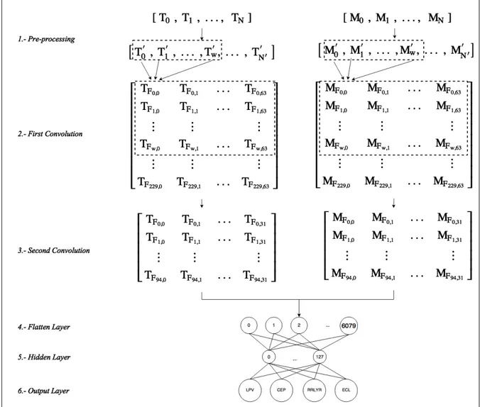
(25) 4. METHOD DESCRIPTION. Figure 4.1. The Convolutional Network Architecture for multi-survey.. We propose an architecture that can classify variable stars using different surveys. We now explain each layer of our architecture, depicted in Figure 4.1. Our architecture transforms each light curve to a matrix representation using the difference between points. We use two convolutional layers for extracting the local patterns and turn them into a flat layer. Two fully connected layers are used, and an output layer is plugged. 15.

(26) at the end to perform the classification. In the following sections, we describe and give insights on each of the layers.. 4.1. Pre-processing In this phase, light curves are transformed into a matrix. Having a balanced dataset is critical for our purpose of multi-survey classification. Therefore, we use NM ax as the maximum number of stars we can extract per class and survey. Section 6.3 explains in detail the selection of the light curves for the database. We transform each of these light curves in a matrix representation of size 2 × N where 2 corresponds to the number of channels (time and magnitude) and N to the number of points used per light curve. Figure 4.2 shows an example of a light curve in a matrix representation. To compare light curves between catalogs a reshape to the matrix must be made. Light curves differ in magnitude and time and for comparing them the difference between observations was used. A matrix of size M × 2 × N was created where M , 2 and N corresponds to the number of light curves, channels, and numbers of observations used. Figure 4.2 shows an example of the transformation of a light curve. Section 6.1 explains in detail this part of the process.. 16.

(27) Figure 4.2. Each light curve is transformed using a matrix with two channels, time and magnitude. For every channel, the maximum number of points is N . Each light curve is transformed using the difference between points and a new matrix is created with two channels.. 4.2. First Convolution We apply a convolutional layer to each of the channels in separate branches with shared weights. We use a shared convolutional layer to preserve the objective of integrating datasets with different cadences. Shared layers mean that each of the filters is the same on every tower. The number of filters is given by S1 . We chose 64 filters, to match the number of 17.

(28) features presented in Nun et al. 2015. The convolution combines our points linearly, creating new ones as follows: sw ∗i+t Xw −1. TFi,j = f (. wk,j ∗ tk + bj ). (4.1). wk,j ∗ mk + bj ). (4.2). k=sw ∗i sw ∗i+t Xw −1. MFi,j = f (. k=sw ∗i. where TFi,j , MFi,j are the time and magnitude after applying the j filter and tk and mk are the time and magnitudes of the light curves. tw is the size of the sliding window and sw the stride value used. Our convolution does not use a max-pooling layer as done in Jiang & Liang 2016. We avoid max-pooling because of the low cadence of Vista Survey and the detriment of losing information. The step function sw was set to 2 or 12 days (considering OGLE cadence of 6 days as average) and the sliding window tw was set to 42 points or 250 days as done in Mackenzie et al. 2016, Valenzuela & Pichara 2017a.. 4.3. Second Convolution After applying one convolution, we employ another one to mix and create more complex features. Jiang & Liang 2016 showed that using two convolutions achieves better results. As in the preceding section, our second convolution is done by linearly combining the time and magnitude of the previous layer: TFi,j = f (. X sw ∗i+t Xw −1. k∈S1. MFi,j = f (. X sw ∗i+t Xw −1. k∈S1. wp,k,j ∗ TFp,k + bj ). (4.3). wp,k,j ∗ MFp,k + bj ). (4.4). p=sw ∗i. p=sw ∗i. where TFi,j and MFi,j are the time and magnitude after applying the second convolution and TFp,k and MFp,k are the time and magnitudes of the first convolution. 18.

(29) As the first convolution, the number of filters is given by S2 , and it was established to be half of the filters used in the first convolution.. 4.4. Flatten Layer After extracting the local patterns, we transform the last convolution into a flatten layer as in Jiang & Liang 2016, Zheng et al. 2014. Our layer combines its patterns afterwards with a hidden layer in a fully connected way.. 4.5. Hidden Layer We use a hidden layer to combine our extracted patterns, and the number of cells is given by ncells . After several experiments, we realize that 128 cells generate the best results. We perform many experiments using sigmoid, relu and tanh activating functions. We obtain the best results using tanh activation, as most of the deep learning literature suggests [LeCun et al., 1998].. 4.6. Softmax Layer In the output layer, there is one node per each of the possible variability classes. We test two different amount of classes: one for 4 classes of variable stars and the other for 9 subclasses. We use a sof tmax function to shrink the output to the [0, 1] range. We can interpret the numbers from the output nodes as the probability that the light curve belongs to the class represented by that node. Finally, we minimize the average across training using categorical cross entropy. We use categorical cross entropy as our loss function as we obtained best results and the datasets use are unbalanced.. 19.

(30) 5. DATA We apply our method to variable star classification using three different surveys: ”The Optical Gravitational Lensing Experiment” (OGLE) [Udalski, 2004], ”The Vista Variable in the Via Lactea” (VVV) [Minniti et al., 2010] and ”Convection, Rotation and planetary Transit” (CoRot) [Baglin et al., 2002, Bordé et al., 2003]. We select these surveys because of their difference in cadence and filters. In the following sections, we explain each of these surveys in detail.. 5.1. OGLE-III The Optical Gravitational Lensing Experiment III (OGLE-III) corresponds to the third phase of the project [Udalski, 2004]. Its primary purpose was to detect microlensing events and transiting planets in four fields: the galactic bulge, the large and small Magellanic clouds and the constellation of Carina. For our experiment, we use 451.972 labeled light curves. The cadence is approximately six days and in the experiments is considered our survey with medium cadence. The band used by the survey is infrared and visible. We discard the visible band because of the low number of observations per star compared to the infrared band. The class distribution is shown in Table 5.1.. 5.2. The Vista Variable in the Vı́a Láctea The Visible and Infrared Survey Telescope (Vista) started working in February 2010 [Minniti et al., 2010]. Its mission was to map the Milky Way bulge and a disk area of the center of the Galaxy. To obtain labeled light curves from Vista, we cross-match the Vista catalog with OGLEIII. We found 246.474 stars in total. The cadence of the observations are approximately every. 20.

(31) Table 5.1. Class distribution of OGLE-III labeled set. Class name Classical Cepheids RR Lyrae Long Period Variables Eclipsing Binaries. Abbreviation Num. of Stars CEP 8.031 RRLyr 44.262 LPV 343.816 ECL 55.863. Subclass Name First-Overtone 10 Classical Cepheid Fundamental-Mode F Classical Cepheid RR Lyrae ab RR Lyrae c Mira Semi-Regular Variables Small Amplitude Red Giants Contact Eclipsing Binary Semi-Detached Eclipsing Binary. Abbreviation Num. of Stars CEP10 CEPF RRab RRc Mira SRV OSARGs EC nonEC. 2.886 4.490 31.418 10.131 8.561 46.602 288.653 51.729 4.134. eighteen days and is considered our survey with low cadence. The band used by the survey is mainly kps , and the class distribution of the labeled subset is shown in Table 5.2. 5.3. CoRoT The Convection, Rotation and planetary Transits (CoRoT) is a telescope launched in December 2016 [Baglin et al., 2002, Bordé et al., 2003]. Its main purpose is to continuously observe the milky way for periods up to 6 months and search for extrasolar planets using transit photometry. One of the main advantages is the high cadence that can be more than a 100 observations per object per day. Because of its early stage, just a few instances have been labeled. For our experiments, we use 1311 labeled light curves. The cadence of the observations are approximately every sixty per day and in the experiments is considered our survey with a high cadence. This catalog does not use any specific filter but the observations per object are in red, blue and 21.

(32) Table 5.2. Class distribution of VVV labelled set. Class name Classical Cepheids RR Lyrae Long Period Variables Eclipsing Binaries. Abbreviation Num. of Stars CEP 36 RRLyr 15.228 LPV 228.606 ECL 2.604. Subclass Name First-Overtone 10 Classical Cepheid Fundamental-Mode F Classical Cepheid RR Lyrae ab RR Lyrae c Mira Semi-Regular Variables Small Amplitude Red Giants Contact Eclipsing Binary Semi-Detached Eclipsing Binary. Abbreviation Num. of Stars CEP10 CEPF RRab RRc Mira SRV OSARGs EC. 5 23 10.567 4.579 8.445 37.366 182.795 1.818. nonEC. 786. Table 5.3. Class distribution of CoRoT labelled set. Class name Classical Cepheids RR Lyrae Long Period Variables Eclipsing Binaries. Abbreviation Num. of Stars CEP 125 RRLyr 509 LPV 109 ECL 568. Subclass Name Abbreviation Num. of Stars RR Lyrae ab RRab 28 RR Lyrae c RRc 481 green bands and for the experiments, we used the white band combining this three. The class distribution is shown in Table 5.3. 22.

(33) 6. EXTRACTION OF DATA In this chapter, we explain in detail how to pre-process the data to produce our inputs. Given that we are integrating several surveys that contain light curves with different bands and number of observations, we have to pre-process the data to get a survey-invariant model.. 6.1. Time & Magnitude Difference The difference between instruments, cadences and bands between surveys create a bias in the variability patterns of light curves [Benavente et al., 2017, Long et al., 2012]. We use as an input the difference between the time and magnitude with the previous measurements. This removes the extinction, distance and survey specific biases. Moreover, it acts as a normalization method. It enables the network to learn patterns directly from the observations without the need to pre-processing any of the data or extinction correction.. 6.2. Light Curve padding The difference in cadence among OGLE-III, Vista, and Corot catalogs create a big variance in the number of observations per light curve. To overcome this problem, we impose a minimum number of observations and use a zero padding to complete the light curves that cannot reach that minimum. This is inspired by the padding procedure done in deep learning for image analysis. To define such limit, we tried many different values and notice that classification results do not change significantly within a range of 500 and 1500 observations. We fixed the limit at 500 points per light curve because that amount preserves the classification accuracy and keeps most of the light curves suitable for our analysis.. 23.

(34) 6.3. A Light curve data augmentation model. Figure 6.1. Example of a new light curve using a burning parameter of 2 and a step parameter of 1.. Hensman & Masko 2015 studied the impact of unbalanced datasets in convolutional neural networks and proved that for better classification performance the dataset should be classbalanced. Since the datasets used in this paper are unbalanced, data augmentation techniques have to be applied [Krizhevsky et al., 2012]. To balance the dataset, we propose a novel data augmentation technique based on light curve replicates. As mention before in Chapter 4, the number of stars per class and survey is given by NM ax . If the number of light curves per class and survey is larger than this parameter, the replication process does not take place. Otherwise, the light curves are replicated until they reach that limit. Each class is replicated using two light curve parameters: burning and step. The burning parameter indicates how many points we have to discard in the light curve. The step parameter tells every how many points we should take samples. The burning parameter goes up every time the light curve has been replicated making the starting point 24.

(35) different for each new data of a specific class and survey. Figure 6.1 shows an example of the replication of a light curve. Is important to note for surveys with high and medium cadences such as Corot and OGLE-III, the loss is not critical as many observations are available. In cases of low cadence catalogs, such as Vista, the loss of observations is significantly reduced depending on the step parameter. To keep a minimum observation loss, the step parameter is set to a random number between 0 and 2. The maximum replication of a light curve is 5.. 25.

(36) 7. PARAMETER INITIALIZATION As in most of deep learning solutions, our architecture needs the set up of several initial parameters. In this chapter, we explain the model design and how to set up its parameters.. 7.1. Parameters As previously noted, surveys have different optics and observation strategies which impact the depth at which they can observe. This impacts the number of variable stars detected and cataloged. In our case, OGLE has been operating longer and observes large portions of the sky while VVV goes deeper but in a smaller area, and Corot has great time resolution but is considerably shallower. The combined catalog is dominated by OGLE stars and the subclasses are highly unbalanced, being the LPV class the majority of them. In order to train with a more balanced dataset, we used a limit of 8.000 stars per class and survey. We tried different values and set it to 8.000 as most of the classes and subclasses of VISTA and OGLE survey possess that amount as shown in Chapter 5. Finally, after several experiments, the batch size was set to 256 for the speed and efficiency in training our algorithm. Table 7.1 shows a summary of the parameters of our architecture.. 7.2. Layers We use two convolutional layers as done in Jiang & Liang 2016. In the imaging literature, several works show that one convolutional layer is not enough to learn a suitable representation, and commonly they use two convolutions [Gieseke et al., 2017, Jiang & Liang, 2016, Zheng et al., 2014]. We try using only one convolution and performance was critically reduced. Three convolutions are also utilized, producing results as good as using two, but the time for training the net and the number of parameters increase significantly.. 26.

(37) A window size tw was used for the convolution process and set to 42 observations or 250 days in average as done in Mackenzie et al. 2016, Valenzuela & Pichara 2017a. Finally, a stride value sw was used and set to 2 or 12 days in average as done in Mackenzie et al. 2016, Valenzuela & Pichara 2017a.. 7.3. Activation functions In convolutional layers we used relu activation function as they are capable of extracting the important information . relu(x). =. max(0, x)). (7.1). For hidden layers, except for convolutional, we used tanh functions because of better results, there widely used and better gradients they provide [LeCun et al., 1998].. 7.4. Dropout Dropout is a regularization technique which randomly drops units in the training phase [Srivastava et al., 2014]. Srivastava et al. 2014 prove the importance of dropout in neural networks to prevent overfitting. We used a dropout of 0.5 as suggested in the mentioned work in the two fully connected parts of our architecture. One between the flattening layer and hidden layer, the other between the hidden layer and the output layer. Dropout increases the generalization of the network, therefore the performance.. 27.

(38) Table 7.1. Parameters used for the proposed architecture Parameter name Global Parameters Stars per survey and class Number of Points Per Light Curve Batch Size Architecture Filters for first convolution Filters for second convolution Window size Stride Value Perceptrons in the hidden layer Dropout Data Augmentation Parameters Burning Step. 28. Abbreviation Value NM ax. 8000. N -. 500 256. S1 S2 tw sw ncells -. 64 32 42 2 128 0.5. burning step. [1,5] [0,2].

(39) 8. RESULTS Our experiments are mainly intended to evaluate the classification accuracy of the datasets described in Chapter 5 as well as the time taken for training the model. We test our model using classes and subclasses and compare it with a Random Forest classifier (RF) [Breiman, 2001], still the most used model for light curve classification [Dubath et al., 2011, Gieseke et al., 2017, Long et al., 2012, Richards et al., 2011]. Our experiments show that unlike RF, our model is scalable as it works with raw magnitudes and time and can be trained iteratively as new light curves arrive. RF needs the extraction of features that takes days or even weeks for training the model. In classification accuracy, our model achieves better results in ECL classes and subclasses and comparable results in LPV and RR Lyrae. RF produces better results in OGLE-III dataset. Fifty-nine features were extracted for each of the surveys using FATS library, computed over 500 observations per light curve. We use the extracted features to train the RF. We perform 10-fold stratified cross-validation on each run. The stratification was done by class and survey to keep the same proportions of classes per survey in the training and testing sets. We perform data augmentation on each of the steps of the cross-validation within the training set. A 20% validation set was used in our model to control the number of epochs during the training process.. 8.1. Computational Run Time As mentioned before, the LSST will start working on 2022 generating approximately 15TB per night. The vast amount of data arriving in the future will demand scalable algorithms. We measure the execution time for each of the classification algorithms, considering the feature extraction (needed just for the RF) and the training iterations. In Table 8.1 we can see that because of the feature extraction needed in RF, that model takes way more time in overall. RF is faster than CNN in the training phase because the CNN needs several epochs,. 29.

(40) Table 8.1. Approximately time of extraction of features and training the algorithms. Method. Extraction Training Total of Features Algorithm Run Time RF 10 days 36 min 10.02 days Clases CNN 30 min 50 min 1.33 hrs SubClases CNN 30 min 91.8 min 2.03 hrs in this case, 500 epochs are needed, where each one takes 6 and 11 seconds to run for classes and subclasses respectively. Our proposed architecture and RF are trained using a computer with 128 GB RAM and a GeForce GTX 1080 Ti GPU. Our algorithm is developed using Keras [Chollet et al., 2015] framework that runs on top of Tensorflow [Abadi et al., 2015] library. We use the scikit-learn [Pedregosa et al., 2011] implementation of RF. We can see that our method is significantly faster as it works with raw magnitudes and time and requires only a couple of minutes of pre-processing. A fundamental characteristic that new algorithms must have is the ability to be incremental, in other words, to be able to deal with new data points without the need of retraining. Moreover, the cost should increase at most in linear time, if not, after few iterations of new arrivals the algorithm would be overwhelmed. Our algorithm scales sub-linearly with new training data points (because it uses mini batches of data in the optimization), while RF scales at least O(nlogn) (considering the orders of time needed in the most expensive feature). As new data arrives, our architecture is capable of training itself with the new data just in seconds instead of re-training the entire algorithm as RF must do.. 8.2. Results with general classes of variability. We test our model using four general classes: (i) Cepheids (CEP), (ii) Long Period Variables (LPV), (iii) RR Lyrae (RRlyr) and (iv) Eclipsing Binaries (ECL). The distribution of classes and subclasses per survey are shown in Tables 5.1, 5.2 and 5.3. Figure 8.2 and 8.3. 30.

(41) Table 8.2. Accuracy per class with the total amount of stars use for each one (in parenthesis). Class ECL-OGLE ECL-VVV ECL-Corot LPV-OGLE LPV-VVV LPV-Corot RRLyr-OGLE RRLyr-VVV RRLyr-Corot CEP-OGLE CEP-VVV CEP-Corot. CNN 0.98 ± 0.01 (8000) 0.92 ± 0.02 (2.604) 0.00 ± 0.00 (1.126) 0.99 ± 0.00 (8.000) 0.94 ± 0.01 (8.000) 0.92 ± 0.11 (109) 0.94 ± 0.01 (8.000) 0.94 ± 0.01 (8.000) 0.00 ± 0.00 (509) 0.90 ± 0.03 (8.000) 0.00 ± 0.00 (36) 0.90 ± 0.08 (125). RF 0.95 ± 0.01 (8.000) 0.30 ± 0.06 (1.184) 0.94 ± 0.03 (1.123) 0.99 ± 0.01 (8.000) 0.98 ± 0.01 (7.596) 0.02 ± 0.04 (101) 0.98 ± 0.01 (8.000) 0.97 ± 0.01 (7.344) 0.21 ± 0.05 (496) 0.94 ± 0.01 (7.374) 0.00 ± 0.00 (23) 0.31 ± 0.11 (121). show the results of using our convolutional architecture and RF respectively. Table 8.2 summarize the accuracy per class of both approaches.. Figure 8.1. Accuracy of the training model using a 10-fold stratified cross validation with classes.. 31.

(42) As it can be seen, RF achieves 96.5% of accuracy in OGLE-III dataset as it has more labeled data than the others surveys. In VVV RF obtains 97% of accuracy in some of the classes that have more labeled data (LPV and RRlyr), but not in stars with few labeled examples (ECL and CEP). In Corot, RF achieves 94% of accuracy only in ECL stars, mainly because of the high cadence of Corot that make it infeasible to extract features correctly, especially those related to periodicity. RF results show that FATS features of some light curves (LPV and RRlyr) can classify accurately between different surveys. That is not a surprise mainly because period features are less sensitive to changes in cadence. Our proposed architecture achieves comparable classification accuracy in OGLE-III but with much less training time. As shown in Figure 8.1 our model produces approximately an accuracy of 97% in the validation set. Each of the colors represents one training of the 10-fold stratified cross-validation. As shown in Table 8.2, OGLE-III dataset achieves 95% of accuracy in average in all of its classes. VVV survey achieves 93.7% of accuracy in most of its classes, except for CEP stars, which are less than 40 light curves. Comparing it to RF performance, it achieves better performance in VVV as it has 92% of accuracy on each of the classes, except for CEP. In Corot, CNN and RF achieve comparable results.. 32.

(43) Figure 8.2. Confusion matrix per class and survey for the convolutional neural network. Empty cells correspond to 0%.. 33.

(44) Figure 8.3. Confusion matrix per class and survey using Random Forest algorithm. Empty cells correspond to 0%.. 8.3. Results with subclasses of variability We test our model using nine types of subclasses: (i) First-Overtone 10 Classical Cepheid (Cep10), (ii) Fundamental-Mode F Classical Cepheid (CepF), (iii) RR Lyrae ab (RRab), (iv) RR Lyrae c (RRc), (v) Mira, (vi) Semi-Regular Variables (SRV), (vii) Small Amplitude. 34.

(45) Red Giants (OSARGs), (viii) Eclipsing Binaries (EC) and (ix) Eclipsing Binaries Semi-Detached (nonEC). The distribution of classes per survey are shown in Tables 5.1, 5.2 and 5.3. Figure 8.5 and 8.6 show the results of using our neural network architecture and Random Forest respectively. Table 8.3 summarize the accuracy per subclass of both approaches.. Figure 8.4. Accuracy of the training model using a 10-fold stratified cross validation with subclasses.. As shown in Figure 8.6, RF achieves accuracies higher than 80% in most of the subclasses in OGLE-III. However, in the VVV survey, 80% is obtained only in RRab and RRc stars. In Corot’s catalog, we have 73% of accuracy in RRc stars, despite the small number of light curves. In Figure 8.4 we can see that our model achieves approximately an accuracy of 85% in the validation set. In OGLE-III dataset, nonEC and Mira stars achieve a 98% of accuracy, and 91.7% in EC, SRV, and Osarg stars. VVV survey achieves 76% of accuracy in RRab and RRc stars, and 94% in Mira stars. However, Osarg and SRV are confused in a 81.3% and 93.2% with Mira type respectively, which indicates a clear overfitting of LPV stars. None of the models can correctly classify VVV Cepheids, mainly because of the low number of light curves (28 light curves in total). With EC and nonEC classes from VVV we achieve better 35.

(46) Table 8.3. Accuracy per subclass with the total amount of stars use for each one (in parenthesis). Subclass EC-OGLE EC-VVV nonEC-OGLE nonEC-VVV Mira-OGLE Mira-VVV SRV-OGLE SRV-VVV Osarg-OGLE Osarg-VVV RRab-OGLE RRab-VVV RRab-Corot RRc-OGLE RRc-VVV RRc-Corot CEP10-OGLE CEP10-VVV CEPF-OGLE CEPF-VVV. CNN 0.93 ± 0.01 (8.000) 0.69 ± 0.04 (1.818) 0.98 ± 0.01 (4.134) 0.51 ± 0.04 (786) 0.98 ± 0.01 (8.000) 0.94 ± 0.01 (8.000) 0.92 ± 0.02 (8.000) 0.00 ± 0.00 (8.000) 0.90 ± 0.01 (8.000) 0.00 ± 0.00 (8.000) 0.72 ± 0.03 (8.000) 0.77 ± 0.02 (8.000) 0.11 ± 0.15 (28) 0.86 ± 0.02 (8.000) 0.75 ± 0.03 (4.579) 0.01 ± 0.01 (481) 0.84 ± 0.03 (2.886) 0.00 ± 0.00 (5) 0.72 ± 0.02 (4.490) 0.00 ± 0.00 (23). RF 0.90 ± 0.01 (8.000) 0.20 ± 0.05 (799) 0.87 ± 0.02 (4.134) 0.03 ± 0.03 (385) 0.98 ± 0.01 (8.000) 0.30 ± 0.02 (4.688) 0.93 ± 0.01 (8.000) 0.67 ± 0.02 (7.575) 0.90 ± 0.01 (8.000) 0.71 ± 0.01 (7.595) 0.97 ± 0.01 (8.000) 0.88 ± 0.02 (7.384) 0.21 ± 0.26 (24) 0.97 ± 0.01 (8.000) 0.84 ± 0.02 (4.071) 0.73 ± 0.05 (472) 0.86 ± 0.03 (2.886) 0.00 ± 0.00 (5) 0.90 ± 0.02 (4.488) 0.00 ± 0.00 (18). results than RF. Finally, the accuracy achieved in Corot is the lowest, mainly because of the few amount of light curves used (28 RRab and 481 RRc stars).. 36.

(47) Figure 8.5. Confusion matrix per class and survey for the convolutional neural network. Empty cells correspond to 0.. 37.

(48) Figure 8.6. Confusion matrix per class and survey using Random Forest algorithm. Empty cells correspond to 0.. 38.

(49) 9. CONCLUSION In this work, we have presented a CNN architecture to classify variable stars, tested on light curves integrated from various surveys. The proposed model can learn from the sequence of differences between magnitude and time, automatically discovering patterns across light curves even with odd cadences and bands. We show that multi-survey classification is possible with just one architecture and we believe it deserves further attention soon. The proposed model is comparable to RF in classification accuracy but much better in scalability. Also, our approach can correctly classify most of the classes and subclasses of variability. Feature description such as FATS are a reasonable way to represent light curves, but the vast amount of time and effort needed to extract them make it infeasible for huge databases. Like most of deep learning approaches, our model is capable of learning its light curve representation, allowing astronomers to use the raw time series as inputs. As future work, oversampling techniques should be studied, given that we observe that our model is sensitive to unbalanced training sets. Also, more complex architectures must be developed to improve classification accuracy. New approaches able to deal with few light curves in some classes are needed. For example, simulation models based on astrophysics would be a significant contribution especially for the most unrepresented subclasses of variability. With simulation models, deep learning architectures could be significantly improved, given that usually their performance is directly related to the number of training cases, even with simulated instances. In the same direction, it would be interesting to produce larger training sets by integrating a higher number of surveys. Our code implementation is done in Python, available for download at https://github.com/C-Aguirre017/ DeepMultiSurveyClassificationOfVariableStars. We also published the catalogs with the cross-matched training sets used in this work.. 39.

(50) REFERENCES. Abadi, M., Agarwal, A., Barham, P., Brevdo, E., Chen, Z., Citro, C., . . . Zheng, X. (2015). TensorFlow: Large-scale machine learning on heterogeneous systems.. Retrieved from. https://www.tensorflow.org/ (Software available from tensorflow.org) Abell, P. A., Allison, J., Anderson, S. F., Andrew, J. R., Angel, J. R. P., Armus, L., . . . others (2009). Lsst science book, version 2.0. arXiv preprint arXiv:0912.0201. Baglin, A., Auvergne, M., Barge, P., Buey, J.-T., Catala, C., Michel, E., . . . others (2002). Corot: asteroseismology and planet finding. In Stellar structure and habitable planet finding (Vol. 485, pp. 17–24). Basheer, I., & Hajmeer, M. (2000). Artificial neural networks: fundamentals, computing, design, and application. Journal of microbiological methods, 43(1), 3–31. Belokurov, V., Evans, N. W., & Du, Y. L. (2003). Light-curve classification in massive variability surveysi. microlensing. Monthly Notices of the Royal Astronomical Society, 341(4), 1373–1384. Benavente, P., Protopapas, P., & Pichara, K. (2017). Automatic survey-invariant classification of variable stars. The Astrophysical Journal, 845(147), 18pp. Bloom, J., & Richards, J. (2011). Data mining and machine-learning in time-domain discovery & classification. Advances in Machine Learning and Data Mining for Astronomy. Bordé, P., Rouan, D., & Léger, A. (2003). Exoplanet detection capability of the corot space mission. Astronomy & Astrophysics, 405(3), 1137–1144. Borne, K. D., Strauss, M., & Tyson, J.. (2007).. Data mining research with the lsst.. BULLETIN-AMERICAN ASTRONOMICAL SOCIETY, 39(4), 137. Breiman, L. (2001). Random forests. Machine learning, 45(1), 5–32. Cabrera-Vives, G., Reyes, I., Förster, F., Estévez, P. A., & Maureira, J.-C. (2017). Deep-hits: Rotation invariant convolutional neural network for transient detection. The Astrophysical Journal, 836(1), 97. Chollet, F., et al. (2015). Keras. https://github.com/fchollet/keras. GitHub. 40.

(51) Cybenko, G. (1989). Approximation by superpositions of a sigmoidal function. Mathematics of Control, Signals, and Systems (MCSS), 2(4), 303–314. De Boer, P.-T., Kroese, D. P., Mannor, S., & Rubinstein, R. Y. (2005). A tutorial on the cross-entropy method. Annals of operations research, 134(1), 19–67. Debosscher, J., Sarro, L., Aerts, C., Cuypers, J., Vandenbussche, B., Garrido, R., & Solano, E. (2007). Automated supervised classification of variable stars-i. methodology. Astronomy & Astrophysics, 475(3), 1159–1183. Dieleman, S., Willett, K. W., & Dambre, J. (2015). Rotation-invariant convolutional neural networks for galaxy morphology prediction. Monthly notices of the royal astronomical society, 450(2), 1441–1459. Dubath, P., Rimoldini, L., Süveges, M., Blomme, J., López, M., Sarro, L., . . . others (2011). Random forest automated supervised classification of hipparcos periodic variable stars. Monthly Notices of the Royal Astronomical Society, 414(3), 2602–2617. Gieseke, F., Bloemen, S., van den Bogaard, C., Heskes, T., Kindler, J., Scalzo, R. A., . . . others (2017). Convolutional neural networks for transient candidate vetting in large-scale surveys. Monthly Notices of the Royal Astronomical Society, stx2161. Graves, A., Mohamed, A.-r., & Hinton, G. (2013). Speech recognition with deep recurrent neural networks. In Acoustics, speech and signal processing (icassp), 2013 ieee international conference on (pp. 6645–6649). Hensman, P., & Masko, D. (2015). The impact of imbalanced training data for convolutional neural networks. Degree Project in Computer Science, KTH Royal Institute of Technology. Hornik, K. (1991). Approximation capabilities of multilayer feedforward networks. Neural networks, 4(2), 251–257. Huijse, P., Estevez, P. A., Protopapas, P., Principe, J. C., & Zegers, P. (2014). Computational intelligence challenges and applications on large-scale astronomical time series databases. IEEE Computational Intelligence Magazine, 9(3), 27–39. Jean, S., Cho, K., Memisevic, R., & Bengio, Y. (2014). On using very large target vocabulary for neural machine translation. arXiv preprint arXiv:1412.2007. Jiang, Z., & Liang, J. (2016). Cryptocurrency portfolio management with deep reinforcement 41.

(52) learning. arXiv preprint arXiv:1612.01277. Kim, D.-W., & Bailer-Jones, C. A. (2016). A package for the automated classification of periodic variable stars. Astronomy & Astrophysics, 587, A18. Kim, D.-W., Protopapas, P., Bailer-Jones, C. A., Byun, Y.-I., Chang, S.-W., Marquette, J.-B., & Shin, M.-S. (2014). The epoch project-i. periodic variable stars in the eros-2 lmc database. Astronomy & Astrophysics, 566, A43. Kingma, D., & Ba, J. (2014). Adam: A method for stochastic optimization. arXiv preprint arXiv:1412.6980. Krizhevsky, A., Sutskever, I., & Hinton, G. E. (2012). Imagenet classification with deep convolutional neural networks. In Advances in neural information processing systems (pp. 1097–1105). LeCun, Y., Bengio, Y., & Hinton, G. (2015). Deep learning. Nature, 521(7553), 436–444. LeCun, Y., Bottou, L., Orr, G. B., & Müller, K.-R. (1998). Efficient backprop. In Neural networks: Tricks of the trade (pp. 9–50). Springer. Long, J. P., El Karoui, N., Rice, J. A., Richards, J. W., & Bloom, J. S. (2012). Optimizing automated classification of variable stars in new synoptic surveys. Publications of the Astronomical Society of the Pacific, 124(913), 280. Machin, J., Pichara, K., Protopapas, P., Neyém, A., & Pieringer, C. (2018). A Global Data Warehouse for Astronomy. Monthly Notices of the Royal Astronomical Society. Mackenzie, C., Pichara, K., & Protopapas, P. (2016). Clustering-based feature learning on variable stars. The Astrophysical Journal, 820(2), 138. Mahabal, A., Sheth, K., Gieseke, F., Pai, A., Djorgovski, S. G., Drake, A., . . . others (2017). Deep-learnt classification of light curves. arXiv preprint arXiv:1709.06257. Minniti, D., Lucas, P., Emerson, J., Saito, R., Hempel, M., Pietrukowicz, P., . . . others (2010). Vista variables in the via lactea (vvv): The public eso near-ir variability survey of the milky way. New Astronomy, 15(5), 433–443. Naul, B., Pérez, F., Bloom, J. S., & van der Walt, S. (2017). A recurrent neural network for classification of unevenly sampled variable stars. Nature Astronomy, 1. Nun, I., Pichara, K., Protopapas, P., & Kim, D.-W. (2014). Supervised detection of anomalous 42.

(53) light curves in massive astronomical catalogs. The Astrophysical Journal, 793(1), 23. Nun, I., Protopapas, P., Sim, B., Zhu, M., Dave, R., Castro, N., & Pichara, K. (2015). Fats: Feature analysis for time series. arXiv preprint arXiv:1506.00010. Pedregosa, F., Varoquaux, G., Gramfort, A., Michel, V., Thirion, B., Grisel, O., . . . Duchesnay, E. (2011). Scikit-learn: Machine learning in Python. Journal of Machine Learning Research, 12, 2825–2830. Pichara, K., & Protopapas, P. (2013). Automatic classification of variable stars in catalogs with missing data. The Astrophysical Journal, 777(2), 83. Pichara, K., Protopapas, P., Kim, D.-W., Marquette, J.-B., & Tisserand, P. (2012). An improved quasar detection method in eros-2 and macho lmc data sets. Monthly Notices of the Royal Astronomical Society, 427(2), 1284–1297. Pichara, K., Protopapas, P., & León, D. (2016). Meta-classification for variable stars. The Astrophysical Journal, 819(1), 18. Pichara, K., Protopapas, P., & Leon, D. (2016). Meta-classification for variable stars. The Astrophysical Journal, 819(1). Ren, S., He, K., Girshick, R., & Sun, J. (2015). Faster r-cnn: Towards real-time object detection with region proposal networks. In Advances in neural information processing systems (pp. 91–99). Richards, J. W., Starr, D. L., Butler, N. R., Bloom, J. S., Brewer, J. M., Crellin-Quick, A., . . . Rischard, M. (2011). On machine-learned classification of variable stars with sparse and noisy time-series data. The Astrophysical Journal, 733(1), 10. Ruder, S. (2016). An overview of gradient descent optimization algorithms. arXiv preprint arXiv:1609.04747. Sarro, L., Debosscher, J., López, M., & Aerts, C. (2009). Automated supervised classification of variable stars-ii. application to the ogle database. Astronomy & Astrophysics, 494(2), 739– 768. Srivastava, N., Hinton, G. E., Krizhevsky, A., Sutskever, I., & Salakhutdinov, R. (2014). Dropout: a simple way to prevent neural networks from overfitting. Journal of machine learning research, 15(1), 1929–1958. 43.

(54) Sutskever, I., Vinyals, O., & Le, Q. V. (2014). Sequence to sequence learning with neural networks. In Advances in neural information processing systems (pp. 3104–3112). Szegedy, C., Liu, W., Jia, Y., Sermanet, P., Reed, S., Anguelov, D., . . . Rabinovich, A. (2015). Going deeper with convolutions. In Proceedings of the ieee conference on computer vision and pattern recognition (pp. 1–9). Udalski, A. (2004). The optical gravitational lensing experiment. real time data analysis systems in the ogle-iii survey. arXiv preprint astro-ph/0401123. Valenzuela, L., & Pichara, K. (2017a). Unsupervised classification of variable stars. Monthly Notices of the Royal Astronomical Society. Valenzuela, L., & Pichara, K. (2017b). Unsupervised classification of variable stars. Monthly Notices of the Royal Astronomical Society. Werbos, P. J. (1990). Backpropagation through time: what it does and how to do it. Proceedings of the IEEE, 78(10), 1550–1560. Xiong, W., Droppo, J., Huang, X., Seide, F., Seltzer, M., Stolcke, A., . . . Zweig, G. (2016).. Achieving human parity in conversational speech recognition.. arXiv preprint. arXiv:1610.05256. Xiong, W., Droppo, J., Huang, X., Seide, F., Seltzer, M., Stolcke, A., . . . Zweig, G. (2017). The microsoft 2016 conversational speech recognition system. In Acoustics, speech and signal processing (icassp), 2017 ieee international conference on (pp. 5255–5259). Zeiler, M. D., & Fergus, R. (2014). Visualizing and understanding convolutional networks. In European conference on computer vision (pp. 818–833). Zheng, Y., Liu, Q., Chen, E., Ge, Y., & Zhao, J. L. (2014). Time series classification using multi-channels deep convolutional neural networks. In International conference on web-age information management (pp. 298–310).. 44.

(55)