Unveiling Exoplanet Atmospheres with the ACCESS Survey

Texto completo

(1)Facultad de Física Instituto de Astrofísica. Unveiling Exoplanet Atmospheres with the ACCESS Survey by NÉSTOR ESPINOZA PEREZ Presented to the Instituto de Astrofísica at the Pontificia Universidad Católica de Chile in partial fulfillment of the requirements for the degree of Doctor of Philosophy. Thesis Advisor: Dr. Andrés Jordán. September, 2017 Santiago, Chile ©2017, Néstor Espinoza Perez.

(2) Se autoriza la reproducción total o parcial, con fines académicos, por cualquier medio o procedimiento, incluyendo la cita bibliográfica del documento.

(3) Unveiling exoplanet atmospheres with the ACCESS Survey by. Néstor A. Espinoza Perez B.Sc., Pontificia Universidad Católica de Chile (2012) Licenciate in Astronomy, Pontificia Universidad Católica de Chile (2012) Submitted to the Instituto de Astronomía y Astrofísica in partial fulfillment of the requirements for the degree of Doctor of Philosophy at the PONTIFICIA UNIVERSIDAD CATOLICA DE CHILE September 2017 c Pontificia Universidad Catolica de Chile 2017. All rights reserved. ○. Author . . . . . . . . . . . . . . . . . . . . . . . . . . . . . . . . . . . . . . . . . . . . . . . . . . . . . . . . . . . . . . Instituto de Astronomía y Astrofísica September 22, 2017. Certified by . . . . . . . . . . . . . . . . . . . . . . . . . . . . . . . . . . . . . . . . . . . . . . . . . . . . . . . . . Andrés Jordán Associate Professor Thesis Supervisor. Accepted by . . . . . . . . . . . . . . . . . . . . . . . . . . . . . . . . . . . . . . . . . . . . . . . . . . . . . . . . . Alejandro Clocchiatti Director de postgrado, Instituto de Astrofísica.

(4) 2.

(5) Unveiling exoplanet atmospheres with the ACCESS Survey by Néstor A. Espinoza Perez Submitted to the Instituto de Astronomía y Astrofísica on September 22, 2017, in partial fulfillment of the requirements for the degree of Doctor of Philosophy. Abstract In this thesis, we present the first results of a survey aimed at the detection of exoplanet atmospheres from the ground using the technique of transmission spectroscopy: the ArizonaCfA-Católica Exoplanet Spectroscopy Survey (ACCESS), a multi-institutional effort aimed at the detection of optical features in giant exoplanet atmospheres. The survey is currently being carried out using the Inamori-Magellan Areal Camera and Spectrograph (IMACS) mounted on the Magellan Baade 6.5m telescope at Las Campanas Observatory, Chile, an instrument not designed (or comissioned) for the precise observations requiered to detect these signatures on these distant worlds, this thesis presents the first detailed comissioning and validation of this instrument for such observations, for which a special data reduction pipeline had to be created and which is today used routinely by the group. In this work we also present a detailed analysis of important stellar astrophysical effects that impact on the observed lightcurve of a transiting exoplanet, which is what is used in practice to extract the signatures of atomic and/or molecular features in the atmospheres of exoplanets using the technique of transmission spectroscopy. In particular, we present two detailed works published in the context of this thesis on the effect of limb-darkening, a fundamental effect observed during the transit of an exoplanet in front of a star, in which we detail how this effect impacts on the retrieved transit parameters, how well we actually understand this effect and how to optimally analyze a transit lightcurve using the “best" parametrization for it, avoiding in this way any biases that might arise from an incorrect treatment of the effect. Thesis Supervisor: Andrés Jordán Title: Associate Professor. 3.

(6) 4.

(7) Acknowledgments Almost any graduate student knows that getting a PhD is mostly about persistence and perseverance, qualities that are often blurred in the face of failure, a very common endproduct during the PhD. I want to start this acknowledgment section by thanking all the people that were there to lift up my spirit during those times, both hearing about the crazy things I was trying out for my research or simply distracting me with the beautiful simple things in life. To all my friends but, especially, to my closest friends Boris Martínez, Rafael Brahm and Diego Sandoval: thank you. To my family, who were always there to support and love me: thank you. I want to especially thank the two most important woman in my life, my wife and my mother, whose love, support and deep insight have not only helped me during my whole career, but have supported me in many ways in all the decisions that I have made in it, including the new European adventure we are about to start with my wife: I have no words to express the gratitude for all of this to you. Thank you very, very much. Every PhD student also knows that the environment where one develops the PhD is also very important. I thus want to thank the Institute of Astrophysics (IA) at the Pontificia Universidad Católica de Chile (PUC) and the Millenium Institute of Astrophysics (MAS) for providing such a rich environment for the development of this thesis, where science from many different areas come together and from which I have learned not only physics and astrophysics, which have been (and will be) very useful in my research, but where I also have received huge support from the administrative side both from the IA (from Carmen Gloria, Lilena, Giselle, Mauricio, Cynthia, Mariela, Juan) and MAS (Denisse, Manuela, María José, Makarena, Claudia). All of this was fundamental for this thesis and, without all them, it would not have been the same. This thesis is in many ways also of that people behind it so thank you very, very much. I also want to take the opportunity to thank all the staff at Las Campanas Observatories (LCO), in which I spent many nights both observing and learning about the instruments that provided the rich datasets presented in this thesis: to the administrative staff, especially to Roberto Bermudez, to the telescope operators, especially to Mauricio Martínez, Mauricio Navarrete and Jorge Araya, and all the staff, especially to Dave Osip from which I have learned so much, thank you very, very much. 5.

(8) Working on a great team, as any PhD student also knows, makes everything easier and richer. For this, first and foremost, I want to thank my thesis advisor, Andrés Jordán, for his infinite support not only on this thesis, but on my career in general. Andrés has and will be an integral part of how I approach science because from day one he treated me not as a PhD student, but as a colleague, always asking my opinion on everything, genuinely hearing my ideas and giving his advice more as an opinion than as an order. I think this is the optimal way of training a scientist, because our work is based on peer review, which is exactly how Andrés approached his position as my PhD advisor. I also want to thank all the people in the local IA group that took the time to teach not only me, but also other students about important details such as observing and reducing data. Hats off go especially to Markus Rabus, Vincent Suc and my good friend Rafael Brahm, whose infinite knowledge about the know-how of astronomy forms a fundamental part of the researcher I have become. I cannot end this paragraph without acknowledging all the support of the ACCESS team, especially that of Daniel Apai, Mercedes Lopez-Morales and David Osip, whose guidance and trust on the research I was performing became a motivation to keep performing the work I did in this thesis and that of Benjamin Rackham, which is not only one of the most insightful researchers I know, but also has become a very good friend. To all of you: thank you very, very much. Finally, I want to thank the funding agencies that allowed me to perform the work I did. First to the COmisión Nacional de Investigación Científica Y Tecnológica (CONICYT), which provided me with the PhD fellowship through the CONICYT-PCHA/Doctorado Nacional fellowship that formed the basis for the funding of my PhD. To the BASAL CATA PFB-06, which helped me during the later stages of the writing of the PhD thesis, and to the MAS institute, which provided additional and fundamental financial support for the development of this thesis through the Ministry for the Economy, Development, and Tourism Programa Iniciativa Científica Milenio through grant IC 120009. Being paid for doing what you love is, definitely, the best payment one can receive.. 6.

(9) Contents 1. Introduction 1.1. 1.2. 1.3 2. 31. Exoplanet atmospheres . . . . . . . . . . . . . . . . . . . . . . . . . . . . 37 1.1.1. The Solar System perspective . . . . . . . . . . . . . . . . . . . . 37. 1.1.2. Observing exoplanet atmospheres . . . . . . . . . . . . . . . . . . 38. 1.1.3. C/O ratios and exoplanet atmospheres . . . . . . . . . . . . . . . . 42. 1.1.4. Clouds, hazes and optical absorbers . . . . . . . . . . . . . . . . . 45. Transmission spectroscopy . . . . . . . . . . . . . . . . . . . . . . . . . . 47 1.2.1. Observability . . . . . . . . . . . . . . . . . . . . . . . . . . . . . 47. 1.2.2. Theory . . . . . . . . . . . . . . . . . . . . . . . . . . . . . . . . 50. The ACCESS Survey . . . . . . . . . . . . . . . . . . . . . . . . . . . . . 52. Transmission spectroscopy: stellar astrophysical challenges. 55. 2.1. The transit lightcurve . . . . . . . . . . . . . . . . . . . . . . . . . . . . . 56. 2.2. The impact of stellar heterogeneities . . . . . . . . . . . . . . . . . . . . . 60. 2.3. 2.4. 2.2.1. Occulted stellar heterogeneities . . . . . . . . . . . . . . . . . . . 60. 2.2.2. Unnoculted stellar heterogeneities . . . . . . . . . . . . . . . . . . 64. The impact of limb-darkening . . . . . . . . . . . . . . . . . . . . . . . . 68 2.3.1. Fitting limb-darkening models . . . . . . . . . . . . . . . . . . . . 70. 2.3.2. Measuring the limb-darkening effect from transit lightcurves . . . . 82. 2.3.3. The effect of using fixed LDCs in transit fitting . . . . . . . . . . . 95. 2.3.4. Lessons learned and best-practices . . . . . . . . . . . . . . . . . . 102. Optimal limb-darkening laws for transit applications . . . . . . . . . . . . 105 7.

(10) 2.4.1. Efficient sampling of coefficients from the logarithmic and exponential laws revisited . . . . . . . . . . . . . . . . . . . . . . . . . 107. 2.4.2. Optimal selection of limb-darkening laws . . . . . . . . . . . . . . 115. Appendices. 129. 2.A Least-squares fits to limb-darkening laws . . . . . . . . . . . . . . . . . . 129 2.B Limiting cases for known target limb-darkening laws . . . . . . . . . . . . 131 2.B.1. Limiting coefficient 𝑎 for the linear law when sampling from the non-linear law . . . . . . . . . . . . . . . . . . . . . . . . . . . . 131. 2.B.2. Limiting coefficients 𝑢1 and 𝑢2 for the quadratic law when sampling from the non-linear law . . . . . . . . . . . . . . . . . . . . . . . . 133. 2.C Fitting and sampling from skew-normal distributions given parameter estimates with asymmetrical errorbars . . . . . . . . . . . . . . . . . . . . . . 135. 3. 2.C.1. Fitting a skew-normal distribution to observed estimates . . . . . . 136. 2.C.2. Sampling from a skew-normal with known parameters . . . . . . . 136. Transmission spectroscopy with Magellan/IMACS. 139. 3.1. IMACS and high-precision spectrophotometry . . . . . . . . . . . . . . . . 139. 3.2. tepspec: a pipeline for transmission spectroscopy . . . . . . . . . . . . . 140. 3.3. 3.2.1. Observational design . . . . . . . . . . . . . . . . . . . . . . . . . 140. 3.2.2. Object identification . . . . . . . . . . . . . . . . . . . . . . . . . 146. 3.2.3. Bad Pixel Mask . . . . . . . . . . . . . . . . . . . . . . . . . . . . 149. 3.2.4. Tracing . . . . . . . . . . . . . . . . . . . . . . . . . . . . . . . . 151. 3.2.5. Sky/Background Removal . . . . . . . . . . . . . . . . . . . . . . 156. 3.2.6. Spectral extraction . . . . . . . . . . . . . . . . . . . . . . . . . . 161. 3.2.7. Wavelength Calibration . . . . . . . . . . . . . . . . . . . . . . . . 162. 3.2.8. Lightcurve generation . . . . . . . . . . . . . . . . . . . . . . . . 168. Lightcurve post-processing . . . . . . . . . . . . . . . . . . . . . . . . . . 172 3.3.1. The ensemble photometry method . . . . . . . . . . . . . . . . . . 173. 3.3.2. The PCA method . . . . . . . . . . . . . . . . . . . . . . . . . . . 177. 3.3.3. The “common-mode correction" method . . . . . . . . . . . . . . 181 8.

(11) 3.3.4 3.4. 4. Validation of IMACS for transmission spectroscopy . . . . . . . . . . . . . 192 3.4.1. “White-light" analysis of WASP-18b . . . . . . . . . . . . . . . . 194. 3.4.2. The transmission spectrum of WASP-18b . . . . . . . . . . . . . . 198. An optical transmission spectrum of WASP-19b 4.1. 4.2. 4.3. 5. Noise modelling . . . . . . . . . . . . . . . . . . . . . . . . . . . 187. 203. Data . . . . . . . . . . . . . . . . . . . . . . . . . . . . . . . . . . . . . . 206 4.1.1. Magellan/IMACS observations . . . . . . . . . . . . . . . . . . . . 206. 4.1.2. Additional photometry . . . . . . . . . . . . . . . . . . . . . . . . 208. 4.1.3. Photometric monitoring . . . . . . . . . . . . . . . . . . . . . . . 212. Transit lightcurve analysis . . . . . . . . . . . . . . . . . . . . . . . . . . 216 4.2.1. “White-light" lightcurve analysis . . . . . . . . . . . . . . . . . . . 216. 4.2.2. Wavelength dependant lightcurve analysis . . . . . . . . . . . . . . 222. 4.2.3. Spot/faculae crossing analysis . . . . . . . . . . . . . . . . . . . . 227. The optical transmission spectrum of WASP-19b . . . . . . . . . . . . . . 234 4.3.1. Stellar activity corrections . . . . . . . . . . . . . . . . . . . . . . 234. 4.3.2. Comparison with models and previous works . . . . . . . . . . . . 237. Summary, conclusions and future work. 243. 5.1. Summary of research findings . . . . . . . . . . . . . . . . . . . . . . . . 243. 5.2. Conclusions and implications of our findings . . . . . . . . . . . . . . . . 246. 5.3. Future work . . . . . . . . . . . . . . . . . . . . . . . . . . . . . . . . . . 250. 9.

(12) 10.

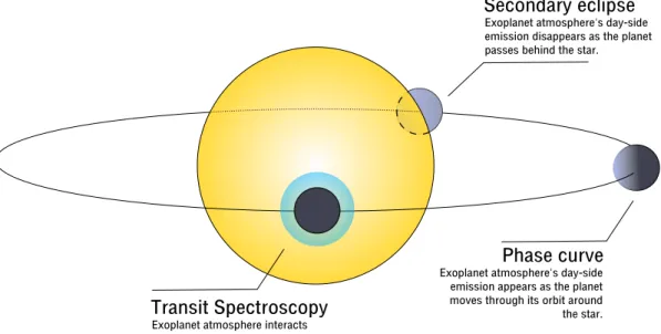
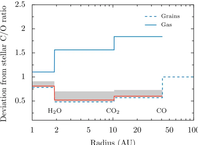
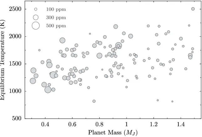
(13) List of Figures. 1-1 Illustration of the methods under which transiting exoplanet atmospheres are currently characterized. For transit (a.k.a. “transmission") spectroscopy, the atmosphere (blue transparent ring around the planet, in grey) has been exaggerated for illustrative purposes. . . . . . . . . . . . . . . . . . . . . . 39. 1-2 Figure from Espinoza et al. (2017) showing the deviation from stellar C/O ratio of solids and grains due to different ice-lines using condensation calculations described in Öberg et al. (2011). The red line with grey bands show the resulting deviation applied to the sample of exoplanets studied in Thorngren et al. (2016) for which estimates for the metal enrichment (and thus, solid and gas enrichment) exists. Ice-lines of H2 O, CO2 and CO are also indicated in the figure. . . . . . . . . . . . . . . . . . . . . . . . . . . 43. 1-3 Figure from Espinoza et al. (2016a) showing a “characterization diagram", that indicates the transmission signals expected from planets in different mass and temperature regimes, updated in order to account for the results of Iyer et al. (2016) who show the observable atmospheres have sizes of 1 ´ 3 scale-heights due to clouds. Sizes of the points indicate 𝛿atm with 𝑎 “ 1, i.e., how “characterizable" an exoplanet is in terms of how big the signals (measured as changes in the transit depth) from their atmospheres would be in transmission. Only planets with 𝑉 ă 14 are shown. . . . . . . . . . . . . 49 11.

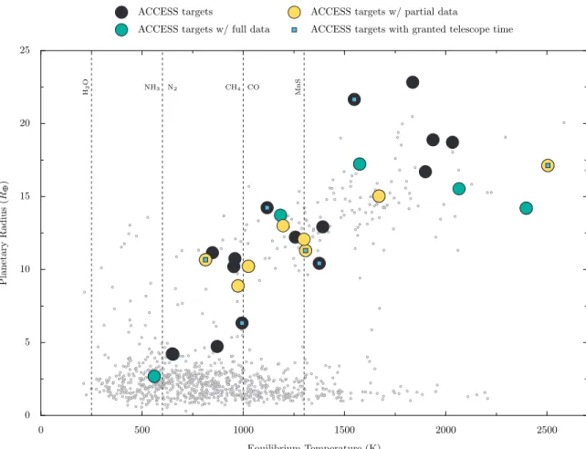
(14) 1-4 Sample planets on the ACCESS survey (big points). Black points indicate planets for which no data has been collected, yellow points indicate planets for which some data has been collected and green points represent systems for which enough data for publication is available. Two of those green points have already been published (Jordán et al., 2013; Rackham et al., 2017). The two other green points are presented in this work. The remining green point is being analyzed by another member of the group. Blue squares represent systems for which telescope time has been granted and small points represent currently known transiting exoplanets. Dashed lines indicate condensation temperatures of different elements on conditions typical in exoplanet atmospheres. . . . . . . . . . . . . . . . . . . . . . . . . . . . . 53. 2-1 Example transit lightcurves obtained for the purposes of this work (colored points) at different wavelenghts (indicated to the right of the lightcurves, in angstroms). The model transit lightcurves (black lines) consider all the parameters of the transit (𝑅𝑝 {𝑅˚ , 𝑎{𝑅˚ , 𝑖, 𝑒, 𝜔) including limb-darkening, which in this case it has been directly obtained from the data (i.e., no stellar models were used in order to predict its effect). Note how the bluest wavelengths show the characteristic “u" shape of the limb-darkening, because the effect is more pronounced at those wavelengths. . . . . . . . . 59. 2-2 Example transit lightcurves where a spot-crossing event is visible, obtained for the purposes of this work (colored points) at different wavelenghts (indicated to the right of the lightcurves, in angstroms). This is the same exoplanet whose transits were shown on Figure 2-1, but in another date. Solid dashed lines show how the transit should look like according to our modelling and solid lines show the full transit model plus the spot model. . 61 12.

(15) 2-3 ATLAS stellar intensity profile obtained for the Kepler bandpass for a G5V type star with solar metallicity (white points), with the colored lines showing fits to the most popular limb-darkening laws. In the upper panel, solid lines correspond to fits obtained following the method of S10, while the dashed lines correspond to fits obtained by following the method of CB11 (note these overlap in the leftmost panels). The lower panel shows the (percentual) difference between these fits. The vertical dashed black line marks 𝜇 “ 0.05 (see text). . . . . . . . . . . . . . . . . . . . . . . . . . . . . . . . . . . . 72 2-4 Limb-darkening coefficients for the quadratic law obtained through the methods described in this work (blue and black), along with previous results by Sing (2010, red) and Claret & Bloemen (2011, green). Below each graph the absolute difference between our results and each previous study is shown, while the difference between those studies is depicted by gray points and between the S10 and CB11 methods (but with our procedures) in black points. Note the large differences in the range 𝑇eff « 7500 ´ 8500 (region denoted by the gray bands) with the Sing (2010) results; this is due to Sing (2010) using old versions of the ATLAS stellar model atmospheres.. 74. 2-5 Differences between LDCs for the quadratic law obtained following the different methods discussed in this work (S10 in red, CB11 in green) and the “real” underlying quadratic LDCs. . . . . . . . . . . . . . . . . . . . . 77 2-6 Close-up to the original (orange squares) and shifted (red squares) limbdarkening profiles for the PHOENIX model atmosphere of a G5V type star with solar metallicity (top) and the derivative of the intensity profile as a a function of 𝑟 “ 1 ´ 𝜇2 (bottom). The black circles show the ATLAS profile for comparison. The dashed line marks the value of 𝑟max found in. this case. . . . . . . . . . . . . . . . . . . . . . . . . . . . . . . . . . . . . 80 2-7 PHOENIX stellar intensity profile obtained for the Kepler bandpass for a G5V type star with solar metallicity (white points). The panels show the same information as Figure 2-3, but for the “shifted” PHOENIX models. . . 81 13.

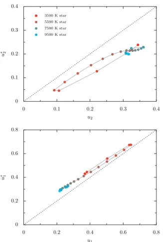
(16) 2-8 Limb-darkening coefficients for the quadratic law obtained through the methods described in this work (blue and black), along with previous results by Claret, Hauschildt & Wittle (2012,2013) in orange (here we plot the coefficients obtained with the “quasi-spherical models”, which only fit values of 𝜇 ě 0.1 using the original PHOENIX intensity profiles); below each graph the absolute difference between our results and this previous study is shown. . . . . . . . . . . . . . . . . . . . . . . . . . . . . . . . . 83. 2-9 Simulation verifying the results of Howarth (2011), where the quadratic LDCs obtained by fitting the intensity profiles from model stellar atmospheres (𝑢1 , 𝑢2 ) for stars with log 𝑔 “ 4.5, r𝑀 {𝐻s “ 0.0 and 𝑣turb “ 2 km/s using the ATLAS models for different temperatures are plotted against these same coefficients (𝑢˚1 , 𝑢˚2 ) obtained from synthetic transit light-curves generated using these same intensity profiles. The gray line follows the temperatures of the simulated systems in increasing order for better visualization. The dashed lines depict the 𝑢𝑖 “ 𝑢˚𝑖 lines, which the points should follow if the coefficients from model intensity profiles and transit lightcurves were directly comparable. . . . . . . . . . . . . . . . . . . . . . . . . . . . 86. 2-10 High (bottom panels) and low (upper panels) precision quadratic LDCs derived from transit photometry for several exoplanets (white datapoints) and MC-SPAM model LDCs p𝑢˚1 , 𝑢˚2 q using ATLAS (blue, to the left of each datapoint) and PHOENIX (red, to the right of each datapoint) models. The blue and red arrows next to the MC-SPAM results represent the mapping 𝑢𝑖 Ñ 𝑢˚𝑖 , i.e., from the original model LDCs obtained from fits to the intensity profiles (in practice obtained using the non-linear coefficients through equation 2.11) and our MC-SPAM estimates. The temperature of the host star of each system is indicated above each of the planet names, inside the figures. Note the change in scale between the upper and lower panels. . . . . . . . . . . . . . . . . . . . . . . . . . . . . . . . . . . . . . 92 14.

(17) 2-11 Differences between the observed LDCs, p𝑢𝑓1 , 𝑢𝑓2 q, shown in Figure 2-10 as white datapoints and the MC-SPAM estimates, p𝑢˚1 , 𝑢˚2 q, using the ATLAS (blue) and PHOENIX (red) models, which are the blue and red points next to the white datapoints in Figure 2-10. Arrows represent the effect of the MC-SPAM algorithm in the observed difference between p𝑢𝑓1 , 𝑢𝑓2 q and the original model LDCs obtained from fits to the intensity profiles. The blue (red) bands indicate the 68% bands around the mean of the differences using the ATLAS (PHOENIX) results (with the median of this indicated by the blue (red) solid line). These medians and the associated 68% values are also indicated next to each band (note that in the upper panels both bands overlap). The dashed black line marks zero, for reference. . . . . . . . . . . 93 2-12 Biases in the recovered planet-to-star radius ratio 𝑝 “ 𝑅𝑝 {𝑅˚ and the semimajor axis-to-stellar radius ratio 𝑎𝑅 “ 𝑎{𝑅˚ as a function of temperature obtained from the simulations described in the text. The upper panels show results when fixing the LDCs, while the lower panels show the results when allowing them to float in the transit light curve fit. The size of the points denote the input value of 𝑝 (𝑝 “ 0.01, small, 𝑝 “ 0.21 big points), while the color of the points represent the input value of 𝑎𝑅 (𝑎𝑅 “ 3.27, blue points, 𝑎𝑅 “ 200 red points). . . . . . . . . . . . . . . . . . . . . . . . . . . . . . 97 2-13 Same as Figure 2-12, but with an impact parameter of 0.3 and an additional panel showing the bias induced on inclination 𝑖. Note that the scale is different than that of Figure 2-12. . . . . . . . . . . . . . . . . . . . . . . . 99 2-14 Same as Figure 2-13, but with an impact parameter of 0.8. Note that the scale is different than that of Figure 2-12, but the same as that of Figure 2-13.100 2-15 Same as Figure 2-12, but with an impact parameter of 0.3 and using LDCs obtained from a different intensity profile (obtained from the work of CB11) to the underlying one (generated using non-linear LDCs from this work). Note that the scale is different from that of previous figures. . . . . . . . . . 101 2-16 Same as Figure 2-15, but with an impact parameter of 0.8. Note that the scale between that figure and this one is also different. . . . . . . . . . . . . 101 15.

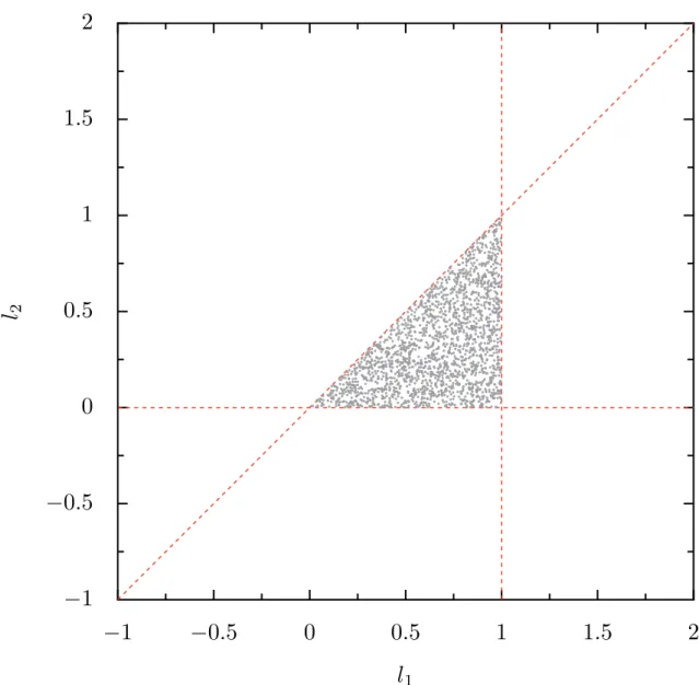
(18) 2-17 Samples of the logarithmic limb-darkening coefficients that satisfy the derived constrains in this section out of 106 uniformly sampled points between ´1 ă 𝑙1 ă 2 and ´1 ă 𝑙2 ă 2. Only „ 5% of those samples satisfy such relations, shown here with red dashed lines. . . . . . . . . . . . 110 2-18 Limb-darkening coefficients for the exponential law obtained using the methods described in the past section with the Kepler bandpass for all the stars in the ATLAS models with 𝑇eff ă 9000 K. As can be seen, 𝑒2 ă 0, which implies that all the fitted intensity profiles are not everywhere positive and, thus, non-physical. . . . . . . . . . . . . . . . . . . . . . . . . . . . . 114 2-19 Results of fitting transit lightcurves with the limb-darkening coefficients as free parameters. Note that the scale shown for the linear law is different than the one used in the figures for the other laws. The size of the points is proportional to the the input values of 𝑝. . . . . . . . . . . . . . . . . . . . 117 2-20 Results of fitting transit lightcurves as described in §3.1 with the limbdarkening coefficients as free parameters, but for low impact parameter transits (𝑏 “ 0.3). Note that the scale shown for the linear law is different than the one used in the figures for the other laws. The size of the points represent the input values of 𝑝, while their color represent the input values of 𝑎𝑅 . . . . . . . . . . . . . . . . . . . . . . . . . . . . . . . . . . . . . . 118 2-21 Results of fitting transit lightcurves as described in §3.1 with the limbdarkening coefficients as free parameters, but for high impact parameter transits (𝑏 “ 0.8). Note that the scale shown for the linear law is different than the one used in the figures for the other laws. The size of the points represent the input values of 𝑝, while their color represent the input values of 𝑎𝑅 . . . . . . . . . . . . . . . . . . . . . . . . . . . . . . . . . . . . . . 119 2-22 Sketch of each of the terms that define the bias and the precision of a given estimator. The probability density of the estimator 𝜃ˆ of the parameter 𝜃 is depicted in red, while the real, underlying value of the parameter 𝜃 is depicted with a black solid line. Ideally, one would want a low bias, high precision estimator. . . . . . . . . . . . . . . . . . . . . . . . . . . . . . . 120 16.

(19) 2-23 Results of our lightcurve fits to noisy lightcurves of a typical Hot-Jupiter in order to study the bias-variance trade-off of different limb-darkening laws on the planet-to-star radius ratio for lightcurves with 100 and 1000 in-transit points. The MSE for different laws is shown as a function of the lightcurve noise level. . . . . . . . . . . . . . . . . . . . . . . . . . . . . . . . . . . 122. 3-1 One of our target stars in this work, WASP-19, with the slit mask already aligned around it. (Left) Image showing a close-up of our target star, WASP19, with the 102 ˆ 202 mask already aligned but before adding the grism which disperses the light. The dashed white line denotes the cut which we plot on the right panel, which shows a cut around the central part of our target star, illustrating the different parts of a typical profile of a Magellan/IMACS observation: the CCD background level (lowest level in counts, around „ 6 ˆ 102 counts in the plot), the sky background on top of this CCD background level (around „ 2 ˆ 103 counts in this plot) and the profile of the star, which is saturated in this image (saturation level of the Mosaic2 CCD camera used in this work is 65, 535 counts). . . . . . . . . . . . . . . 143. 3-2 Throughput of the 300 lines per mm grism with a blaze angle of 17.5 degrees as of December 2016 (D. Osip, private communication). . . . . . . . . . . 143. 3-3 Flowchart of the necessary steps in order to generate the final transmission spectrum from the observations taken with Magellan/IMACS. The reduction steps for which tepspec takes care of are indicated by rounded rectangles. Routines and analysis steps necessary to generate the final transmission spectrum, but outside of tepspec, are indicated by elipses (see text). Important final steps in the process such as the generation of (raw) lightcurves for the target and comparison stars and the generation of the final transmission spectrum are indicated in blue rectangles. . . . . . . . . . . . . . . . . . . 145 17.

(20) 3-4 Object identification in the Mosaic2 chips through the get_mask_coords.py routine. Targets are identified in the plot with white text next to yellow crosses; these crosses are the initial positions given by the user in a text file. This is needed in order for the pipeline to know where to start tracing the spectra and, thus, the user must select a region with high signal to noise. Note also that the same target (e.g., WASP19) can have two positions in the CCD (e.g., WASP19_5 and WASP19_2 in the plot). This is because the spectrum of a target can span two chips in the CCD in the f/2 mode. . . . . 148. 3-5 Bad pixel correction procedure. (Left) Cut in the direction perpendicular to the wavelength direction of a flat frame (blue points), where a bad pixel identified by our algorithm is indicated with a yellow point. (Right) Cut along the direction parallel to the wavelength direction (i.e., in the direction “inside" and “outside" of the left plot) around the position of the bad pixel. In red we plot our interpolation procedure without taking into account the bad pixels in that slice, and the green point denotes the estimated value of the bad pixel, which correctly follows the values around it. Note how this pixel is not the only bad pixel around the same position (those are corrected as well with our procedure). . . . . . . . . . . . . . . . . . . . . . . . . . 150. 3-6 Initial part of our tracing algorithm. The left plot shows a close-up to one of the target stars in one of our datasets, in which the estimated centers of the trace with our algorithm are indicated by blue dots. The center plot shows all the traces estimated by our algorithm in blue points along with a best-fit fourth order polynomial (yellow line), which appears to be a decent fit to the trace. The right panel shows the residuals between that polynomial and the actual estimated centers; note the fit is not perfect but serves, however, for the purposes of this initial fit, which is performed in order to look for outlier points in the trace. . . . . . . . . . . . . . . . . . . . . . . . . . . . 152 18.

(21) 3-7 Variation of the traces as a function of time (frame number in chronological order). (Left) Position of the trace, as measured by the first coefficient in our polynomial fits, as a function of the frame number. Note how the position of the trace slowly decreases in pixel space as a function of time. (Right) Shape of the traces in the image as a function of time. Note how not only the position but the shape also evolves as a function of time. . . . . . . . . 153 3-8 Final simultaneous fit of our tracing algorithm to the trace centers of the target star WASP-19 for the two chips the star spans: chip 2 (left plot) and chip 5 (right plot). Note that the local features not modelled by our polynomial fit are very small, of order „ 0.1 pixels, and we make no attempt to model them, as they are unimportant for the purposes of this work. The overall dispersion of the fit is 0.046 pixels . . . . . . . . . . . . . . . . . . 155 3-9 Profiles observed on science (left) and flat frames (right). As can be observed, both show important levels of scattered light. The causes of this scattered light contamination are still unkown. . . . . . . . . . . . . . . . . 157 3-10 Portion of the stellar, sky and background profile of one of our target stars, WASP-19, as observed from the Mosaic2 CCD camera without any element after the telescope (blue), after putting in the slit mask (orange) and after inserting the dispersive element (green). The black dashed line indicates the background level of each image far away from the target. As can be seen, adding the mask adds a slight widening of the profile. However, adding the dispersive element makes the profile even wider.. . . . . . . . . . . . . . . 158. 3-11 Results of the fit of our model, 𝑆p𝑥q, to the flat field profile. (Left) Data (blue points) against our full model, 𝑆p𝑥q. In the plot we also show the different parts of our model: the step function, 𝐵p𝑥q, and the smooth function (our local background model), 𝑃 p𝑥q. (Right) Residuals of our model. Error bars account for both, photon noise and read-out noise (with the later being negligible). . . . . . . . . . . . . . . . . . . . . . . . . . . . . . . . . . . 160 19.

(22) 3-12 Results of the fit of our local background model, 𝑃𝑠 p𝑥q, to the actual science images. (Left) Data (blue points) against our fitted model for the local background using points outside the slit; the model inside the slit is effectively a prediction of the local background. (Right) Results of the science profile with (blue points) and without (green points) the local background removal (LBR) described in the text. As can be seen, the profile of the sky inside the slit is effectively flat if the LBR model is applied, which demonstrates its power. Points used to remove the background without applying the LBR model (which assumes the background is flat and, hence, only takes the median of 10 points to the left and 10 points to the right of the slit in order to measure the local background) are indicated in yellow. . . . . . . . . . . 161 3-13 Details of the spectral extraction procedure. (Left) The upper panel shows our background and sky-substracted 2-D spectrum, along with the fitted trace (white solid line) and the user-defined aperture (18 pixels in this case, white dashed lines). This is the area that is summed, which gives the spectrum shown in the bottom panel. The deepest line around 350 pixels is H𝛽. The dashed vertical black line shows a cut on the profile shown in the right panel. (Right) Profile illustrating the region used to obtain the target spectrum. The black solid line shows the position of the trace, while the dashed black lines show the aperture over which the profile is summed to produce the final spectrum. Note how the sky level is flat thanks to our local background removal. . . . . . . . . . . . . . . . . . . . . . . . . . . . . . 162 3-14 Results of the initial wavelength calibration procedure, in which the user identifies lines in each of the HeNeAr lamps generated for each target on each chip. The plot shows some of these lines identified by the user. . . . . 164 3-15 Final simultaneous fit to the identified lines in two chips for one of our targets (WASP-19), on the same pixel scale as the trace shown in Figure 3-8. The root-mean-square of our wavelength solution attains the target RMS: 0.046 Angstroms (𝑐∆𝜆{𝜆 „ 2 km/s). . . . . . . . . . . . . . . . . . . . . . 165 20.

(23) 3-16 Wavelength shift of the spectrum of WASP-19 on different chips during the night (science frames ordered in chronological order): on chip 2 (𝛿2 ) and on chip 5 (𝛿5 ). (Top) The panel depicts the wavelength shift of the spectrum of WASP-19 as a function of time. Our smoothing filter, applied to the wavelength shift on chip 5, is also shown. (Middle) Difference between the wavelength shift suffered on WASP-19’s spectrum during the night on chip 2 and on chip 5. As can be seen, the shift is different on chip 2 and on chip 5; the difference being 0.0900 ˘ 0.0045 Angstroms. (Bottom) Difference between the actual observed wavelength shifts for chip 5 and our smoothing filter; as can be seen, our filter correctly follows the shape of this shift. . . . 167 3-17 Final, wavelength-calibrated spectrum of one of our target stars, WASP-19, a G-type star. Some selected prominent lines are depicted in the plot to show that our spectrum has been properly wavelength calibrated, including the O2 telluric A and B bands. Note the gap around 6500 angstroms; this is due to the chip gap between the part of the spectrum captured by chip 2 (𝜆 ă 6500 angstroms) and chip 5 (𝜆 ą 6500 angstroms). . . . . . . . . . . 169 3-18 Anomalous flux level identification by our algorithm, which detects higher or lower levels of flux due to, e.g., cosmic rays, non-identified bad pixels, etc. In this figure, two such flux levels are identified by our algorithm. . . . 170 3-19 Lightcurve generation for one of our targets, WASP-19, from the extracted spectrum. (Top) “White-light" lightcurves for both the comparison stars and WASP-19. Note how the transit of WASP-19b is clearly observed to occur. (Bottom Left) Spectrum of the target star, WASP-19, and the wavelength regions summed in order to generate one point of the lightcurves observed on the right panel. (Bottom Right) Lightcurves generated by summing the light in the wavelength bins indicated in the left panel, normalized and offset for illustrative purposes. The colors of each lightcurve correspond to the wavelength bins depicted under the spectrum in the left panel. . . . . . . . 171 21.

(24) 3-1 Lightcurve post-processing for our “white-light" lightcurve using the “ensemble" method, in which the (6, in this case) comparison stars are weighted in magnitude-space using all the available data. (Left) The left panel shows our target star, WASP-19, as blue points. The best-fit model including the ensemble stars, a magnitude zero-point 𝑍0 and a transit model, is shown in yellow. The comparison stars used to form this ensemble are shown as black lines, and are offset for illustration. (Right) Resulting lightcurve after removing (i.e., dividing) our best-fit ensemble (note this figure does not have the same scale as the left plot). (Bottom) Residuals of our best-fit ensemble + transit model. The rms precision in this case is 272 ppm on 30 second exposures. . . . . . . . . . . . . . . . . . . . . . . . . . . . . . . . . . . . 176 3-2 Same as Figure 3-1, but for the “PCA" method. (Top) The signals obtained through PCA, ordered from the most important on top to the least important at the bottom of the figure. (Bottom) Same results as the ones shown in Figure 3-1, but for the PCA approach. The rms precision in this case is 276 ppm. . . . . . . . . . . . . . . . . . . . . . . . . . . . . . . . . . . . . . . 180 3-3 Light-curve post-processing for our “white-light" lightcurve using the “commonmode" (CM) correction method. (Top) The signals preferred by the model. From left to right, top to bottom: the square of the rotator angle, the square of the shift in wavelength of the spectrum, the full-width at half maximum of the spectrum and the square of the time. Amplitudes are in normalized units. (Bottom) Results of the fit of the signals to the target star (which was divided by one comparison star to remove atmospheric effects). The rms precision in this case is 340 ppm. . . . . . . . . . . . . . . . . . . . . . . . 183 3-4 Resulting wavelength-dependent lightcurves after the raw “atmospheric corrected" lightcurves (i.e., the raw lightcurve of the target star divided by the comparison star, which removes most atmospheric effects) are divided by the common mode model. Note how the lightcurves appear more sharper thanks to the removal of the common mode systematics. . . . . . . . . . . 184 22.

(25) 3-5 Samples from a Gaussian Processes coming from both, an squared exponential kernel (top) and a Matérn 3/2 kernel (bottom), for different characteristic length-scales. The amplitudes for both of the processes is unitary (i.e., 𝜎𝑆𝐸 “ 𝜎𝑀 “ 1). . . . . . . . . . . . . . . . . . . . . . . . . . . . . . . . . 190 3-1 Typical spectrum of WASP-18, as obtained by our pipeline. Observed lines are identified in order to illustrate the correct wavelength calibration of our spectra. Note the chip gap at „ 7000 angstroms. . . . . . . . . . . . . . . . 194 3-2 Transit lightcurve of WASP-18b as observed from Magellan/IMACS on August 17th, 2014. (Top) Data after removing the systematic effects model with our PCA analysis (blue points) along with the best-fit transit model (yellow line). (Bottom) Residuals of our best-fit model in ppm. The rms of the lightcurve is 726 ppm on 3-second exposures. The errobars correspond to the fitted value of 𝜎𝑤 “ 734`25 ´22 ppm. . . . . . . . . . . . . . . . . . . . 195 3-3 Traces of chip 5 of our target star, WASP-18, throughout the night. Compare this plot to the trace changes during the night for WASP-19, shown in Figure 3-7. (Left) Position of the trace in pixel space. Note the high scatter of order „ 0.3 pixels between images (the same scatter is 0.05 for the trace of WASP-19). (Right) Trace shape as a function of time. . . . . . . . . . . . . 196 3-4 Wavelength-dependent transits of WASP-18b with the systematic errors removed from 4900 ´ 9400 Angstroms (colored points, bluer points indicating bluer wavelengths and reddest points indicating larger wavelengths) and best-fit transit models (black solid lines). Note the slight variation of the limb-darkening as a function of wavelength in the lightcurves, with bluer transits having more “u"-shaped transits than redder transits, which show more box-like shapes. Text with the wavelength range of each transit lightcurve is indicated to the right of each lightcurve. . . . . . . . . . . . . 199 3-5 Transmission spectrum of WASP-18b in 200 angstrom bins from 4900 ´ 9400 Angstroms. Note the gap at 7000 angstroms due to the chip gap. Blue band indicates the dispersion around the mean value (𝑅𝑝 {𝑅˚ “ 0.100), which is „ 350 ppm. . . . . . . . . . . . . . . . . . . . . . . . . . . . . . 200 23.

(26) 4-1 Typical spectra of WASP-19, as obtained by our pipeline, for each date of observations (from top to bottom: April 12, 2017, April 4th, 2017, February, 2017, June, 2015, April, 2014 and March 2014) which are offset for clarity. Colors indicate the different setups used in our work (no blocking filter in black, “red" setup in red and “blue" setup in blue; for details, see text). Observed lines are identified in order to illustrate the correct wavelength calibration of our spectra. Note the chip gap at „ 6500 Angstroms. . . . . . 208 4-2 Additional transits of WASP-19b obtained in the context of this project from TRAPPIST (left) and CHAT (right). The blue curve shows the best-fit transit model and the residuals of each fit are presented in the bottom panels (in ppm). Error bars depict photon-noise errors which, in this case, adequately represent the dispersion in the data. . . . . . . . . . . . . . . . . . . . . . . 209 4-3 Photometric monitoring obtained during the 2014 season for WASP-19 from CTIO. The same photometry is shown for a comparison star. Note how the photometry is good only at the „ 1% level, and shows evident night-to-night systematics visible in both, WASP-19 and the comparison star. . . . . . . . 213 4-4 Photometric monitoring obtained during the 2017 season for WASP-19 from ASAS-SN. Upper panel. Photometry of WASP-19, along with vertical bands indicating the epochs at which the Magellan+IMACS observations were carried out: green for the 17/02/11 observations, orange for the 17/04/04 observations and blue for the 17/04/12 observations. The blue curve that goes horizontally through the points is the best-fit Gaussian process used to both retrieve the rotation period of the star and to estimate the relative flux level of WASP-19 at those different epochs (see text). Lower panel. The left lower panel shows a close-up of the photometry and best-fit Gaussian process (see text) to around the epochs of the Magellan+IMACS observations. The right lower panel shows the posterior distribution of the period estimated through our Gaussian-process regression (see text). . . . . . . . . 217 24.

(27) 4-1 White-light transit lightcurves after correcting for our systematics model for all of our Magellan+IMACS observations. The lightcurves on top are the ones obtained with our setup without blocking filters (March and April 2014, June 2015) and the ones on the bottom are taken with blocking filters (February and April 4th, 2017, taken with our “red" setup and the April 12th 2017 dataset taken with our “blue" setup). The small panels below each lightcurve shows the residuals in parts per million (black points with errorbars) and the best-fit noise model (blue curve) for each dataset (straight bands for all the datasets except for the March 2014 dataset, which is consistent with a “granulation" noise model). The blue bands denote the 1-sigma credibility bands of our noise models; errorbars in the panels below each lightcurve correspond to the fitted jitter term (indicated in the figures in ppm), which is consistenly three times above the poisson level for all of our datasets except for the March 2014 dataset, which is only 2 times above the poisson level. The gaps in the April 29th 2014 and 4th of April 2017 datasets are due to star-spot and/or faculae crossings. . . . . . . . . . . . . 219. 4-2 Spot and faculae-crossings as observed on our white-light transit lightcurves. The data used to obtain the transit lightcurve fits is displayed as black points in the top plot, while the points left out of the fit are displayed in blue; the best-fit transit model is also shown in blue. The April 29 2014 data shows the typical brightening of the observed lightcurve typical of spot crossing events and/or additional transiting objects, while the April 2017 lightcurve shows a small dimming, a signature expected for a faculae crossing. The bottom pannel shows the residuals and, in blue, the filtered shape of the spots which is used to model the signatures in the analysis of the lightcurves at each wavelength. . . . . . . . . . . . . . . . . . . . . . . . . . . . . . . 223 25.

(28) 4-3 Transit lightcurves (colored points) after our systematics removal for the 2014 and 2015 season: March, 2014 (left), April, 2014 (center) and June, 2015 (right). Solid lines represent our modelling of these lightcurves, which for the April dataset includes the spot-crossing event. For this last dataset, in dashed lines we also show the transit model without the spot model, in order to illustrate the amplitude of the spot-crossing event at different wavelengths. These datasets were taken without a blocking filter. . . . . . . . . . . . . . 224 4-4 Same as 4-3, but for the 2017 season: February 2017 (left), April 4th, 2017 (center) and April 12th, 2017 (right). The first two wavelength bins on Figure 4-3 are missing here for the two leftmost transits, as those datasets were taken with the “red" setup. Note the faculae-crossing event on the April 4th dataset and the change in scale and wavelength range for the April 12th dataset, whose data was obtained with our “blue" setup, and hence covers our bluest wavelength bins. . . . . . . . . . . . . . . . . . . . . . . 225 4-5 Transmission spectra obtained at the different seasons (black points) compared to the datapoints from all seasons (grey points). The blue datapoint in the April 29, 2014 panel corresponds to the value of 𝑅𝑝 {𝑅˚ retrieved from the TRAPPIST observations on April 25, 2014, while the red datapoint on the April 12, 2017 panel shows the value of 𝑅𝑝 {𝑅˚ retrieved from the transit observed by CHAT on that same day. The season is indicated to the lower right of each panel. Blue bands indicate the mean value of 𝑅𝑝 {𝑅˚ for each season and the population standard-deviation obtained using those wavelength-dependant ratios. Grey dashed vertical lines indicate the wavelengths at which Na and K are expected to be observed. Note the values of 𝑅𝑝 {𝑅˚ presented here have not been corrected for stellar activity. . . . . . . 228 4-6 Modelling of the spot (left) and faculae (right) crossing events with SPOTROD (blue curves) to the data (black points with errorbars). Dashed blue lines represent the transit model which was fixed and found on Section 4.2.1. As can be seen by the residuals (bottom panels), the spot and faculae models are able to capture all the structure observed on the data within the errorbars. 229 26.

(29) 4-7 Illustration of the spot (left) and faculae (right) crossing events as modelled by SPOTROD. The large yellow circle represents the star, while the small dark circle in both representations depicts WASP-19b, with its transit chord represented by dashed lines. The dark spot on the left and white spots on the right represent the size of the spot and faculae, respectively, as measured by SPOTROD. The sizes and positions are shown to scale (relative to the star). The brightness contrasts of the star (including its limb-darkening), the planet, spot and faculae are not to scale. . . . . . . . . . . . . . . . . . . . 230. 4-8 Spot (top) and faculae (bottom) contrasts as a function of wavelength obtained with our SPOTROD fits to the April 29 2014 and April 4 2017 datasets, respectively. Half-violin plots (blue filled curves) denote the posterior probability distribution of the contrasts as obtained from the MCMC fit to the wavelength-dependant lightcurves, with higher densities increasing to the right. The errorbars mark the median (black points) and the 68% credibility bands around this point (black lines). . . . . . . . . . . . . . . . 232. 4-1 Activity correction factor, 𝑎, for the April 4th and 12 2017 datasets (red points with errorbars) and for the February 11 2017 dataset (blue points with errorbars). . . . . . . . . . . . . . . . . . . . . . . . . . . . . . . . . 236. 4-2 Final, combined transmission spectrum of WASP-19b (black points) as measured from 6 transits from Magellan/IMACS (grey points). The combined transmission spectrum has a median precision of 157 ppm in the transit depth.237. 4-3 Magellan/IMACS transmission spectrum (blue points with errorbars) compared with the optical transmission spectrum presented in Huitson et al. (2013) and reanalyzed in Sing et al. (2016) (red points). Clear atmosphere models with TiO (purple) and without TiO (red) are shown as solid lines. Model without TiO and without sodium or hazes is shown in red dashed lines.239 27.

(30) 5-1 Simulated transit of an habitable-zone Earth-sized planet orbiting an Mstar, which produces a 200 ppm signal, and which could be detected with Magellan/IMACS white-light lightcurves. This lightcurve was generated with the residuals of one of our WASP-19b transit lightcurves presented in Chapter 4. . . . . . . . . . . . . . . . . . . . . . . . . . . . . . . . . . . . 248. 28.

(31) List of Tables 2.1. Sample of confirmed Kepler planets for which limb-darkening coefficients have been obtained. . . . . . . . . . . . . . . . . . . . . . . . . . . . . . . 125. 2.2. Parameters of the host stars of each of the planets listed in Table 2.1. . . . . 126. 2.3. Results of the limb-darkening coefficients obtained using the MC-SPAM algorithm. . . . . . . . . . . . . . . . . . . . . . . . . . . . . . . . . . . . 127. 3.1. Comparison stars used for the analysis of WASP-18b’s transit lightcurve . . 194. 3.2. Transit parameters obtained for our white-light transit fit, compared to previous works. For the Spitzer parameters, the errors include both systematic and statistical errors. . . . . . . . . . . . . . . . . . . . . . . . . . . . . . 197. 3.3. Values of 𝑅𝑝 {𝑅˚ from 4900 to 9400 Angstroms, show in Figure 3-5. 𝜆𝑙 stands for the lower limit of the wavelength bin; similarly 𝜆𝑢 stands for the upper limit. . . . . . . . . . . . . . . . . . . . . . . . . . . . . . . . . . . 201. 4.1. Comparison stars used in this study . . . . . . . . . . . . . . . . . . . . . . 206. 4.2. Details of our Magellan/IMACS transit observations of WASP-19b. The “Full" setup indicates a setup in the f/2 mode with the 300+17.5 grism and no blocking filter, thus using the full wavelength range determined by the grism. The “Red" setup indicates the setup in which a blocking filter that has a sharp cutoff at 4550 Angstroms was used together with the mentioned grism and the “Blue" setup indicates a setup, in which we use a blocking filter that has a sharp cutoff at both 3600 and 5700 Angstroms, which was used together with the mentioned grism. 𝑡exp indicates the exposure times. Read-out modes have 30 (Turbo) and 31 (Fast) second read-out times. . . . 207 29.

(32) 4.3. Retrieved transit parameters for the TRAPPIST (14/04/25) and CHAT (17/04/12) observations; 𝑠1 and 𝑠2 stand for the first and second limbdarkening coefficient of the square-root law. Times for the TRAPPIST observations are in HJD. For CHAT in BJD. . . . . . . . . . . . . . . . . . 211. 4.1. Retrieved transit parameters obtained for each of our white-light transits; 𝑠1 and 𝑠2 stand for the first and second limb-darkening coefficient of the square-root law. . . . . . . . . . . . . . . . . . . . . . . . . . . . . . . . . 221. 30.

(33) Chapter 1 Introduction. “. What other conclusion shall we draw from this difference, Galileo, than that the fixed stars generate their light from within, whereas the planets, being opaque, are illuminated from without; that is, to use Bruno’s terms, the former are suns, the latter, moons, or earths?. ”. Johannes Kepler, Dissertatio cum Nuncio Sidereo1 , 1610 Throughout history, scientists, philosophers and theologists have discussed the idea of the existence of worlds other than our own in the universe. Giordano Bruno was perhaps one of the first to seriously consider the idea that there might be stars other than our own Sun in our universe. Even more, he proposed that these stars had planets similar to our own orbiting them, ideas that were perhaps one of the main reasons why he was tried for heresy by the Roman Inquisition (Martinez, 2016), which found him guilty and burned him to death in 1600. Although his ideas were philosopical and theological in nature, today we know he was essentially right: on average, all stars in the Milky Way have at least one planet orbiting them (Cassan et al., 2012). Serious study of the ideas of Bruno had to wait almost 400 years to be tested. It was only in 1992 when the first planet outside our Solar System was detected in a, by all means, 1. As translated in “Kepler’s Conversation with Galileo’s Sidereal Messenger" by E. Rosen in “The Sources of Science", No. 5, 1965..

(34) 32. CHAPTER 1. INTRODUCTION. strange configuration: two planets orbiting a neutron star, discovered through pulsar timing by Wolszczan and Frail (1992). Only three years later, however, the discovery of 51 Pegasi b by Mayor and Queloz (1995), a planet orbiting a Sun-like star only 50 light-years away from our planet, completely changed our view of what “other worlds" actually meant, and started the field that we today know as extrasolar planets (or “exoplanets", for short). The discovery of 51 Pegasi b was profound in many ways. On one hand, it allowed us to confirm the idea that other worlds do exist orbiting around stars similar to our own Sun which, until that time, had only theoretical support. On the other hand, the discovery was at the time in many ways unexpected. 51 Pegasi b is what we know today as a “hot-Jupiter": a short-period („ 4-days) giant planet with a minimum mass about half that of Jupiter. This means that the planet is very close to its star and hence their name. The problem, however, was that the classical core-accretion scenario predicted that these giant planets formed at distances 10 Á AU, where it was easier for them to attain their „ 10𝑀C rocky cores needed in order to start the runaway gas accretion process that finally formed the gas giant planets we observed today in our Solar System (Lissauer, 1993). The big question was how 51 Pegasi b either (1) formed in the position it is observed today or (2) managed to reduce its orbital distance by a factor of „ 10´2 . Although motivated by this and many more similar discoveries today we have a better understanding of the processes of planet formation, which include both theories of how giant planets might migrate from their formation locations (see, e.g., Goldreich and Tremaine, 1980; Lin and Papaloizou, 1986; Rasio and Ford, 1996; Wu and Lithwick, 2011; Fabrycky and Tremaine, 2007; Petrovich, 2015) or how they might even form “in-situ" (Batygin et al., 2016), the debate is still not settled. This discovery is, thus, illustrative on how discoveries in the field of exoplanets have a tremendous importance, as they not only expand what we have learned on the planets in our own Solar System, but also help us to understand how other systems form as well, and what is our place whithin this diverse set of distant worlds. The discovery of 51 Pegasi b also started the race to discover new of these strange worlds. In particular, surveys to detect these distant worlds using the radial-velocity technique (which aims at detecting the doppler shifts on stars caused by planetary companions) – the same method with which 51 Pegasi b was discovered – performed very efficiently in those young.

(35) 33. years of exoplanet detection, discovering tens of planets whithin only a couple of years (see, e.g., Marcy and Butler, 1998, for an overview of the work at the time). The biggest problem with the radial-velocity technique, however, was that it didn’t allow for a further characterization of the exoplanet – at least not with the technology at that time. The composition of the exoplanet, in particular, was not possible to infer from the parameters that the radial-velocity technique allowed us to estimate. In fact the only parameter that had some influence on the composition of the exoplanet retrieved from radial-velocity measurements was 𝑀𝑝 sinp𝑖q, where 𝑀𝑝 is the mass of the planet and 𝑖 is the inclination of the orbit (the angle between the normal to the orbital plane and our line of sight). As a consquence, the mass obtained by this method was only a minimum mass and thus, only loose constrains on the actual composition of exoplanets were allowed to be put in the early years of exoplanet detection. Even before the detection of these first exoplanets, the power of detecting extrasolar planets via the transit method – an alternative (and complementary, as we will see) method to the radial-velocity method, in which one aims to measure the apparent change in the flux of a star as a planet passes in front of it – was readily explored in the literature (Rosenblatt, 1971; Borucki and Summers, 1984; Borucki et al., 1985). It was noted by these early researchers that the ammount of apparent flux the star loses as observed from Earth due to the passage of an exoplanet in front of it which we today call the transit depth, 𝛿, was basically the ratio of the cross sections of both the planet and the star in our direction from Earth, i.e., 𝛿 “ 𝑅𝑝2 {𝑅˚2 , where 𝑅𝑝 is the planetary radius and 𝑅˚ is the stellar radius. Furthermore, if this (lucky) alignment indeed happens, then 𝑖 „ 90 and, thus, using the radial-velocity technique, an estimate for the absolute (or “true") mass of the planet, 𝑀𝑝 , could be obtained. With knowledge of the stellar radii, the transit method would then yield 𝑅𝑝 which, combined with the measurement of the true mass using the radial-velocity method, would allow for an estimation of the density of the exoplanet, 𝜌 „ 3𝑀𝑝 {4𝜋𝑅𝑝3 : a first-order measurement of an exoplanet’s composition. As recognized by Borucki and Summers (1984), however, discovering a planet using this technique was hard: assuming all orbits are equally probable from our perspective at Earth, the probability of observing a planetary transit is P𝑇 „ 𝑅˚ {𝑎, where 𝑎 is the semi-major axis of the orbit. For a planet on an Earth-like orbit around a.

(36) 34. CHAPTER 1. INTRODUCTION. Sun-like star, for example, P𝑇 „ 0.5%. For a short-period hot-Jupiter, however, where a 51 Pegasi b-like planet orbits a Sun-like star, 𝑎 „ 0.05 AU, and thus the probability is boosted to P𝑇 „ 10%. This was noted by researchers shortly after the discovery of these hot-Jupiters, which initiated follow-up campaigns on these radial-velocity detected exoplanets in order to look for transits, whose initial efforts yielded no transits for several planet-hosting stars, including 51 Pegasi b (see, e.g., Baliunas et al., 1997; Henry et al., 1997, 2000a). The first observation of a transit of an exoplanet had to wait 5 years after the discovery of 51 Pegasi b. These were simultaneously reported by Henry et al. (2000b) and Charbonneau et al. (2000), who reported transits of the exoplanet HD209458b, discovered via the radialvelocity method by Mazeh et al. (2000). This allowed, for the first time, to measure the “true" radius („ 1.3𝑅𝐽 ), mass („ 0.6𝑀𝐽 ) and thus density of an exoplanet, which in this case was 𝜌 „ 0.4 gr/cm3 , which is significantly lower than both Jupiter and Saturn. This was somewhat expected, as the radii of these highly irradiated giant exoplanets was predicted to be larger than the radii of our solar system giant planets and, thus, their densities were expected to be lower than the gas giants observed in our Solar System well before this first measurement of an exoplanetary radius (Guillot et al., 1996). The composition of the exoplanet, now confirmed to be consistent (as expected) with an hydrogen/helium (H/He) dominated gas giant planet, however, was still consistent with a wide range of possible compositions. The mass and radius was, thus, still not enough information in order to explore what the exoplanet was actually made of (Guillot et al., 1996; Goukenleuque et al., 2000; Burrows et al., 2000). Whithin months of the discovery of this first transiting extrasolar planet – as we now call them – Seager and Sasselov (2000) pointed out a very interesting fact about them: during a transit, light also passes through an exoplanet atmosphere and, thus, light that interacted with this atmosphere reaches us at Earth allowing us, in principle, to detect the small spectroscopic signatures the exoplanet atmosphere imprints on the stellar light. Transits thus did not only allow first order estimates of the exoplanet composition from derived values such as the density: they also open a window through which we can actually detect their atmospheres, allowing us to detect atomic and/or molecular features in these distant worlds from the comfort of our pale blue blue dot. Two years after this prediction,.

(37) 35. Charbonneau et al. (2002) reported the first detection of an exoplanet atmosphere using this technique – today known as transmission spectroscopy – on the exoplanet HD209458b with the Space Telescope Imaging Spectrograph (STIS) mounted on the Hubble Space Telescope (HST): sodium was found to be present in HD209458b, allowing us to put the first constraint on an atmosphere of a distant world in the history of human kind. Since this first detection of an exoplanet atmosphere, the field grew tremendously in the subsequent fifteen years (see Crossfield, 2015, for a detailed overview). Fueled by the discoveries of hundreds of characterizable transiting extrasolar planets by surveys such as HATNet (Bakos et al., 2004), HATSouth (Bakos et al., 2013) and WASP (Pollacco et al., 2006), there is today a plethora of new worlds whose atmospheres can be characterized and, at last, understood in the context of their formation and evolution. We are living, thus, in the golden age of the field of exoplanets. This exciting reality is what motivates the present work. In this thesis, we present the first results of a survey aimed at the detection of exoplanet atmospheres from the ground using the technique of transmission spectroscopy: the ArizonaCfA-Católica Exoplanet Spectroscopy Survey (ACCESS). The survey, which is a multiinstitutional effort, aims at the detection of optical features in these exoplanet atmospheres, focusing especially on short-period giant exoplanet atmospheres which, as we will see in the next section, are of special importance for a number of reasons. The survey is currently using the Inamori-Magellan Areal Camera and Spectrograph (IMACS) mounted on the Magellan Baade 6.5m telescope at Las Campanas Observatory, Chile (Dressler et al., 2006, 2011), which is an instrument not designed (or comissioned) for the precise observations required to detect these signatures on these distant worlds. As such, this thesis presents the first detailed comissioning and validation of this instrument for such observations, for which a special data reduction pipeline had to be created and which is today used routinely by the group (see Jordán et al., 2013; Rackham et al., 2017). In this thesis, we also present a detailed analysis of important stellar astrophysical effects that impact on the observed lightcurve of a transiting exoplanet which, as we will explain in the following sections, is what is used in practice to extract the signatures of atomic and/or molecular features in the atmospheres of exoplanets using the technique of transmission spectroscopy. In particular,.

(38) 36. CHAPTER 1. INTRODUCTION. we present two detailed works published in the context of this thesis (Espinoza and Jordán, 2015, 2016) on the effect of limb-darkening, a fundamental effect observed during the transit of an exoplanet in front of a star, in which we detail how this effect impacts on the retrieved transit parameters, how well we actually understand this effect and how to optimally analyze a transit lightcurve using the “best" parametrization for it, avoiding in this way any biases that might arise from an incorrect treatment of the effect.. This work is organized as follows. In the following sections of this first chapter we give an overview of exoplanet atmospheres, the challenges it poses from an observational and theoretical perspective, and a brief introduction to the theory of transmission spectroscopy, ending the chapter with a presentation of the ACCESS survey including its objectives and the sample under study. In Chapter 2 we present the stellar astrophysical challenges that appear in the study of the transmission spectra of exoplanets, including our work on limbdarkening, but also including a section on the impact of stellar activity. Chapter 3 presents a detailed explaination of our observations with Magellan/IMACS, and we present the dedicated pipeline created for transiting extrasolar planet spectroscopy (tepspec), which we wrote for Magellan/IMACS, but which is flexible enough to be ported to any multi-object spectrograph for this and other purposes. In this chapter, we also present a validation study in which we test our algorithms on an exoplanet with known (null) atmospheric features. Chapter 4 presents a detailed study of the optical transmission spectrum of WASP-19 as observed from Magellan/IMACS on 6 different epochs, with which we not only obtained a very precise combined transmission spectrum which gives important constraints on the atmosphere of this exoplanet, but also tests the long-term stability of the instrument for this kind of study. We end this work with Chapter 5, in which we present a summary of the studies performed whithin ACCESS, and discuss future work to be performed with this and other projects..

(39) 1.1. EXOPLANET ATMOSPHERES. 1.1 1.1.1. Exoplanet atmospheres The Solar System perspective. The study of the atmospheres of worlds other than our own is best introduced with the large ammount of studies performed on the atmospheres of our Solar System planets. In particular, the study of the atmospheres of our giant planets is of special importance from the perspective of the formation of our Solar System, as they have primordial (or primary) atmospheres, which were accreted during the formation of our Solar System, 4,500 million years ago, in contrast with the rocky planets such as Earth’s, whose – secondary – atmospheres have substantially changed from their accreted primary atmospheres due to the outgassing of material contained within the rocky material that forms their bulk composition (Seager and Deming, 2010). As such, our Solar System giant planets are relics of the formation process that made the Solar System that we see today. One of the most important lessons we have learned from the study of the atmospheres of our Solar System giant planets is that their compositions do not follow the composition of the Sun (Atreya et al., 2016). In particular, the elemental abundances in Jupiter (determined through the Galileo Probe), Saturn (determined using data from the Cassini mission), Uranus and Neptune (both determined using data from HST, with extra data from radio occultations by Voyager for the former) seem to be enriched with respect to the protosolar nebula, with Jupiter having on average „ 4 times the abundance of elements heavier than hydrogen and helium in its atmosphere, Saturn having „ 9 ´ 10 times the abundance of the same elements and Uranus and Neptune having „ 80 times the abundance of carbon in its atmosphere when compared to protosolar nebular abundances. This is evidence that planetesimals, which carry mostly heavy elements, actually polluted the gas accreted from the initial protosolar nebula that formed their atmospheres and, thus, the exact make-up and enrichment of the different elements in their atmospheres is key to the understanding of how our Solar System giant planets actually formed (see, e.g., Owen et al., 1999, and references therein). An illustrative example of this is the formation of Jupiter, for which a very interesting debate exists in the literature thanks to the observed depletion of oxygen (as measured by water) by the Galileo entry probe measurements as it entered a hot spot in the atmosphere of Jupiter,. 37.

(40) 38. CHAPTER 1. INTRODUCTION. in contrast with, e.g., its enrichment in carbon. Although simulations of hot spots show that they should actually be dryer than the average atmosphere (Showman and Dowling, 2000), it is unclear if the “average" atmosphere is actually significantly more “wet" than this hot spot (see, e.g., the discussion in Lodders, 2004). Taking the values of the Galileo entry probe at face value, Lodders (2004) for example argues that the relative oxygen depletion and carbon enrichment in Jupiter can be explained by a scenario in which Jupiter formed in a region rich in carbonaceous material instead of the usually assumed oxygen-rich enviornment. This would, thus, imply that the water ice-line (i.e., the line at which water starts to condense in the conditions of the formation of the Solar System) would have to be put farther away than currently believed or, at least, that the abundance of water was highly heterogeneous beyond the water ice-line (Mousis et al., 2012). As can be seen, the study of these primordial atmospheres has an enormous power in terms of defining the conditions in which the planets formed and evolved. In this case, the problem will hopefully be resolved by water abundance measurements by the Juno mission (Bolton and Juno Science Team, 2006; Helled and Lunine, 2014).. 1.1.2. Observing exoplanet atmospheres. The information gathered for our Solar System planets, as discussed in the past sub-section, comes mainly either from missions sent to those planets or from precise spectroscopic measurements gathered using observations of the full disk of the planets. For exoplanets, however, these endeavors are much more difficult. Although spectroscopy of directly imaged exoplanets is today a reality (see, e.g., Lavie et al., 2016, and references therein), these form only a handful of the systems that can be studied and, as such, other methods for observing exoplanet atmospheres have been developed. For transiting exoplanets in particular, which are the type of exoplanets under study in this work, there are currently three methods by which exoplanet atmospheres are studied: transit (or “transmission") spectroscopy, phasecurves and secondary eclipses. The configurations of each of those methods is depicted in Figure 1-1. Transit (or “transmission") spectroscopy, as we will see, is one of the most successful.

(41) 1.1. EXOPLANET ATMOSPHERES. 39. Secondary eclipse Exoplanet atmosphere's day-side emission disappears as the planet passes behind the star.. Phase curve Transit Spectroscopy. Exoplanet atmosphere's day-side emission appears as the planet moves through its orbit around the star.. Exoplanet atmosphere interacts with light passing through it.. Figure 1-1: Illustration of the methods under which transiting exoplanet atmospheres are currently characterized. For transit (a.k.a. “transmission") spectroscopy, the atmosphere (blue transparent ring around the planet, in grey) has been exaggerated for illustrative purposes.. methods for detecting atomic and molecular features in exoplanet atmospheres, being successful in detecting water (see, e.g., Wakeford et al., 2013; Huitson et al., 2013; Fraine et al., 2014; Kreidberg et al., 2014b, 2015; Fischer et al., 2016; Evans et al., 2016; Wakeford et al., 2017b) sodium and potasium (Pont et al., 2013; Nikolov et al., 2014, 2015; Sing et al., 2015; Nikolov et al., 2016; Fischer et al., 2016; Sing et al., 2016) and, perhaps, TiO (Evans et al., 2016). In addition, signatures of aerosols such as clouds and hazes have been detected as well (see, e.g., Lecavelier Des Etangs et al., 2008; Jordán et al., 2013; Kreidberg et al., 2014a; Nikolov et al., 2015; Sing et al., 2016). The method consists in measuring the changes in the transit depth, 𝛿p𝜆q, as a function of wavelength 𝜆. The changes in the transit depth are produced by the varying opacity of the atmosphere as a function of wavelength, which makes the planet appear larger at wavelengths in which opacity is the largest, producing larger transit depths (for the theory of this effect, see the next section). Although as pointed out by Burrows (2014) this technique has been imprecisely referred to as “transmission" spectroscopy over the years, whereas what one actually measures is what.