Sediment composition for the assessment of water erosion and nonpoint source pollution in natural and fire affected landscapes

Texto completo

(1)PONTIFICIA UNIVERSIDAD CATÓLICA DE CHILE ESCUELA DE INGENIERÍA. SEDIMENT COMPOSITION FOR THE ASSESSMENT OF WATER EROSION AND NONPOINT SOURCE POLLUTION IN NATURAL AND FIRE-AFFECTED LANDSCAPES. ATHENA B. CARKOVIC AGUILERA. Thesis submitted to the Office of Research and Graduate Studies in partial fulfillment of the requirements for the Degree of Master of Science in Engineering. Advisor: CARLOS BONILLA MELÉNDEZ. Santiago de Chile, September, 2014  MMXIV, Athena B. Carkovic Aguilera.

(2) PONTIFICIA UNIVERSIDAD CATÓLICA DE CHILE ESCUELA DE INGENIERÍA. SEDIMENT COMPOSITION FOR THE ASSESSMENT OF WATER EROSION AND NONPOINT SOURCE POLLUTION IN NATURAL AND FIRE-AFFECTED LANDSCAPES. ATHENA B. CARKOVIC AGUILERA. Members of the Committee: CARLOS BONILLA MELÉNDEZ PABLO PASTÉN GONZÁLEZ MÓNICA ANTILÉN LIZANA FRANCO PEDRESCHI PLASENCIA. Thesis submitted to the Office of Research and Graduate Studies in partial fulfillment of the requirements for the Degree of Master of Science in Engineering Santiago de Chile, September, 2014.

(3) A mi familia y amigos por su apoyo incondicional.. iii.

(4) ACKNOWLEDGMENTS This research was supported by funding from the National Commission for Scientific and Technological Research (Fondecyt-Conicyt, Chile), Grant Number 1130928, and from the Native Forest Research Fund of the Chile National Forest Corporation CONAF under Grant Number 050/2011. The Sociedad del Canal de Maipo - Arturo Cousiño Lyon scholarship and Professor Carlos Bonilla are also acknowledged.. iv.

(5) GENERAL INDEX Page. ACKNOWLEDGMENTS .......................................................................................... iv RESUMEN ............................................................................................................... viii ABSTRACT .................................................................................................................x 1. Introduction ............................................................................................................1. 2. Literary review .......................................................................................................5 2.1. 3. Sediment composition by Foster et al. (1985) ...............................................7. Materials and methods .........................................................................................11 3.1. Soil samples and study area .........................................................................12. 3.2. Sample analyses ...........................................................................................13. 3.3. Sediment composition ..................................................................................14. 3.3.1 First procedure ........................................................................................15 3.3.2 Second procedure ....................................................................................17 4. 5. Results and discussion..........................................................................................20 4.1. Equations based on agricultural soils ...........................................................22. 4.2. New equations for the uncultivated and fire-affected soils ..........................26. Conclusions ..........................................................................................................31. REFERENCES ...........................................................................................................33. v.

(6) INDEX OF TABLES Page. Table 1. Sediment and aggregate composition. ..........................................................10 Table 2. Main properties of the soil samples used in the study. .................................21 Table 3. Composition of the matrix soil and sediment samples from the study area. 23. vi.

(7) INDEX OF FIGURES Page. Figure 1. Composition of the undispersed sediment and matrix soil. ...................... 8 Figure 2. Main analyses performed to describe the sediment composition for uncultivated and fire-affected soils. ................................................................................. 11 Figure 3. Location of the Serrano river basin, sampling sites, and fire-affected areas after the three major fires. ....................................................................................... 12 Figure 4. First procedure used to evaluate the sediment composition.................... 16 Figure 5. Second procedure used to evaluate the sediment composition. .............. 18 Figure 6. Comparison between the sediment fractions obtained with the first procedure and with the equations developed by Foster et al. (1985) for the uncultivated soils. ................................................................................................................................. 25 Figure 7. Relationships between the sediment fractions obtained with the second procedure and the clay content (a, b, and c) and between predicted and estimated primary sand (d) for the uncultivated soil samples. ......................................................... 28 Figure 8. Relationship between the clay content in the large aggregates and clay in the matrix soil (a) and between the silt in the large aggregates and the silt in the matrix soil (b) for the uncultivated soil samples. ........................................................................ 30. vii.

(8) RESUMEN La erosión hídrica es una de las principales causas de la degradación del suelo y es un gran agente causante de la contaminación de fuente difusa o no puntual. Se han realizado numerosos esfuerzos para mejorar las estimaciones de despegue, transporte y sedimentación de suelo en laderas agrícolas, así como para estimar la cantidad y distribución de tamaño del sedimento que abandona un terreno. Los modelos de erosión multi-class, como WEPP y RUSLE2, subdividen el suelo erodado en diferentes tamaños y estiman la composición de los agregados del suelo basados en ecuaciones empíricas. Estas ecuaciones fueron derivadas a partir de suelos agrícolas, y hasta ahora no han sido probadas en condiciones diferentes. Por lo tanto, el objetivo de este estudio fue evaluar estas ecuaciones en muestras de suelo obtenidas de paisajes naturales (suelos no cultivados) y afectados por incendios y, de ser necesario, desarrollar un nuevo set de ecuaciones que se ajusten mejor a estas condiciones. Se realizaron análisis químicos, físicos, y de composición del sedimento y sus agregados en una serie de muestras de suelo obtenidas de la Patagonia Chilena, y luego se compararon con las estimaciones obtenidas de las ecuaciones. Los resultados mostraron que las fracciones del sedimento no fueron determinadas con precisión por las ecuaciones empíricas. Las partículas finas, incluyendo la arcilla primaria, limo primario, y agregados pequeños (< 53 µm) fueron sobreestimadas, y los agregados grandes (> 53 µm) y arena primaria fueron subestimadas. Los suelos no cultivados y afectados por incendios mostraron una reducida fracción de partículas finas en el sedimento, ya que la arcilla y el limo se encontraban mayormente formando agregados grandes. Por consiguiente, se ajustó un nuevo set de ecuaciones para estos suelos, donde los agregados pequeños se definieron como partículas con tamaños entre 53 µm y 250 µm, y los agregados grandes como partículas con diámetros > 250 µm. Las nuevas ecuaciones mostraron una mejor estimación para la arena primaria y para los agregados grandes con valores de r2 entre 0.47 y 0.98. Sin embargo, para las otras fracciones (arcilla primaria, limo primario y agregados pequeños), el ajuste no fue adecuado, pero estas partículas representan menos del 20% de la composición total del sedimento. Además, las ecuaciones para describir la viii.

(9) composición de los agregados también mostraron buenas estimaciones, especialmente las fracciones de limo y arcilla en los agregados grandes en suelos no cultivados (r2 = 0,63 y 0,83, respectivamente) y las fracciones de limo en agregados pequeños (r2 = 0,84) y arcilla en agregados grandes (r2 = 0,78) en los suelos afectados por incendio. Globalmente, el nuevo set de ecuaciones probó ser un mejor predictor para la composición del sedimento y de agregados en suelos no cultivados y afectados por incendio, y su uso en modelos de erosión reducirá el error al estimar las pérdidas de suelo en paisajes naturales.. Palabras clave: Agregados del suelo, composición del sedimento, erosión hídrica, Patagonia, suelos no cultivados. ix.

(10) ABSTRACT Water erosion is a leading cause of soil degradation and a major nonpoint source pollution problem. Many efforts have been undertaken to improve estimates of soil detachment, transport, and deposition on agricultural hillslopes and to estimate the amount and size distribution of the sediment leaving the field. Multi-size class water erosion models, such as WEPP and RUSLE2, subdivide eroded soil into different sizes and estimate the aggregate’s composition based on empirical equations. These equations were derived from agricultural soils and have not been tested on different conditions to date. Therefore, the objective of this study was to evaluate these equations on soil samples collected from natural landscapes (uncultivated) and fire-affected soils and, if necessary, to develop a new set of equations more suitable for these conditions. Chemical, physical, and soil fractions and aggregate composition analyses were performed on a series of samples collected in the Chilean Patagonia and later compared with the equations’ estimates. The results showed that the empirical equations were not suitable for predicting the sediment fractions. Fine particles, including primary clay, primary silt, and small aggregates (< 53 µm) were over-estimated, and large aggregates (> 53 µm) and primary sand were under-estimated. The uncultivated and fire-affected soils showed a reduced fraction of fine particles in the sediment, as clay and silt were mostly in the form of large aggregates. Thus, a new set of equations was developed for these soils, where small aggregates were defined as particles with sizes between 53 µm and 250 µm and large aggregates as particles > 250 µm. With r2 values between 0.47 and 0.98, the new equations provided better estimates for primary sand and large aggregates. However, the rest of the fractions (primary clay, primary silt, and small aggregates) were not well-predicted, but in these soils, these fractions comprise less than 20% of the sediment. In addition, the aggregate’s composition was also well-predicted, especially the silt and clay fractions in the large aggregates from uncultivated soils (r2 = 0.63 and 0.83, respectively) and the fractions of silt in the small aggregates (r2 = 0.84) and clay in the large aggregates (r2 = 0.78) from fire-affected soils. Overall, these new equations proved to be better predictors for the sediment and aggregate’s composition in x.

(11) uncultivated and fire-affected soils, and their use in erosion models will reduce the error when estimating soil loss in natural landscapes.. Keywords: Patagonia, sediment composition, soil aggregates, uncultivated soils, water erosion. xi.

(12) 1. 1. INTRODUCTION Erosion is defined by the American Society of Soil Science as the detachment and. movement of soil or rock by water, wind, ice, or gravity (SSSA, 2008), and it can be described as a three-step process: soil detachment, transport and deposition (Merritt et al., 2003). Soil erosion is one of the leading causes of soil degradation (Lal, 2001; Oldeman, 1992). It is a natural Earth surface process, but human activities greatly aggravate the erosion through alteration of land cover and disturbance of soil structure through cultivation (Yang et al., 2003). It was estimated that nearly 60% of present soil erosion was induced by human activity (Yang et al., 2003). Among the human-induced causes of soil degradation, erosion by water is the most common type, causing about 55% of total global erosion (Bridges and Oldeman, 1999). Almost 80% of the land affected by water erosion has a light to moderate degree of degradation, which implies a reduced agricultural productivity, and that the remainder 20% is no longer suitable for agricultural use (Oldeman, 1992). Also, soil erosion has been recognized to be the major nonpoint pollution source in many areas (Yang et al., 2003) because it leads to preferential removal of soil organic carbon and fine particles (Pimentel et al., 1995; Yang et al., 2003). Eroded soil typically contains three times more nutrients than the matrix soil and it can be as high as ten times (Young, 1989). It can cause siltation and increased turbidity of waterways from transported sediment, waterway eutrophication from sediment-sorbed fertilizers and groundwater pollution (Sander et al., 2011). Soil loss estimations are required to manage soil erosion and maintain the soil sustainability. Several erosion models have been developed with this purpose, however most of them do not describe transported sediment size distributions, which is necessary to estimate pollutants that bind preferentially to fine sediment particles (Aksoy and Kavvas, 2005; Morgan and Quinton, 2001). In addition, in the erosion process, suspension time and particle transport depend on the particle’s settling velocity, which is a function of its size, density, shape and moisture content (Lovell and Rose, 1988a,.

(13) 2. 1988b). Thus, a single-size class transport model is not a robust predictor for the behavior of eroded soils (Sander et al., 2011). There are three kinds of erosion models: conceptual, empirical and physically based (Aksoy and Kavvas, 2005; Merritt et al., 2003). Conceptual models represent the watershed as a series of internal storage bins, empirical models are based on a large amount of data and are limited to conditions for which they have been developed, and physically based models are constructed by using mass conservation equation of sediment (Aksoy and Kavvas, 2005; Merritt et al., 2003). Some of the most common conceptual erosion models are the AGNPS (Agricultural Non-Point Source) model (Young et al., 1989) and LASCAM (Viney and Sivapalan, 1999). Commonly used empirical models are the Universal Soil Loss Equation (USLE) model (Wischmeier and Smith, 1978) and its revised versions RUSLE (Renard et al., 1997) and RUSLE2 (USDA-ARS, 2008). Physically based models are the ANSWERS (Areal Nonpoint Source Watershed Response Simulation) model (Beasley et al., 1980), the Water Erosion Prediction Project (WEPP) model (Nearing et al., 1989; USDA, 1995), the EUROpean Soil Erosion Model (EUROSEM) model (Morgan et al., 1998), the Limburg Soil Erosion Model (LISEM, De Roo et al., 1996), the Kinematic Runoff and Erosion (KINEROS) model (Woolhiser et al., 1990) and its modified version KINEROS2 (Smith et al., 1995). Models that only predict sediment transport for a mean particle size are called single-size models, while models that distinguish a sediment size distribution are called multi-size models (Aksoy and Kavvas, 2005). An erosion and sediment model can be extended to a nutrient transport model since nutrients are mainly transported by sediment particles, and since nutrient transport is a size selective process, a multi-size erosion model is easier to extend (Aksoy and Kavvas, 2005). Among the models mentioned above, few of them are multi-size models, like AGNPS, ANSWERS, WEPP, RUSLE2, a multiclass version of LISEM, and KINEROS2. They all subdivide eroded soil into five size classes, except for LISEM that uses six classes. The classes generally are: clay, silt, small aggregates, large aggregates.

(14) 3. and sand. When predicting the sediment composition, these models use several assumptions and/or empirically obtained equations. In the WEPP and RUSLE2 models, sediment particle composition at its point of detachment is predicted with the equations presented by Foster et al. (1985) which use the soil matrix texture as input, an easily obtained parameter. Foster’s equations were derived mostly from agricultural and fallow soils from U.S.A. Intensive agriculture has negative effects on soil quality. Tillage soils contain lower levels of nutrients and organic matter than comparable areas under natural vegetation, where all the organic matter produced by the vegetation is returned to the soils (Brady and Weil, 2002). Also, tillage operations tend to crush or smear stable soil aggregates, resulting in loss of macroporosity (Brady and Weil, 2002). Because erosion under natural conditions is also studied to develop conservation and management plans, it is important to accurately describe soil and sediment in natural landscapes. Using equations that describe sediment which were derived from agricultural or fallow soils, may lead to a misinterpretation of the erosion phenomenon on soils of natural landscapes. Another important disturbance factor in ecosystems are wildfires (Mataix-Solera et al., 2011). Fire can produce changes in physical, chemical and biological properties of soils. However, the effects of fire on soil properties depend on many factors like fire severity and environmental factors, such as fuel characteristics, climate parameters and topography (Certini, 2005). Depending on those factors, soil properties can experience short-term, long-term or permanent fire-induced changes (Certini, 2005), or may remain unaffected at depths below the upper few centimeters (DeBano, 2000; Knicker, 2007; Neary et al., 1999). The objective of this study was to evaluate, and improve if necessary, a set of empirical equations that describe sediment and particle composition developed by Foster et al. (1985) on uncultivated and fire-affected soils. Equations were tested on a set of soil samples from the Serrano river basin, in the Chilean Patagonia, which is an area of natural heritage..

(15) 4. The Serrano river basin has a total area of 6,673 km2 (Bonilla et al., 2014) and comprises the Bernardo O’Higgins and Torres del Paine National Parks. The Torres del Paine National Park was declared a world biosphere reserve by the UNESCO in 1978 and is part of a highly sensitive ecosystem. Soils from the basin have never been cultivated, and may be very different to those used by Foster et al. (1985). Due to the number of visitors of the Park, several human-induced fires have affected the basin. The three major fires registered in recent years occurred in 1985, 2005 and 2011 affecting near 48,000 ha (Cifuentes, 2013; Domínguez et al., 2006; Navarro et al., 2008). Soil samples collected in the study area were analyzed and described in terms of their physical and chemical properties, emphasizing the organic matter content and aggregate stability, which can be very different from tillage soils. Sediment composition was obtained through sieving and pipette analyses, and the fractions of sediment were compared to the values obtained with equations by Foster et al. (1985). A new set of equations was developed to apply on natural landscapes and fire-affected soils. Also, a statistical analysis was performed to evaluate if both sets of soil samples, uncultivated and fire-affected, were actually different. This study will allow a better understanding and management of soil erosion in natural landscapes. The new equations developed can be implemented to get more reliable sediment composition when using soil erosion models. Compared to the previous set of equations, this study provides a set of relations more suitable for predicting water erosion on natural landscapes or fire-affected soils. In addition, implementing these new equations on an existing nutrient transport model, offers a better tool for understanding the nonpoint source pollution processes when planning soil and water conservation practices..

(16) 5. 2. LITERATURE REVIEW Water erosion is one of the leading causes of soil degradation (Lal, 2001;. Oldeman, 1992). It produces preferential removal of soil organic carbon and fine particles (Pimentel et al., 1995; Yang et al., 2003). Because fine particles have larger surface area (Brady and Weil, 2002), pollutants bind preferentially to them (Aksoy and Kavvas, 2005; Morgan and Quinton, 2001), so, eroded sediment contains higher amounts of organic matter and nutrients than the topsoil samples from which it was derived (Young, 1989), making soil erosion a major nonpoint source pollution problem as well (Yang et al., 2003). Reducing water erosion to maintain soil sustainability usually requires estimating soil losses as a function of many factors such as climate, topography, soil, vegetation and human activities, like tillage and conservation practices (Kuznetsov et al., 1998). Numerous erosion models have been developed with this purpose, but most of them do not provide or use the particle size distribution, which is required to estimate the pollutants’ fate and transport. In addition, the suspension time and transport distance of the particles depend on the particle’s settling velocity, which is a function of its size, density, shape and moisture content (Lovell and Rose, 1988a, 1988b). Thus, a single size class model is usually not a robust predictor for sediment yield and composition (Sander et al., 2011). Some water erosion models, called single-size class, work with a mean particle size, while other models, called multi-size class, operate with a sediment size distribution (Aksoy and Kavvas, 2005). Examples of the multi-size class approach are the Water Erosion Prediction Project (WEPP) model (Nearing et al., 1989; USDA, 1995), the Revised Universal Soil Loss Equation, version 2 (RUSLE2) model (USDAARS, 2008), and the Precision Agricultural Landscape Modeling System (PALMS) model (Bonilla et al., 2007). In all of them, the sediment is divided into five size classes based on empirical equations developed by Foster et al. (1985), which relate the soil matrix texture to the sediment composition at its point of detachment. In these equations,.

(17) 6. the sediment is divided into primary particles (clay, silt, and sand) and small and large aggregates based on field data collected from agricultural soils in the USA. Soil aggregates, which are predicted in these multi-size class models, are clusters of primary particles that cohere to each other more strongly than the other surrounding soil particles (Angers and Caron, 1998; Kemper and Rosenau, 1986). Aggregate formation depends on chemical, physical and biological factors (Mataix-Solera et al., 2011), and a large aggregate’s stability is usually related to soil health and quality because is a key factor controlling topsoil hydrology, crust development, and soil erodibility (De Ploey and Poesen, 1985; Le Bissonnais and Arrouays, 1997). Tillage operations may cause soil degradation and the loss of nutrients, organic matter, soil aggregates, and macro porosity (Brady and Weil, 2002). Similar effects are also produced by fire events (Certini, 2005). Soil properties can experience short-term, long-term or permanent fire-induced changes (Certini, 2005) or may remain unaffected at depths below the upper few centimeters (DeBano, 2000; Knicker, 2007; Neary et al., 1999). Because the equations developed by Foster et al. (1985) were derived from agricultural soils, their use on soils with different conditions, fire-affected or uncultivated, may lead to unreliable estimates on the erosion process. The objective of this study was to evaluate the empirical equations developed by Foster et al. (1985) on natural landscapes and fire-affected soils from the Serrano river basin and, if necessary, to develop a new set of equations more suitable for these conditions. With this purpose, soil samples were taken from a natural area located in the Chilean Patagonia and compared with the sediment composition computed with the equations developed by Foster et al. (1985). Because of the results of this analysis, a new set of equations was developed for uncultivated and fire-affected soils..

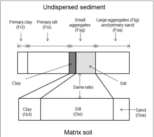
(18) 7. 2.1. Sediment composition by Foster et al. (1985) Foster et al. (1985) developed a set of equations to describe five particle classes in. sediment with differences in density, size, and composition, as a function of the distribution of primary particles in the matrix soil. This distribution of particle size determine the particles’ transportability (ASCE, 1975; Lovell and Rose, 1988a), which is important for applying detachment and transport equations used in erosion models, and for describing chemical transport by sediment (Foster et al., 1985). These equations were derived using data from 24 soils reported in the literature (Alberts et al., 1983; Fertig et al., 1982; Gabriels and Moldenhauer, 1978; Meyer et al., 1980; and Young, 1980) and four from unpublished data from R.A. Young and W.H. Nieibling. The data used to describe the sediment was obtained from sedimentation plots of different lengths instead of using the sediment at the point of detachment. The soils used to build these equations were agricultural soils or of fallow conditions. The five particle classes defined by Foster et al. (1985) were primary clay (Fcl), primary silt (Fsi), small aggregates (Fsg), large aggregates (Flg) and primary sand (Fsa). Small aggregates are composed of clay and silt, and large aggregates of clay, silt and sand. The matrix soil corresponds to the dispersed soil and is formed by clay (Ocl), silt (Osi), and sand (Osa). Thus, the sediment composition was related to the matrix soil texture as shown in Fig. 1..

(19) 8. Figure 1. Composition of the undispersed sediment and matrix soil. The ratio of clay to silt in the small aggregates is assumed to be the same as that in the matrix soil. Adapted from Foster et al. (1985).. A diameter and specific gravity were assigned to each particle class. Fcl represents particles with a diameter < 4 µm, Fsi and Fsg were included in the 4 µm to 63 µm size range, and Fsa and Flg were assigned a diameter > 63 µm. The 4 µm threshold for primary clay particles was defined based on the smallest size reported for the experimental data, and the 63 µm threshold was used because it was a value typically reported and was dictated by the mesh size of available sieves. Only the fraction of primary clay was the obtained directly from experimental data. Small aggregates were estimated assuming that the ratio of silt to clay in small aggregates was the same as in the matrix soil (Fig. 1) and that the silt enrichment in the 4-63 µm sized sediment was primary silt not associated with silt-sized aggregates. The.

(20) 9. primary sand was estimated assuming that the fraction of primary sand in the sediment > 63 µm was the same as the fraction of sand in the matrix soil. The fraction of large aggregates was obtained by difference with the rest of the sediment classes. Once the sediment composition was obtained, the fractions were related to the matrix soil texture. For Fcl and Fsg a direct relationship to Ocl was assumed. For Fsi, it was assumed that the fraction of sediment between 4-63 µm, which includes Fsi and Fsg, was equal to Osi. For Fsa, a direct relationship with Osa and an indirect one with Ocl were assumed. Therefore, the equations obtained by Foster et al. (1985) are shown in Table 1 as Eqs. (1) to (7). The small and large aggregates’ compositions were given by equations (18) to (23) shown in Table 1. The fractions of clay and silt in small aggregates were obtained assuming that the ratio of silt to clay in the small aggregates was the same as in the matrix soil, and the composition of the large aggregates was obtained by difference. The compositions for primary clay, primary silt and primary sand are not shown in Table 1 because they only have clay, silt and sand, respectively. In addition, it was arbitrarily assumed that the clay content in the large aggregates should be at least one half that of the matrix soil for large aggregate stability. When that was not the case, the small aggregate class was recomputed to ensure minimum clay content for the large aggregates..

(21) Table 1. Sediment and aggregate composition according to Foster et al. (1985) and the developed equations for uncultivated and fire-affected soils. Foster et al. (1985). Fcl Fsi Fsg. Fsa Flg. 0.26  Ocl Osi - Fsg 1.8 Ocl 0.45 - 0.6  (Ocl - 0.25) 0.6  Ocl. Ocl  0.25 0.25  Ocl  0.5 Ocl  0.5. Osa (1 - Ocl)5 1 - Fcl - Fsi - Fsg - Fsa. Uncultivated soils Sediment Composition (1) (2) (3) (4) (5) (6) (7). Fire-affected soils. 0.005  Ocl 1 - Fcl - Fsg - Flg - Fsa. (8) (9). 0.009  Ocl 1 - Fcl - Fsg - Flg - Fsa. (13) (14). 1.593  Ocl. (10). 3.146  Ocl. (15). Osa  (1 - Ocl)0.83. (11) (12). Osa  (1 - Ocl)1.30 4.341 Ocl. (16) (17). (24) (25) (26) (27) (28) (29). (Ocl  Fcl  Flg  f, cl, lg)/Fsg 0.421  Osi/Fsg 0 0.638  Ocl/Flg (Osi  Fsi  Fsg  f, si, sg)/Flg (Osa - Fsa)/Flg. (30) (31) (32) (33) (34) (35). 4.248  Ocl Aggregate Composition. f,cl,sg f,si,sg f,sa,sg f,cl,lg f,si,lg f,sa,lg. Ocl/(Ocl Osi) Osi/(Ocl  Osi) 0 (Ocl - Fcl - Fsg  f, cl, sg)/Flg (Osi - Fsi - Fsg  f, si, sg)/Flg (Osa - Fsa)/Flg. (18) (19) (20) (21) (22) (23). (Ocl  Fcl  Flg  f, cl, lg)/Fsg (Osi  Fsi  Flg  f, si, lg)/Fsg 0 0.692  Ocl/Flg 0.612  Osi/Flg (Osa - Fsa)/Flg. 10. Ocl, Osi, Osa: clay, silt and sand in the matrix soil. Fcl, Fsi, Fsg, Fsa, Flg: primary clay, primary silt, small aggregates, primary sand and large aggregates. f,cl,sg, f,si,sg, f,sa,sg: fraction of clay, silt and sand in the small aggregates. f,cl,lg, f,si,lg, f,sa,lg: fractions of clay, silt and sand in the large aggregates. Compositions for the primary clay, primary silt and primary sand are not shown because they only have clay, silt, and sand, respectively..

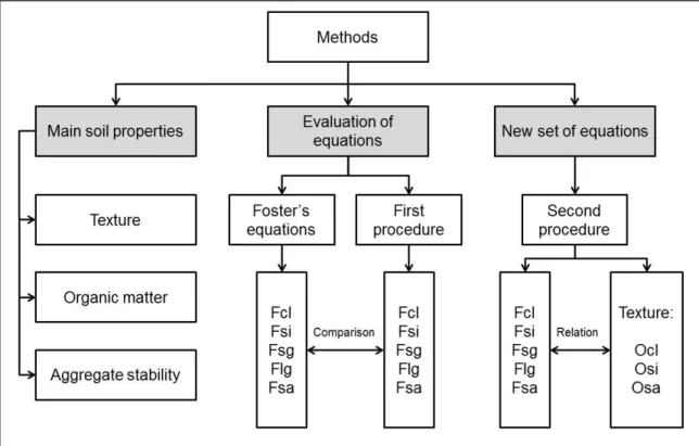
(22) 11. 3. MATERIALS AND METHODS In this section the materials and methods used to describe the sediment. composition of uncultivated and fire-affected soils are presented. Figure 2 shows a diagram with the main analyses performed and the objectives (in grey): describing the properties of the soils samples, evaluating Foster’s equations, and developing a new set of equations for uncultivated and fire-affected soils. To obtain the main soil properties, texture, organic matter content, and aggregate stability analyses were performed. To evaluate Foster’s equations, the fractions of sediment computed with the equations were compared with the fractions measured in the soil samples, and to develop a new set of equations, the fractions of sediment obtained with a second procedure were related to the soil matrix texture.. Figure 2. Main analyses performed to describe the sediment composition in both, uncultivated and fire-affected soils. Grey boxes show the three main objectives..

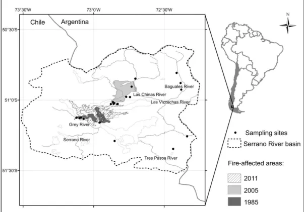
(23) 12. 3.1. Soil samples and study area Soil samples were taken from different soils in the Serrano river basin at the. Chilean Patagonia on a field campaign in December 2012. The site selection considered different soil types, land cover, and the occurrence of fire events. Samples were taken at 23 sites, nine of them affected by at least one of the three major fires registered in the basin. At each site, soils were sampled at 0.2 m depth with a replicate separated approximately 10 - 15 m away. Thus, a total of 46 samples were obtained for laboratory analysis. The Serrano river basin is located in the Chilean Patagonia (Fig. 3) between 50°33’ S and 51°32’ S and between 72°10’ W and 73°34’ W with a total area of 6,673 km2 (Bonilla et al., 2014). It has an irregular topography and the main geomorphologic feature is the Patagonian mountain range which is interrupted by major lacustrine bodies.. Figure 3. Location of the Serrano river basin, sampling sites, and fire-affected areas after the three major fires..

(24) 13. The average annual precipitation in the study area ranges from 200 mm yr-1 on the eastern side to 1,000 mm yr-1 on the western side. The mean annual temperature is approximately 7°C, with a minimum temperature of 3°C in August and a maximum of 13°C in January (DGA-MOP, 1987). The dominant vegetation is the native evergreen forest in the western sector and bushes and peaty scrubland in the cooler areas (Michea et al., 1996). There are nearly no human settlements, except for tourism and hotel facilities. The main four soil types are Luvic Phaeozems (28% of the basin area), Dystric Cambisols (24%), Lithosols (13%), and Eutric Cambisols (10%). The rest of the basin area corresponds to water bodies, rocky areas, glaciers and snow (IUSS working group WRB, 2007). Half of the basin belongs to the Torres del Paine and Bernardo O’Higgins National Parks, with highly sensitive ecosystems. The Torres del Paine National Park is a world biosphere reserve and one of the most important landmarks in Chile (Domínguez et al., 2006). The number of visitors in the park increases the risk of ignition sources (Vidal and Reif, 2011); since 1980, more than 60 fires have been recorded in the park, affecting approximately 48,000 ha, or nearly 20% of the park’s area (Cifuentes, 2013). The three major fires registered in the recent years occurred in 1985, 2005 and 2011.. 3.2. Sample analyses The soil samples were dried at 40°C overnight and sieved (≤ 2 mm). The soil. analyses included organic matter content, soil texture, and aggregate stability. For the sediment composition analysis in different soil fractions, the samples were previously sieved at 53 µm and 250 µm. The organic matter content was determined by oxidation with a mixture of dichromate and sulfuric acid (Nelson and Sommers, 1996). The soil texture was measured by the pipette method (Gee and Bauder, 1986), and the sand, silt and clay contents were defined according to the U.S. Department of Agriculture (USDA) particle-size limits classification (Soil Survey Staff, 1975). The aggregate stability was measured using a wet sieving apparatus (Eijkelkamp, Giesbeek,.

(25) 14. Netherlands), and calculated as the ratio of stable to total aggregates in the 1-2 mm range as presented by Kemper and Rosenau (1986).. 3.3. Sediment composition The sediment composition was measured with two procedures. Both used a. methodology equivalent to the one used by Foster et al. (1985), but with some differences that are explained next. The particle-size limits were defined according to the USDA classification, which is a standard system but different from the definition used by Foster et al. (1985). The USDA classification defines clay-sized particles as < 2 µm, silt-sized particles as between 2 µm to 50 µm, and sand-sized particles as > 50 µm. In Foster’s study, clay-sized particles were < 4 µm, silt-sized particles were between 4 µm to 63 µm, and sand-sized particles were > 63 µm. Unlike the procedure used by Foster et al. (1985), the same soil sample was used to obtain the soil matrix texture and the fractions of the undispersed sediment. Thus, it was possible to obtain the sediment composition at its point of detachment rather than at the end of a hillslope, enabling the implementation of these results on erosion models that generate the detachment and transport for different particle classes of sediment. The first procedure provides an evaluation of Foster’s equations with two sets of soil data: uncultivated and fire-affected soils. It replicates the definition of particle classes used by Foster et al. (1985), where small aggregates are silt-sized, and large aggregates are sand-sized. The second procedure was used to derive a new set of equations for both sets of soil data. In this last procedure, the small and large aggregates were defined as sand-sized particles, with a diameter between 50 µm to 250 µm for the small aggregates, and > 250 µm for the large aggregates. The particles were re-defined in the second procedure because of the poor results obtained with the first one. With the first procedure, the sediment composition showed that the fraction of sediment < 50 µm, which contains the primary clay, primary silt, and small aggregates, was extremely small, and the sediment was highly clustered in aggregates > 50 µm. Thus, to better represent the composition of these soils, the aggregates were defined as larger particles..

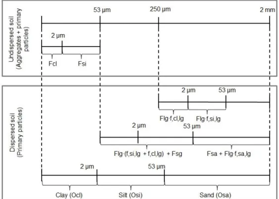
(26) 15. The threshold of 250 µm between the small and large aggregates was defined based on previous studies (Márquez et al., 2004; Mataix-Solera et al., 2011; Tisdall and Oades, 1982). In both procedures, small aggregates were assumed to have only clay and silt particles, and large aggregates to have clay, silt, and sand particles. This composition was also assumed by Foster et al. (1985) as shown in Table 1, where the fraction of sand in small aggregates (f,sa,sg) was zero.. 3.3.1. First procedure. A combination of two techniques, dry sieving and pipette extraction (Gee and Bauder, 1986), which were also used by Foster et al. (1985), was implemented to measure the sediment particle-size and the five particle classes. It is important to notice that even though both are standard techniques, sieving evaluates particle cross section whereas pipetting is based on particle fall velocity according to Stokes’ law. The samples were dried at 40°C overnight and sieved to 2 mm and 53 µm. Sediment with particle size > 53 µm, which contains primary sand and large aggregates, was dispersed and measured with pipette withdrawals. With this measurement, the silt and clay particles forming the large aggregates and the sand in both the primary sand and sand in the large aggregates were obtained. The sediment fraction with particle size < 53 µm was also measured with pipette withdrawals but without previous dispersion to avoid dissolving the small aggregates. Thus, the clay measurements through pipette withdrawals only correspond to primary clay (Fcl). Another sample of soil (< 2 mm) was measured. with. the. pipette. technique,. but. with. dispersant. agent. (Sodium. Hexametaphosphate) to directly obtain the Ocl, Osi, and Osa in the matrix soil. Figure 4 summarizes the three pipette texture analyses and the obtained fractions..

(27) 16. Figure 4. First procedure used to evaluate the sediment composition. Three pipette analyses were required to obtain the texture from different fractions of the undispersed soil. Fsi: primary silt; Fsg: small aggregates; Fcl: primary clay; Fsa: primary sand; f,sa,lg, f,si,lg, f,cl,lg: fraction of sand, silt and clay in large aggregates respectively.. As shown in Figure 4, the only sediment fraction directly measured was Fcl, and two assumptions were made for the other four particle classes. The silt to clay ratio in Fsg was assumed to be the same as that in the matrix soil, and Fsa was estimated assuming that the fraction of sand in the sediment > 53 µm was the same as that in the matrix soil as well. Both assumptions were also made in the study by Foster et al. (1985), so the results are comparable. Flg was obtained by difference because the sum of fractions for all particle classes must be equal to one. Some difficulties occurred when trying to estimate Fsg and Fsi because the fraction of sediment < 53 µm was too small. In certain cases, the fraction of primary clay (Fcl) was equal to the total clay in the fraction of sediment < 53 µm, which led to the lack of clay in small aggregates and consequently to the absence of Fsg. In addition, when clay was found in Fsg, the computed fraction of silt in small aggregates led to an.

(28) 17. overestimation of Fsg. Thus, the Fsg had to be adjusted to a maximum computed as the difference between the fraction of sediment < 53 µm and Fcl. This meant that the fraction of primary silt (Fsi) in those cases was zero. Once the sediment fractions were obtained, they were compared to the fractions computed with Foster’s equations to evaluate them on uncultivated and fire-affected soils.. 3.3.2. Second procedure. The same five particle classes were used in this procedure, but defining large aggregates as particles with diameters > 250 µm and small aggregates as particles with a diameter between 53 and 250 µm. The same preparation used in the first procedure was applied (drying at 40°C overnight and sieved to 2 mm) with the same techniques of sieving and pipette withdrawals, but with an additional pipette analysis for the fraction > 250 µm as shown in Fig. 5. Because the pipette analyses were made on different soil subsamples, the measured clay, silt or sand in the fraction of sediment > 250 µm was similar or even larger than the clay, silt or sand measured in the entire sample (< 2 mm) in some cases. When this happened, an additional pipette analysis was performed to the fraction of sediment < 250 µm. Thus, Ocl, Osi, and Osa were obtained as a weighted sum of the clay, silt and sand of each fraction (smaller and larger than 250 µm). This explains why the total clay, silt, and sand of the matrix soil are not equal in both procedures..

(29) 18. Figure 5. Second procedure used to evaluate the sediment composition. Four pipette analyses were required to obtain the texture from different fractions of the undispersed soil. Fsi: primary silt; Fsg: small aggregates; Fcl: primary clay; Fsa: primary sand; f,sa,lg, f,si,lg, f,cl,lg: fraction of sand, silt and clay in large aggregates, respectively.. In this procedure, Fcl and Fsi were measured directly, and in total they correspond to the fraction of sediment < 53 µm (Fig. 5). An assumption was only used to estimate Fsa, the same one used in the first procedure. The rest of the sediment fractions were obtained directly from the pipette analysis. As shown in Fig. 5, the pipette analysis made to the fraction > 250 µm provided the clay and silt in large aggregates, and the analysis with the fraction > 53 µm provided the clay and silt in both the large and small aggregates. Flg was obtained by difference with the rest of the sediment fractions. To generate the new set of equations relating the soil matrix texture and the fractions of sediment, Fcl, Fsg and Flg were related to Ocl as clay usually acts as a bonding agent in soil aggregation (Young, 1980). As in Foster’s study, Fsa was associated with Ocl and Osa, and Fsi was obtained by difference. To obtain the.

(30) 19. aggregates’ compositions, the fraction of clay in the large aggregates (f,cl,lg) was related to Ocl for the uncultivated and fire-affected soils, the fraction of silt in the large aggregates (f,si,lg) was associated with Osi for the uncultivated soils, and the fraction of silt in the small aggregates (f,si,sg) was related to Osi for the fire-affected soils. The rest of the compositions were obtained by difference. The regression equations for both sets of soil samples were compared using Student’s t test with a level of significance of P  0.05. The analysis was performed according to Zar (2010). In that way, it was possible to determine if the soils affected by fire behaved differently than uncultivated soils..

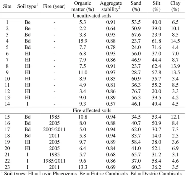
(31) 20. 4. RESULTS AND DISCUSSION The main soil properties obtained through laboratory analyses are summarized in. Table 2. The organic matter (OM) content showed a mean value of 7.4% for the uncultivated soil samples ranging from 2.2% to 15.9% with a standard deviation of s = 3.5%. In fire-affected soils the OM content was slightly higher (8.3%) ranging from 5.0% to 13.3% and a standard deviation of 2.8%. The aggregate stability showed a mean value of 0.85, very close to the uncultivated (with a mean of 0.84 and s = 0.11) and fireaffected soil samples (with a mean of 0.85 and s = 0.10). Almost half of the soils had a sandy loam texture, and the rest of the samples were silt loam, loam and loamy sand. Because of the content of organic matter and aggregate stability, these soils can be considered rich in OM and with very stable aggregates according to the classification of Mataix-Solera et al. (2010), which is typical of soils in natural conditions (Brady and Weil, 2002). The difference in OM content between the uncultivated and fire-affected soils was not uncommon. Fire-affected soils can show an increment in the OM and nutrient contents due to the deposition of dry leaves and charred plant materials (González-Pérez et al., 2004). In addition, aggregate stability can increase after a fire depending on many factors such as fire severity and intensity, time after the fire, and composition of the aggregates (Mataix-Solera et al., 2011). However, this study was not intended to evaluate the effects of fire on soil properties as samples before and after the occurrence of a fire event were not compared. More detail about those effects in the study area was reported by Bonilla et al. (2014)..

(32) 21. Table 2. Main properties of the soil samples used in the study. Organic Aggregate Sand Silt Clay 2 matter (%) stability (%) (%) (%) Uncultivated soils 1 Be 5.3 0.91 53.5 40.0 6.5 2 Be 2.2 0.64 50.9 39.0 10.1 3 Bd 3.8 0.93 67.6 23.9 8.5 Bd 4 15.9 0.88 23.7 61.8 14.5 Bd 5 7.7 0.78 24.0 71.6 4.4 6 Hl 6.8 0.93 56.0 37.0 7.0 Hl 7 7.9 0.86 46.9 44.4 8.7 Hl 8 7.5 0.91 23.7 62.4 13.9 Hl 9 11.0 0.97 28.7 57.8 13.5 Hl 10 8.9 0.85 60.9 35.7 3.4 Hl 11 4.9 0.81 36.3 55.2 8.5 Hl 12 3.4 0.86 76.7 20.0 3.3 Hl 13 9.0 0.89 56.3 39.5 4.2 14 I 9.3 0.57 46.1 49.4 4.5 Fire-affected soils 15 Bd 1985 10.8 0.94 34.5 53.4 12.1 Bd 16 2005 8.0 0.88 40.7 50.9 8.4 Bd 17 2005/2011 5.0 0.94 62.0 30.7 7.3 Bd 18 2011 5.8 0.94 83.7 14.0 2.3 19 Hl 2005 9.7 0.89 58.4 38.0 3.6 20 Hl 2005 6.4 0.84 41.0 52.1 6.9 21 I 1985 5.7 0.68 65.7 31.2 3.1 22 I 1985/2011 9.6 0.86 37.0 58.4 4.6 23 I 2011 13.3 0.69 60.3 36.2 3.5 1 Soil types: Hl = Luvic Phaeozems, Be = Eutric Cambisols, Bd = Dystric Cambisols, I = Lithosols. 2 Calculated as the ratio of stable to total aggregates. Site. Soil type1 Fire (year).

(33) 22. 4.1. Equations based on agricultural soils The fractions of sediment measured with the first procedure are shown in Table 3.. On average, Fcl represents less than 0.04% of the sediment composition for the uncultivated soils, with a maximum of 0.08%. This is explained because of the small amount of clay in the fraction of sediment < 53 µm and because that fraction was also small. Less than 5% of the undispersed sediment was < 53 µm, ranging from 0.4% to 12.3%. This meant that there were almost no free fine particles in the sediment, which includes primary clay, primary silt and, for the first procedure, small aggregates as defined by Foster et al. (1985). The results were similar for the fire-affected soils, with Fcl approximately 0.05% and 5.4% for the fraction of sediment < 53 µm. Because the fraction of sediment < 53 µm was very small, the estimated Fsi and Fsg with the first procedure were zero in many cases. This happened because the first procedure followed the same assumption used by Foster et al. (1985), that is, that small aggregates were assumed to have a size < 53 µm. It can be seen in Table 3 that this occurred for both sets of samples (uncultivated and fire-affected). The sediment fractions obtained with the first procedure (Table 3) were used to evaluate Eqs. (1) to (7)..

(34) Table 3. Composition of the matrix soil and sediment samples from the study area. Values separated by "/" correspond to the percentages obtained with the first and second procedure, respectively. Site. Ocl. Osi. Osa. 23. Fcl Fsi Fsg* Flg* Fsa Uncultivated soils 1 6.8 / 6.3 39.3 / 38.8 53.9 / 54.9 0.08 / 0.08 11.8 / 11.8 0.0 / 2.6 40.6 / 37.1 47.5 / 48.4 2 8.8 / 10.1 17.6 / 38.8 73.6 / 51.2 0.06 / 0.06 0.0 / 3.5 3.5 / 17.2 25.4 / 29.9 71.0 / 49.3 3 10.1 / 4.3 41.7 / 14.0 48.2 / 81.8 0.02 / 0.02 1.9 / 1.9 0.0 / 7.1 50.8 / 10.8 47.2 / 80.2 4 14.5 / 13.2 57.2 / 55.6 28.3 / 31.3 0.03 / 0.03 0.0 / 3.2 3.2 / 16.4 69.4 / 50.1 27.4 / 30.3 5 4.4 / 3.0 58.3 / 40.1 37.3 / 56.9 0.00 / 0.00 0.0 / 0.4 0.4 / 6.3 62.4 / 36.6 37.2 / 56.7 6 6.9 / 7.0 46.5 / 37.6 46.5 / 55.4 0.08 / 0.08 8.0 / 11.0 3.0 / 15.7 47.5 / 23.9 41.3 / 49.3 7 8.7 / 8.7 45.1 / 44.5 46.1 / 46.7 0.07 / 0.07 4.3 / 12.2 7.9 / 24.5 47.2 / 22.2 40.5 / 41.0 8 13.6 / 10.8 65.9 / 57.5 20.5 / 31.7 0.03 / 0.03 0.0 / 1.4 1.4 / 4.6 78.4 / 62.7 20.2 / 31.3 9 13.9 / 13.3 59.2 / 56.5 26.9 / 30.3 0.07 / 0.07 3.1 / 3.1 0.0 / 8.0 70.8 / 59.6 26.0 / 29.3 10 4.7 / 3.3 34.0 / 35.4 61.3 / 61.3 0.01 / 0.01 1.0 / 1.0 0.0 / 21.6 38.3 / 16.7 60.6 / 60.7 11 6.7 / 7.4 53.7 / 47.2 39.6 / 45.3 0.01 / 0.01 0.0 / 2.4 2.4 / 19.9 58.9 / 33.4 38.7 / 44.2 12 9.5 / 3.2 57.1 / 19.5 33.4 / 77.4 0.03 / 0.03 4.2 / 4.2 0.0 / 9.6 63.8 / 12.0 32.0 / 74.1 13 5.8 / 4.2 47.0 / 39.3 47.2 / 56.5 0.03 / 0.03 4.3 / 4.3 0.0 / 19.3 50.5 / 22.3 45.2 / 54.1 14 4.5 / 4.5 43.3 / 49.5 52.2 / 46.0 0.03 / 0.03 7.2 / 9.3 2.1 / 27.8 43.4 / 21.1 47.3 / 41.7 Fire-affected soils 15 10.2 / 4.3 29.2 / 29.5 60.6 / 66.2 0.11 / 0.11 0.0 / 5.7 5.7 / 10.2 37.1 / 21.6 57.1 / 62.4 16 8.5 / 5.0 43.0 / 30.0 48.6 / 65.0 0.03 / 0.03 0.0 / 4.5 4.5 / 17.0 49.1 / 16.4 46.4 / 62.0 17 7.3 / 8.1 22.4 / 26.9 70.2 / 65.1 0.02 / 0.02 0.0 / 2.5 2.5 / 6.6 29.0 / 27.5 68.5 / 63.4 18 2.3 / 2.3 18.2 / 14.0 79.5 / 83.7 0.03 / 0.03 1.2 / 3.3 2.0 / 5.4 19.8 / 10.4 76.9 / 81.0 19 7.5 / 6.5 55.6 / 50.5 36.9 / 43.1 0.07 / 0.07 4.4 / 4.4 0.0 / 23.8 60.3 / 30.6 35.2 / 41.1 20 6.7 / 7.0 41.9 / 52.4 51.5 / 40.6 0.03 / 0.03 0.0 / 3.3 3.3 / 30.3 46.9 / 27.1 49.7 / 39.2 21 6.4 / 3.1 45.4 / 34.3 48.2 / 62.6 0.03 / 0.03 5.8 / 5.8 0.0 / 17.1 48.8 / 18.1 45.4 / 58.9 22 4.6 / 4.4 46.0 / 56.8 49.4 / 38.8 0.13 / 0.13 2.9 / 14.1 11.2 / 28.3 43.5 / 24.2 42.4 / 33.3 23 6.9 / 3.5 64.3 / 36.4 28.9 / 60.1 0.01 / 0.01 4.3 / 4.3 0.0 / 10.2 68.0 / 27.9 27.6 / 57.5 *Fractions of small and large aggregates are not directly comparable as they were defined differently in both procedures..

(35) 24. The values for the uncultivated soils were plotted in Fig. 6. With the exception of Fsa, the coefficient of determination (r2) between the predicted and measured values was less than 0.05 and the Nash-Sutcliffe efficiency (N-S) was negative for all the fractions. The Fsa showed a good fit with an r2 of 0.88 but not a high N-S (0.01) because the values were under-predicted. Fig. 6 shows that Fcl, Fsi, and Fsg were over-predicted when using Foster’s equations, while Flg and Fsa were under-predicted. The results showed that most of the sediment in uncultivated soils was in the form of large aggregates, and primary clay and silt were not found in the sediment. It is important to note that the thresholds used to define the particle sizes in this procedure were defined according to the USDA classification, which is slightly different from the limits used by Foster et al. (1985). However, this difference is not large enough to explain the lack of fit with Foster’s equations. The exponent in Eq. (6) from Table 1 was modified to fit the measured values of Fsa. The exponent was calculated by rearranging Eq. (6) and computing the mean exponent from the fractions obtained for the studied soils. This resulted in an exponent of 0.71 instead of 5. The adjusted equation shows a better fit (Fig 6-f), with r2 and N-S of 0.97. The smaller exponent in Eq. (6) suggests that Fsa depends mainly on Osa but not on Ocl. This means that most of the sand in the sediment is found as primary sand and not aggregated with clay or silt. The results showed that on average, the fraction of sand in the large aggregates was 5.3%, ranging from 0.3% to 15.7% for the uncultivated soils, which demonstrates that a small fraction of the large aggregates has sand. Using Eq. (23), the fraction of sand in large aggregates (f,sa,lg) was estimated as 69.8%, ranging from 51.3% to 80.7%, which is larger than the measured values. Using the adjusted values for Fsa and re-computing Eq. (23) resulted in smaller estimates of the fraction of sand in large aggregates (f,sa,lg), ranging from 9.7% to 13.8% with a mean of 11.8%..

(36) 25. Figure 6. Comparison between the sediment fractions obtained with the first procedure and with the equations developed by Foster et al. (1985) for the uncultivated soils. Dashed lines represent linear regressions and dotted lines represent the 1:1 line. The r2 values correspond to the best fit (linear regression)..

(37) 26. Fire-affected soils were also compared and similar results were observed. The fractions measured with the first procedure are also shown in Table 3. When using Foster’s equations, the values of Fcl, Fsi, and Fsg were over-predicted, while Flg and Fsa were under-predicted. The plotted values for the fire-affected soils are not shown; however, with the exception of Fsa, the N-S efficiencies were negative and the r2 were very low. For Fcl, Fsi, Fsg, Flg, and Fsa, the N-S efficiencies were -1930, -177, -8.05, 3.60, and 0.16, respectively. The r2 were 0.01, 0.53, 0.00, 0.03, and 0.84, respectively. The only difference was found for Fsi, where the r 2 was better than for the uncultivated soils. Adjusting the exponent in Eq. (6) resulted in a value of 0.97 and in an improvement of the prediction with an r2 and N-S efficiency of 0.98. In this case, the fraction of sand in the large aggregates (f,sa,lg) was also small, with a mean value of 7.1% compared to the 74.5% computed with Eq. (23). The only adjustment performed to fit the data was applied to Eq. (6) because there was almost no sediment < 53 µm. This is because three of the sediments’ fractions (Fcl, Fsi, and Fsg) were almost not found in the sediment, and the sediment was mostly aggregated in particles > 53 µm. Thus, most of the effort was to improve the precision for predicting sediment particles > 53 µm and not much for particles < 53 µm. With that purpose, the particle threshold was changed, and the second procedure was used to fit new equations to predict the sediment and aggregate’s composition for the uncultivated and fire-affected soils. The fractions obtained with the second procedure are also shown in Table 3.. 4.2. New equations for the uncultivated and fire-affected soils The fractions obtained with the second procedure were different from those. obtained with the first procedure, except for the fractions of primary clay (Fcl), which were the same in both because they were measured directly. For the uncultivated soil samples, Fsi was 1.7% larger than the value obtained with the first procedure because the small aggregates were no longer associated with the same fraction of primary silt. The same condition was observed with the Fsg, 14.3% compared to 1.7% because the.

(38) 27. small aggregates were larger in the second procedure and thus included a larger portion of sediment. The opposite was observed with Flg, with 31.3% compared to 53.4%. Fsa was 49.3% compared to 41.6% with the first procedure. For the fire-affected soil samples, the fractions with the second procedure showed means of 0.05%, 5.3%, 16.5%, 22.6%, and 55.4% for Fcl, Fsi, Fsg, Flg, and Fsa, respectively, while with the first procedure, the same fractions were 0.05%, 2.1%, 3.2%, 44.7%, and 49.9%. The sediment fractions were related to the soil texture and the fitted equations are shown in Table 1, namely, Eqs. (8) to (12) and (13) to (17) for the uncultivated and fireaffected soil samples, respectively. Compared to Foster’s equations, the computed fractions for primary clay (Fcl) were smaller for the same amount of clay in the matrix soil (Ocl). This happened because in these soils almost no primary clay was found in the sediment, with most in the small and large aggregates. Comparing Eq. (6) with Eqs. (11) and (16), which predict the fraction of primary sand, the exponent is smaller in Eqs. (11) and (16). This means that most of the sand in these soils is found as primary sand and not aggregated. The fit of equations (8), (10), (11), and (12) is shown in Figure 7. The regression between Fcl and Ocl had an r2 = 0.21, and 0.01 between Fsg and Ocl. However, the regression for Flg was better (r2 = 0.60). For the uncultivated soil samples, the relationship between the estimated and predicted (with Eq. (11)) fractions of primary sand showed an r2 = 0.98 and an N-S = 0.98..

(39) 28. Figure 7. Relationships between the sediment fractions obtained with the second procedure and the clay content (a, b, and c) and between predicted and estimated primary sand (d) for the uncultivated soil samples. Dashed lines represent the linear regression and solid lines represent the best linear fit with intercept zero. The r2 values correspond to the best fit (linear regression).. A robust Fsa and Flg estimation is particularly important in the uncultivated soil samples as they represent approximately 80% of the sediment composition. The rest of the fractions were not predicted well, but they represent less than 20% of the sediment. The scatter in Fig. 7 for the primary clay (Fig. 7-a) and small aggregates (Fig. 7-b) show that those fractions are affected by other factors beyond the clay content in the matrix.

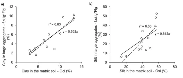
(40) 29. soil, which could be the type of organic matter present in the soil or any other factor that could not be evaluated with this analysis. The fit for the equations derived for the fire-affected soil samples is not shown, but it was similar to that for the uncultivated soils, with low r 2 for Fcl (0.01) and Fsg (0.10) but larger values for Flg (0.47) and Fsa (0.97). In this case, Fsa and Flg also represent most of the sediment composition, 78.1% on average. The equations derived in this study are not necessarily valid for soils with Ocl values larger than 20%. These equations were fitted for soil samples where the maximum value for Ocl was 13.3% and 8.1% for the uncultivated and fire-affected soil samples, respectively. Therefore, the use of these equations for soils beyond that limit has a degree of uncertainty that was not evaluated in this study. The aggregate composition was also adjusted for these soils as shown in Eqs. (24) to (29) for the uncultivated soils, and Eqs. (30) to (35) for the fire-affected soils. The regression for Eqs. (27) and (28) showed an r2 of 0.83 and 0.63, respectively (Fig. 8). For the fire-affected soils, the fraction of silt in the small aggregates (f,si,sg) showed a better fit with Osi than the fraction of silt in the large aggregates (f,si,lg). Thus, Eq. (31) was not obtained by difference but calculated directly, and Eq. (34) was obtained by difference, as opposed to the equations presented for the uncultivated soils. Equations (31) and (33) showed an r2 of 0.84 and 0.78, respectively..

(41) 30. Figure 8. Relationship between the clay content in the large aggregates (as percentage of the total sediment) and clay in the matrix soil (a) and between the silt in the large aggregates (as percentage of the total sediment) and the silt in the matrix soil (b) for the uncultivated soil samples. Dashed lines represent linear regression (r2 shown) and solid lines represent the best linear fit with intercept zero.. The regression between Fcl, Fsg, and Flg with Ocl were compared for the uncultivated and fire-affected soils. The results showed no statistically significant difference between them. The regressions for the aggregate composition equations were also compared, and no differences were found. However, the fitted equations were different and the results are presented separately for the uncultivated and fire-affected soils to obtain a better and more specific soil characterization..

(42) 31. 5. CONCLUSIONS All the soil samples evaluated in this study showed high OM contents and. aggregate stability and undispersed soil fractions that were significantly different from those predicted with Foster’s equations. Those equations, originally developed from cultivated soils, proved not to be suitable for predicting the sediment composition in uncultivated and fire-affected soils. The equations over-predicted the fractions of primary clay, primary silt, and small aggregates and under-predicted the fractions of large aggregates and primary sand in both fire-affected and uncultivated soil samples. With the exception of primary sand, which was not found in the aggregates in these soils, the obtained and computed fractions showed a negative N-S efficiency and low r2 (< 0.05 for uncultivated soils and < 0.53 for fire-affected soils) in all the sediment fractions. The fraction of primary sand showed a good fit for both the uncultivated and fireaffected soils, with an r2 of 0.88 and 0.84, respectively, but a low N-S of 0.01 and 0.16. Once adjusted, the equation for primary sand provided a much better prediction, with an r2 and N-S efficiency over 0.97 for both the uncultivated and fire-affected soil samples. The equation was fitted by recalculating the exponent of the equation for primary sand, which resulted in a smaller value. This meant that the sand in the sediment for these soils was mainly free and not aggregated with clay or silt. The rest of the equations were not adjusted because the soil particles were mostly grouped in large aggregates (> 250 µm). Additionally, the fine particles (< 53 µm) in these soils represented less than 5%, including primary clay, primary silt and small aggregates as defined by Foster et al. (1985). Once the limits for the small (between 50 µm and 250 µm) and large aggregates (> 250 µm) were re-defined, the new equations for the uncultivated and fire-affected soils provided considerably better estimates of the fractions of large aggregates, primary sand, and aggregate composition. However, the relationship between the primary clay and small aggregates with clay in the matrix soil was poor, but these fractions represented less than 20% of the sediment..

(43) 32. Overall, the results of this study demonstrate that the sediment composition is significantly different between uncultivated and agricultural soils. The main difference between them was related to the particles’ aggregation, as the uncultivated soils were mostly formed by large aggregates (> 250 µm) with high stability and organic matter content. In addition, the sand in sediments was mainly found as free particles and not in the aggregates. Finally, the equations developed in this study provide more reliable sediment composition estimates when predicting soil erosion on uncultivated or fire affected soils, increasing the understanding of nonpoint source pollution processes when planning soil and water conservation practices..

(44) 33. REFERENCES Aksoy, H. and Kavvas, M.L. (2005). A review of hillslope and watershed scale erosion and sediment transport models. Catena, 64(2-3), 247–271. Alberts, E.E., Wendt, R.C. and Piest, R.F. (1983). Physical and chemical properties of eroded soil aggregated. Transactions of the ASAE, 26(2), 465-471. American Society of Civil Engineers. (1975). Sedimentation Engineering, ASCE Manuals and Reports on Engineering Practice, No. 54, V.A. Vanoni (Ed.), ASCE, New York. Angers, D.A. and Caron, J. (1998). Plant-induced changes in soil structure: processes and feedbacks. Biogeochemistry, 42(1), 55–72. Beasley, D.B., Huggins, L.F. and Monke, E.J. (1980). ANSWERS — a model for watershed planning. Trans. ASAE, 23(4), 938–944. Bonilla, C.A., Norman, J.M. and Molling, C.C. (2007). Water erosion estimation in topographically complex landscapes: Model description and first verifications. Soil Science Society of America Journal, 71(5), 1524–1537. Bonilla, C.A., Pastén, P.A., Pizarro, G.E., González, V.I., Carkovic, A.B. and Céspedes, R.A. (2014). Forest fires and soil erosion effects on soil organic carbon in the Serrano river basin (Chilean Patagonia). In A.E. Hartemink, K. McSweeney (Eds.), Soil Carbon. Progress in soil science (pp. 229-237). Switzerland: Springer International Publishing. Brady, N.C. and Weil, R.R. (2002). The nature and properties of soils. (13th ed.). Upper Saddle River, N.J.: Pearson/Prentice Hall. Bridges, E.M. and Oldeman, L.R. (1999). Global assessment of human-induced soil degradation. Arid Soil Research and Rehabilitation, 13(4), 319–325..

(45) 34. Certini, G., 2005. Effects of fire on properties of forest soils: a review. Oecologia 143, 1–10. Cifuentes, R. (2013). Mega wildfire in the world biosphere reserve (UNESCO), Torres del Paine National Park, Patagonia – Chile 2012: Work experience in extreme behavior conditions in the context of global warming. In proceedings of the fourth international symposium on fire economics, planning, and policy: climate change and wildfires. Gen. Tech. Rep. PSW-GTR-245 (English). Albany, CA: U.S. Department of Agriculture, Forest Service, Pacific Southwest Research Station. 405 pp. De Ploey, J. and Poesen, J. (1985). Aggregate stability, runoff generation and interrill erosion, in: Richards, K.S., Arnett, R.R., Ellis, S. (Eds.), Geomorphology and Soils. George Allen & Unwin, London, pp. 99–120. De Roo, A.P.J., Wesseling, C.G. and Ritsema, C.J. (1996). LISEM: A single-event physically based hydrological and soil erosion model for drainage basins. I: Theory, input and output. Hydrological Processes, 10, 1107–1117. DeBano, L.F. (2000). The role of fire and soil heating on water repellency in wildland environments: a review. Journal of Hydrology, 231-232, 195–206. DGA-MOP. (1987). Balance Hídrico de Chile. Ministerio de Obras Públicas, Santiago, Chile. Domínguez, E., Arve, E., Clodomiro, M. and Pauchard, A. (2006). Plantas introducidas en el Parque Nacional Torres del Paine, Chile. Guayana Bot. 63(2), 131–141. (In Spanish) Fertig, L.H., Monke, E.J. and Foster, G.R. (1982). Characterization of eroded soil particles from interrill áreas. ASAE paper No. 82-2038, ASAE. St. Joseph, MI. 49085.

(46) 35. Foster, G.R., Young, R.A. and Neibling, W.H. (1985). Sediment composition for nonpoint source pollution analyses. Transactions of the ASAE, 28(1), 133-139, 146. Gabriels, D. and Moldenhauer, W.C. (1978). Size distribution of eroded material from simulated rainfall: effect over a range of texture. Soil Science Society of America Journal, 42(6), 954-958. Gee, G.W. and Bauder, J.W. (1986). Particle-size analysis. In A. Klute (Ed.), Methods of Soil Analysis, Part 1. Physical and Mineralogical Methods (pp. 383-411). Madison, WI, USA: American Society of Agronomy-Soil Science Society of America. González-Pérez, J.A., González-Vila, F.J., Almendros, G. and Knicker, H. (2004). The effect of fire on soil organic matter: a review. Environment International, 30, 855–870. IUSS Working Group WRB. (2007). World Reference Base for Soil Resources 2006, first update 2007. World Soil Resources Reports No. 103. FAO, Rome. Kemper, W.D. and Rosenau, R.C. (1986). Aggregate stability and size distribution. In A. Klute (Ed.), Methods of Soil Analysis, Part 1. Physical and Mineralogical Methods (pp. 425-442). Madison, WI, USA: American Society of Agronomy-Soil Science Society of America. Knicker, H. (2007). How does fire affect the nature and stability of soil organic nitrogen and carbon? A review. Biogeochemistry, 85, 91–118. Kuznetsov, M.S., Gendugov, V.M., Khalilov, M.S. and Ivanuta, A.A. (1998). An equation of soil detachment by flow. Soil & Tillage Research, 46, 97–102. Lal, R. (2001). Soil degradation by erosion. Land Degradation & Development, 12(6), 519–539..

(47) 36. Le Bissonnais, Y. and Arrouyais, D. (1997). Aggregate stability and assessment of soil crustability and erodibility: II. Application to humic loamy soils with various organic carbon contents. Eur. J. Soil Sci., 48(1), 39-48. Lovell, C. J. and Rose, C.W. (1988a). Measurement of soil aggregate settling velocities. I. A modified bottom withdrawal tube method. Aust. J. Soil Res., 26, 55–71. Lovell, C.J. and Rose, C.W. (1988b). Measurement of soil aggregate settling velocities. II. Sensitivity to sample moisture content and implications for studies of structural stability. Aust. J. Soil Res., 26, 73–85. Márquez, C.O., Garcia, V.J., Cambardella, C.A., Schultz, R.C. and Isenhart, T.M. (2004). Aggregate-size stability distribution and soil stability. Soil Science Society of America Journal, 68, 725-735. Mataix-Solera, J., Benito, E., Andreu, V., Cerdà, A., Llovet, J., Úbeda, X., Martí, C., Varela, E., Gimeno, E., Arcenegui, V., Rubio, J.L., Campo, J., García-Orenes, F. and Badía, D. (2010). ¿Cómo estudiar la estabilidad de agregados en suelos afectados por incendios? Métodos e interpretación de resultados. In A. Cerdà, A. Jordán, A. (Eds.), Actualización en métodos y técnicas para el estudio de suelos afectados por incendios forestales (pp.109-144). Valencia, Spain: Càtedra de Divulgació de la Ciència. Universitat de València. FUEGORED 2010. (In Spanish) Mataix-Solera, J., Cerdà, A., Arcenegui, V., Jordán, A. and Zavala, L.M. (2011). Fire effects on soil aggregation: A review. Earth-Science Reviews, 109(1-2), 44–60. Merritt, W.S., Letcher, R.A. and Jakeman, A.J. (2003). A review of erosion and sediment transport models. Environmental Modelling & Software, 18(8-9), 761–799. Meyer, L.D., Harmon, W.C. and McDowell, L.L. (1980). Sediment sized eroded from crop row sideslopes. Transactions of the ASAE, 23(4), 891-898..

(48) 37. Michea, G., Cunazza, C., Ivanovich, J., Linnebrink, J., Cifuentes, R., Fernández, V., Zambrano, N. and Contreras, J. (1996). Plan de Manejo Reserva Nacional Magallanes. Chile. Corporación Nacional Forestal, Ministerio de Agricultura, Chile. (In Spanish) Morgan, R.P.C. and Quinton, J.N. (2001). Erosion modelling. In W.W. Doe, R.S. Harmon (Eds.), Landscape Erosion and Erosion Modelling (pp.117-139). New York, USA: Kluwer Academic Press. Morgan, R.P.C., Quinton, J.N., Smith, R.E., Govers, G., Poese, J.W.A., Auerswald, K., Chisci, G., Torri, D. and Styczen, M.E. (1998). The European soil erosion models (EUROSEM): a dynamic approach for predicting sediment transport from fields and small catchments. Earth Surf. Processes Landf., 23(6), 527–544. Navarro, R.M., Hayas, A., García-Ferrer, A., Hernández, R., Duhalde, P. and González, L. (2008). Characteristics of areas affected by fire in 2005 at Parque Nacional de Torres del Paine (Chile) as assessed from multispectral images. Revista Chilena de Historia Natural, 81, 95-110. Nearing, M.A., Foster, G.R., Lane, L.J. and Finkner, S.C. (1989). A process-based soil erosion model for USDA-water erosion prediction project technology. Transactions of the ASAE, 32(5), 1587–1593 Neary, D.G., Klopatek, C.C., DeBano, L.F. and Ffolliott, P.F. (1999). Fire effects on belowground sustainability: a review and synthesis. Forest Ecology and Management, 122(1-2), 51–71. Nelson D.W. and Sommers, L.E. (1996). Total carbon, organic carbon, and organic matter. In D.L. Sparks, A.L. Page, P.A. Helmke, R.H. Loeppert, P.N. Soltanpour, M.A. Tabatabai, C.T. Johnston, M.E. Sumner (Eds.), Methods of soil analysis, Part 3: Chemical methods (pp. 961-1010). Madison, WI: Soil Science Society of America, Inc., American Society of Agronomy, Inc..

(49) 38. Oldeman, L.R. (1992). Global Extent of Soil Degradation. Bi-Annual Report 1991-1992. Wageningen: World Soil Information ISRIC. Pimentel, D., Harvey, C., Resosudarmo, P., Sinclair, K., Kurz, D., McNair, M., Crist, S., Shpritz, L., Fitton, L., Saffouri, R. and Blair, R. (1995). Environmental and economic costs of soil erosion and conservation benefits. Science, 267(5201), 1117–1123. Renard, K.G., Foster, G.R., Weesies, G.A., McCool, D.K. and Yoder, D.C. (1997). Predicting soil erosion by water: a guide to conservation planning with the revised universal soil loss equation (RUSLE). Agriculture Handbook, vol. 703. US Department of Agriculture, Washington DC, 384 pp. Sander, G.C., Zheng, T., Heng, P., Zhong, Y. and Barry, D.A. (2011). Sustainable soil and water resources: Modelling soil erosion and its impact on the environment, MODSIM 2011-19th International Congress on Modelling and Simulation - Sustaining Our Future: Understanding and Living with Uncertainty, pp. 45–56, Perth, Western Australia, Australia, 12–16 December. Smith, R.E., Goodrich, D.C. and Quinton, J.N. (1995). Dynamic, distributed simulation of watershed erosion: the KINEROS2 and EUROSEM models. Journal of Soil and Water Conservation, 50(5), 517–520. Soil Science Society of America (SSSA). (2008). Glossary of soil science terms. Retrieved from: https://www.soils.org/publications/soils-glossary on June, 2014. Soil Survey Staff. (1975). Soil taxonomy: A basic system of soil classification for making and interpreting soil surveys. USDA-SCS Agric. Handbook 436. U.S. Government Printing Office, Washington, DC. Tisdall, J.M. and Oades, J.M. (1982). Organic matter and water-stable aggregates in soils. Journal of Soil Science, 33(2), 141–163..

(50) 39. USDA-ARS. (2008). Science documentation, Revised Universal Soil Loss Equation Version. 2.. USDA-ARS,. Washington,. DC.. Retrieved. from. http://www.ars.usda.gov/SP2UserFiles/Place/64080510/RUSLE/RUSLE2_Science_Doc .pdf on Mar. 2014. USDA-Water Erosion Prediction Project User Summary. (1995). In D.C. Flanagan, S.J. Livingston (Eds.), NSERL Rep. No. 11, National Soil Erosion Research Laboratory, USDA ARS, West Lafayette, IN, pp. 139. Vidal, O. and Reif, A. (2011). Effect of a tourist-ignited wildfire on Nothofagus pumilio forests at Torres del Paine biosphere reserve, Chile (Southern Patagonia). Bosque, 32(1), 64–76. Viney, N.R. and Sivapalan, M. (1999). A conceptual model of sediment transport: application to the Avon River Basin in Western Australia. Hydrological Processes, 13, 727–743. Wischmeier, W.H. and Smith, D.D. (1978). Predicting rainfall erosion losses-a guide to conservation planning. U.S. Department of Agriculture, Agriculture Handbook No.537. Washington, D.C., 58 pp. Woolhiser, D.A., Smith, R.E. and Goodrich, D.C. (1990). KINEROS, A Kinematic Runoff and Erosion Model: Documentation and User Manual U.S. Department of Agriculture, Agricultural Research Service, ARS-77, 130 pp. Yang, D., Kanae, S., Oki, T., Koike, T. and Musiake, K. (2003). Global potential soil erosion with reference to land use and climate changes. Hydrological Processes, 17(14), 2913–2928. Young, A. (1989). Agroforestry for Soil Conservation. CABI Publishing, Wallingford, UK, pp. 276..

(51) 40. Young, R.A. (1980). Characteristics of eroded sediment. Transactions of the ASAE., 23(3), 1139-1142, 1146. Young, R.A., Onstad, C.A., Bosch, D.D. and Anderson, W.P. (1989). AGNPS: A nonpoint-source pollution model for evaluating agricultural watersheds. Journal of Soil and Water Conservation, 44(2), 168–173. Zar, J.H. (2010). Comparing simple linear regression equations. In D. Lynch (Ed.), Biostatistical Analysis (5th ed., pp. 363-378). New Jersey, USA: Pearson Prentice Hall..

(52)