An Updated Catalog of 4680 Northern Eclipsing Binaries with Algol type Light curve Morphology in the Catalina Sky Surveys

Texto completo

(1)The Astrophysical Journal Supplement Series, 238:4 (14pp), 2018 September. https://doi.org/10.3847/1538-4365/aad8a9. © 2018. The American Astronomical Society. All rights reserved.. An Updated Catalog of 4680 Northern Eclipsing Binaries with Algol-type Light-curve Morphology in the Catalina Sky Surveys Athanasios Papageorgiou1,2 1. , Márcio Catelan1,2,5 , Panagiota-Eleftheria Christopoulou3, Andrew J. Drake4, and S. G. Djorgovski4. Pontificia Universidad Católica de Chile, Facultad de Física, Instituto de Astrofísica, Av. Vicuña Mackenna 4860, 782-0436 Macul, Santiago, Chile [email protected] 2 Millennium Institute of Astrophysics, Santiago, Chile 3 Department of Physics, University of Patras, 26500, Patra, Greece 4 California Institute of Technology, 1200 East California, Boulevard, CA 91225, USA Received 2018 April 14; revised 2018 June 30; accepted 2018 July 21; published 2018 September 5. Abstract We present an updated catalog of 4680 northern eclipsing binaries (EBs) with Algol-type light-curve (LC) morphology (i.e., with well-defined beginnings and ends of primary and secondary eclipses), using data from the Catalina Sky Surveys. Our work includes revised period determinations, phenomenological parameters of the LCs, and system morphology classifications based on machine-learning techniques. While most of the new periods are in excellent agreement with those provided in the original Catalina catalogs, improved values are now available for ∼10% of the stars. A total of 3456 EBs were classified as detached and 449 were classified as semi-detached, while 145 could not be classified unambiguously into either subtype. The majority of the SD systems seem to be comprised of short-period Algols. By applying color criteria, we searched for K- and M-type dwarfs in these data, and present a subsample of 609 EB candidates for further investigation. We report 119 EBs (2.5% of the total sample) that show maximum quadrature light variations over long timescales, with periods bracketing the range 4.5–18 years and a fractional luminosity variance range of 0.04–0.13. We discuss possible causes for this, making use of models of variable starspot activity in our interpretation of the results. Key words: binaries: eclipsing – catalogs – methods: data analysis – surveys Supporting material: machine-readable tables On the basis of light-curve (LC) morphology, EA-type eclipsing systems, with clearly defined eclipses on their LCs, include both (D) detached and semi-detached (SD) systems. As a rule, in order to establish the actual system configuration of any individual EB with such an Algol-type LC morphology, a detailed physical modeling is required. The aforementioned projects are very useful for understanding the photometric properties of the different types of binaries, affording, for instance, statistical studies of the properties of EA systems. In addition, large samples provide the opportunity for special cases of binaries that need dedicated follow-up observations to emerge, or even to reveal new classes (e.g., the Heartbeat stars, Welsh et al. 2011). In this work, we use the northern data from CSS (which continues collecting data to this day) in order to complete our search for detached EBs and to present an updated and more detailed catalog of their properties, in comparison with Drake et al. (2009, 2014a, 2014b, 2017). The additional data allow us not only to revise their periods and class but also to derive the phenomenological and physical parameters of selected detached systems. Furthermore, we were able to search for systems exhibiting long-term variation, which also might potentially harbor low-mass components. This paper, the first in a series on the subject, is organized as follows. In Section 2, we briefly describe the CSS data that we use in our analysis. The construction of the sample and an outline of the analysis methods are explained in Section 3. Estimates of the periods and morphological features, and a physical classification of the EA type, are given in Section 4. In Sections 5 and 6, we discuss all the results, followed by a brief summary of our work in Section 7.. 1. Introduction Our thinking about eclipsing binary stars (EBs) has undergone a tremendous change in the last decade. EBs are one of nature’s best laboratories for determining the fundamental physical properties of stars, and thus for testing the predictions of theoretical models (e.g., Torres et al. 2010; Catelan & Smith 2015, and references therein). A large number of eclipsing Algol-type (EA) binaries, for which the beginnings and ends of eclipses are well defined, have been discovered recently as a by-product of several wide-field, ground-based photometric surveys, some of which are dedicated to the detection of variable stars. Among these surveys, one finds the Catalina Sky Survey (CSS, Larson et al. 2003), the Visible and Infrared Survey Telescope for Astronomy (VISTA) Variables in the Via Lactea (VVV, Minniti et al. 2010; Catelan et al. 2013), the asteroid survey LINEAR (Stokes et al. 2000; Palaversa et al. 2013), the All Sky Automated Survey (ASAS, Pojmanski 1997; Pojmanski et al. 2005), the Northern Sky Variability Survey (NSVS, Woźniak et al. 2004), the Transatlantic Exoplanet Survey (TrES, Alonso et al. 2004, 2007), the Optical Gravitational Lensing Experiment (OGLE, Udalski et al. 1992) survey, the Hungarian-made Automated Telescope Network exoplanet survey (HATNet, Bakos et al. 2004), and the Wide Angle Search for Planets (SuperWASP, Christian et al. 2006; Pollacco et al. 2006), among others (see Kovacs 2017; Soszyński 2017, for recent reviews and references). 5. On sabbatical leave at The Observatories of the Carnegie Institution for Science, 813 Santa Barbara Street, Pasadena, CA 91101, USA.. 1.

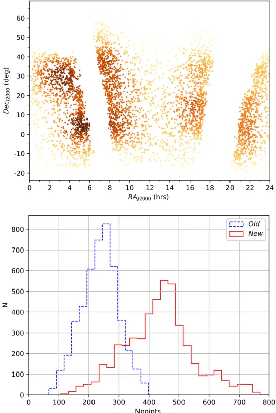
(2) The Astrophysical Journal Supplement Series, 238:4 (14pp), 2018 September. the time span of the LC), returning the top 5 peaks of the spectrum. The phase-folded LCs were visual inspected using these periods, and the best values were adopted. When the period values from AoV failed to phase-fold the LCs adequately, the other methods were applied, and the phased LCs were again visually inspected. A common issue encountered using periodograms, in the case of EBs, is the double/half period detection. For this reason, the majority of the phasefolded LCs were also examined using twice/half the detected period. Using the methodology described, we improved the period determination of the detached EB sample. While most of the new periods are in excellent agreement with those provided in Drake et al. (2014b), improved values are now available for ∼10% of the 4680 stars (Figure 2). Table 1 summarizes the results obtained for the latter, also including also the mean photometric error (Verr)8 and source coordinates (R.A.J2000, decl.J2000).. 2. Observations Observations were carried out during 2004–2016 using the three telescopes of the CSSs of Drake et al. (2009),6 covering the sky declination range δ = [−75, +65] deg, but avoiding crowded stellar regions within 10°–15° of the Galactic plane. The main goal of the survey is to discover near-Earth objects and potential hazardous asteroids. Nevertheless, time-series photometry for ∼200 million variable sources has been accumulated through CSS. In order to maximize the throughput, the observations are taken unfiltered, and the magnitudes are transformed to an approximate V magnitude (VCSS; Drake et al. 2013). The photometry was performed using the aperture photometry program SExtractor (Bertin & Arnouts 1996). In this study, we use Catalina Surveys Data Release 27 (CSDR2) with additional, not publicly accessible data, spanning 12 years (2004–2016). We focus on the sample of Drake et al. (2014b) of 4683 eclipsing binaries originally classified as EA type on the basis of 8 years of data. These cover a region of right ascension (R.A.) between 0 and 24 hr and declination (decl.) between −22° and +65°, as shown in Figure 1 (top). The bottom panel of Figure 1 shows the distribution of the new available data used in the present paper against the CSDR2 data. The total number of photometric points for the candidate systems that we studied significantly exceeds that available in the previous release.. 3.2. LC Phenomenological Parameters After phase-folding the LCs as explained in the previous subsection, long-term variations were also removed, when present (see Section 5). The LC was then fitted using the LMFIT9 (Newville et al. 2016) module in Python10 in order to derive its morphological features. Three different models were used, namely a chain of second-order polynomials (Prša et al. 2008; Papageorgiou et al. 2014), Fourier series fitting and a two-Gaussian model (TGM, Mowlavi et al. 2017). The actual fitting process was overseen by the Levenberg–Marquardt (LM, Levenberg 1944; Marquardt 1963) nonlinear minimization algorithm. We found that the TGM technique was much more robust and efficient, when applied to the stars in our sample. The procedure is based on modeling the geometry of LCs using Gaussian functions (to model the eclipses) and a cosine function (to model ellipsoidal variability, if present). Fitting a TGM to a time-series is very sensitive to the adopted initial values of the parameters. We therefore used the LM parameter values as starting points on each TGM. These included the phases (μi), the half widths (si), and the depths (di) of the primary and secondary eclipses (i = 1, 2), the peak-to-peak amplitude of the ellipsoidallike variation (Aell), and a constant (C) that equals the maximum light of the LC in the case of detached systems (Mowlavi et al. 2017, see their Figure 1). Since the success of modeling the folded LCs depends on the time sampling, measurement uncertainties, initial guessing of eclipse locations, and additional intrinsic variability in one or both stars of the binary system, a Markov Chain Monte Carlo (MCMC) analysis was performed on each TGM of our LC. 3. Identification of Algol-type Eclipsing Binaries in Catalina Sky Survey As we wanted to take all good data points of an LC into account to search for periodic signals, we first cleaned the 4683 LCs of the initial sample. For every LC a sigma-clipping cutoff algorithm was used to discard erroneous data points with values outside the interval of ±5σ of the median relative flux, where σ denotes the standard deviation computed from the whole LC. Furthermore, by adopting a pre-defined period from Drake et al. (2014b), we performed 5σ clipping from the median value of each phase bin. Therefore, we avoid rejecting data points corresponding to an eclipse and we ensure that the data points with errors larger than 5σ are discarded as outliers, presumably due to unreliable measurements. 3.1. Period Search After cleaning and checking a certain number of the resultant LCs, we applied a series of period-finding methods: 1. Analysis of Variance (AoV, Schwarzenberg-Czerny 1989, and Devor 2005); 2. Box-Least Squares (BLS, Kovács et al. 2002); 3. Generalized Lomb–Scargle (GLS, Press et al. 1992; Zechmeister & Kürster 2009); 4. Phase Dispersion Minimization (PDM, Stellingwerf 1978); and 5. Correntropy Kernelized Periodogram (CKP, Protopapas et al. 2015).. 8 The original CSS photometric errors are significantly overestimated, as discussed in Graham et al. (2017). Graham et al. provide a corrective factor fcorr to compensate for this problem. The following analytical fit provides an excellent description of the data shown in Figure1 of their paper: - + ⎡ (V - b)2 ⎤ ( 2 2 ) fcorr = a ⎢1 + , ⎥ ⎣ c 2d ⎦ d. The AoV, BLS, and GLS algorithms were applied through the command line utility VARTOOLS (Hartman & Bakos 2016). At first, the AoV method was applied, using a period range of [0.1–700] days and frequency resolution 0.1/T (where T is 6 7. Papageorgiou et al.. 1. (1). with a=1.350, b=19.491, c=3.006, and d=0.275. The fit is valid between V=14.0 and 19.5mag. For V<14.0 mag, a value fcorr=0.26 is assumed; for V>19.50 mag, we adopt instead fcorr=1.35. All error values reported in this paper, including tables and plots, have been corrected according to this recipe. 9 https://doi.org/10.5281/zenodo.11813 10 http://www.python.org. http://catalinadata.org http://nesssi.cacr.caltech.edu/DataRelease/. 2.

(3) The Astrophysical Journal Supplement Series, 238:4 (14pp), 2018 September. Papageorgiou et al.. Figure 1. Top: sky distribution of 4683 EBs in the CSS catalog. Bottom: distribution of the total number of photometric points per LC. The binary systems from the previous (Drake et al. 2014b) and new data releases (with the additional available data) are marked in the blue and red histograms, respectively.. sample, using the pyMC (Fonnesbeck et al. 2015) module11 in Python. The MCMC process begins by generating initial guesses for all the parameters randomly selected from a normal distribution based on the final LM fitting parameter values and errors. The new fit is accepted or rejected using the Metropolis– Hastings algorithm (Hastings 1970), compared to the fitting carried out in the previous step. In order to avoid the biases that 11. might be present in the initial solutions, the first 15,000 steps (of 200,000 steps in total) were discarded in the process. We then sampled this new synthetic model and discovered that the initial TGM model was noticeably different in some cases (Figure 3). Examples of the folded LCs, classified as D and SD as discussed below, are presented in Figure 4. The derived phenomenological parameters for 4680 EBs are presented in Table 2. Such parameters include: the magnitude at primary (MinI) and secondary eclipse (MinII), the magnitude at. https://pymc-devs.github.io/pymc/. 3.

(4) The Astrophysical Journal Supplement Series, 238:4 (14pp), 2018 September. Papageorgiou et al.. Figure 2. Refined periods of 4680 EB stars. While most of the new periods (Pernew) are in excellent agreement with those provided in Drake et al. (2014a, Perold), improved values are now available for ∼10% of the stars. The differences are mostly due to aliases. Table 1 CRTS EA Systems ID. R.A. (h:m:s). Decl. (° : ′ : ″). MJDa (days). Per (days). áVerrñb (mag). Npoints. Class. LMCand. LongTerm. 11291130655 11381030196 11291130352 10011280051 11291130739 11381030654 11291130763 11381030304 10011280091 11400990133 11041280214 11121260136 10011280269 10011280381 11121260465 11400990337 11381030834 11261160472 11351060279 11211200175 11181220236 10011270462 11400980842 11071260052 11261150467 11351050807 10011270364 11071260081 11400980526 11261150363 11381020853. 23:59:45.5 23:58:56.7 23:58:16.7 23:57:56.9 23:57:15.5 23:55:38.3 23:54:44.8 23:54:01.4 23:53:13.6 23:52:27.0 23:51:51.3 23:51:04.0 23:49:52.4 23:49:39.6 23:48:50.3 23:48:28.2 23:48:27.2 23:48:26.5 23:48:19.9 23:47:34.4 23:47:00.0 23:45:54.3 23:45:02.5 23:44:39.7 23:43:48.2 23:43:39.1 23:43:31.2 23:43:06.1 23:42:30.6 23:41:37.0 23:41:16.3. +30:37:31.8 +37:18:23.5 +29:33:25.3 −02:32:47.2 +30:54:55.4 +38:47:23.1 +30:57:51.9 +37:40:29.7 −02:18:50.2 +39:55:15.3 +03:54:09.0 +11:56:51.3 −01:20:59.4 −00:42:57.1 +13:33:00.1 +40:32:40.1 +39:20:32.8 +27:12:03.6 +34:48:33.9 +20:33:31.9 +18:00:15.6 −00:31:31.1 +41:54:19.9 +05:52:55.8 +27:06:30.4 +36:29:01.2 −01:03:54.4 +06:03:47.7 +41:01:39.8 +26:44:53.2 +39:22:34.6. 54265.53875 55062.35518 53537.41966 54747.25303 53563.82135 55508.59468 54394.71148 56558.31886 53655.26418 53694.94006 55850.15160 54095.14156 53637.21180 55113.21426 55858.22093 55119.12598 55348.41153 54732.19943 55943.75582 55088.41305 54480.10645 54477.07608 54632.41237 56301.08055 55024.49074 55366.42500 54009.17422 54730.34298 54394.14236 55009.56074 53655.20953. 2.68651 1.35464 0.72949 1.74457 2.84991 0.46792 0.82131 0.50473 0.50952 1.5311 2.98858 0.81240 1.76549 0.49138 1.46550 0.93421 1.70451 0.86780 2.52099 0.86457 3.07628 0.69255 0.85779 0.50740 2.15783 0.31764 1.13869 3.6267 0.52837 0.33624 0.70380. 0.0138 0.0136 0.0457 0.0133 0.0157 0.0356 0.0279 0.0232 0.0152 0.0287 0.0136 0.0138 0.0390 0.0345 0.0288 0.0182 0.0172 0.0237 0.0130 0.0144 0.0169 0.0234 0.0763 0.0136 0.0135 0.1027 0.0147 0.0335 0.0256 0.1115 0.0213. 391 312 390 325 381 312 349 312 325 218 375 442 325 324 442 219 308 371 326 429 431 398 245 407 438 386 398 407 248 436 325. D D SD N/A D N/A D D D D D D D D D N/A N/A D N/A D D D D SD D D D D D D D. L L L L L L L L L L L L L L L L L L L L L L L L L L L L L L L. L L L L L L L L L L L L L L L L L L L L L L L L L L L L L L L. Name CSS_J235945.5+303731 CSS_J235856.7+371823 CSS_J235816.7+293325 CSS_J235756.9–023247 CSS_J235715.5+305455 CSS_J235538.3+384723 CSS_J235444.8+305751 CSS_J235401.4+374029 CSS_J235313.6–021850 CSS_J235227.0+395515 CSS_J235151.3+035409 CSS_J235104.0+115651 CSS_J234952.4–012059 CSS_J234939.6–004257 CSS_J234850.3+133300 CSS_J234828.2+403240 CSS_J234827.2+392032 CSS_J234826.5+271203 CSS_J234819.9+344833 CSS_J234734.4+203331 CSS_J234700.0+180015 CSS_J234554.3–003131 CSS_J234502.5+415419 CSS_J234439.7+055255 CSS_J234348.2+270630 CSS_J234339.1+362901 CSS_J234331.2–010354 CSS_J234306.1+060347 CSS_J234230.6+410139 CSS_J234137.0+264453 CSS_J234116.3+392234. Notes. a Epoch at primary minimum. b Mean photometric error (VCSS). (This table is available in its entirety in machine-readable form.). maximum light out of the eclipses (MaxI), the difference between the eclipse depths (MinI–MinII), the amplitude (Amp), and the mean magnitude (áVmagñ). The histograms of the distribution of errors for the phenomenological parameters are shown in Figure 5.. (2015), using the Method for Eclipsing Component Identification (Devor & Charbonneau 2006), found 272 SD EBs among 2170 fitted LCs (of the total 4683), based on Roche lobe filling criteria. Based on the system morphology classification, we performed, for the first time, an automated classification of the majority of EA-type CSS EBs with machine-learning algorithms. In our search, unsupervised machine-learning followed, by supervised learning, was performed using 8000 synthetic LCs of D, SD,. 4. Classification The EBs in previous CSS data releases were classified into D or SD systems based on visual inspection of the LCs. Lee 4.

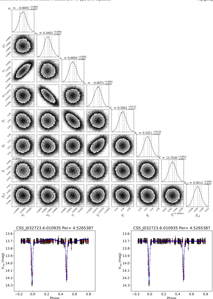
(5) The Astrophysical Journal Supplement Series, 238:4 (14pp), 2018 September. Papageorgiou et al.. Figure 3. Top: one-dimensional and two-dimensional projections of the posterior probability distributions (Foreman-Mackey et al. 2014) of a few parameters inferred from the TGM on each light curve. Bottom: example light curve with the initial (left) and the final (right) TGM fitting coupled by MCMC. The blue dots and solid lines refer to the resulting TGM, while the red dots refer to the CSS data. CSS IDs and periods are given at top of each light curve.. 5.

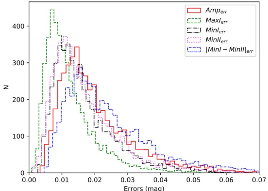
(6) The Astrophysical Journal Supplement Series, 238:4 (14pp), 2018 September. Papageorgiou et al.. Figure 4. Representative examples of a D system (left) and an SD system (right), obtained using TGM fitting. The symbols and colors are the same as those in Figure 3. CSS IDs and periods are given on top of each light curve. Table 2 Phenomenological Parameters of 4680 EBs Name. Amp (mag). Amperra (mag). MinI (mag). MinIerra (mag). MinII (mag). MinIIerra (mag). MaxI (mag). MaxIerra (mag). ∣MinI–MinII∣ (mag). ∣MinI–MinII∣err a (mag). CSS_J235945.5+303731 CSS_J235856.7+371823 CSS_J235816.7+293325 CSS_J235756.9–023247 CSS_J235715.5+305455 CSS_J235538.3+384723 CSS_J235444.8+305751 CSS_J235401.4+374029 CSS_J235313.6–021850 CSS_J235227.0+395515 CSS_J235151.3+035409 CSS_J235104.0+115651 CSS_J234952.4–012059 CSS_J234939.6–004257 CSS_J234850.3+133300 CSS_J234828.2+403240 CSS_J234827.2+392032 CSS_J234826.5+271203 CSS_J234819.9+344833 CSS_J234734.4+203331 CSS_J234700.0+180015 CSS_J234554.3–003131 CSS_J234502.5+415419 CSS_J234439.7+055255 CSS_J234348.2+270630 CSS_J234339.1+362901 CSS_J234331.2–010354 CSS_J234306.1+060347 CSS_J234230.6+410139 CSS_J234137.0+264453 CSS_J234116.3+392234. 1.9357 0.2647 1.4841 0.6316 0.3071 0.2798 0.8093 0.3562 0.7300 0.7084 1.0865 0.3206 1.0510 0.4143 0.5252 0.2586 0.3341 0.4481 1.3043 0.7597 0.3179 0.8222 0.6371 0.4433 0.5531 0.7290 0.1887 0.8140 0.3710 0.7832 0.6616. 0.0225 0.0083 0.0276 0.0344 0.0087 0.0150 0.0271 0.0283 0.0209 0.0145 0.0186 0.0128 0.0264 0.0217 0.0190 0.0110 0.0140 0.0109 0.0420 0.0145 0.0088 0.0161 0.0464 0.0165 0.0119 0.0426 0.0051 0.0196 0.0140 0.0390 0.0150. 15.6800 13.5267 18.2052 13.3882 14.6847 16.6196 16.7195 15.7998 15.0009 16.6152 14.3761 14.0039 17.5661 16.7682 16.4847 15.1143 14.9943 15.9527 12.7552 14.8161 14.9473 16.3255 18.1580 13.5755 13.7762 18.6783 14.3634 17.0581 16.0309 18.7695 15.8778. 0.0205 0.0061 0.0231 0.0269 0.0082 0.0117 0.0188 0.0205 0.0173 0.0112 0.0159 0.0105 0.0219 0.0166 0.0175 0.0091 0.0120 0.0088 0.0366 0.0123 0.0072 0.0132 0.0394 0.0130 0.0108 0.0311 0.0045 0.0188 0.0107 0.0323 0.0119. 13.8708 13.3597 16.9536 13.2883 14.6709 16.4139 16.5878 15.7252 14.8783 16.0845 13.3307 13.9033 16.7182 16.4422 16.2129 15.1082 14.7398 15.8867 11.8263 14.3558 14.9158 15.8831 18.0035 13.3442 13.7734 18.3661 14.2967 16.6652 15.7939 18.4569 15.3690. 0.0130 0.0069 0.0242 0.0288 0.0076 0.0152 0.0268 0.0240 0.0214 0.0100 0.0121 0.0130 0.0194 0.0153 0.0172 0.0153 0.0562 0.0097 0.0086 0.0187 0.0085 0.0151 0.0285 0.0142 0.0200 0.0364 0.0074 0.0158 0.0117 0.0328 0.0106. 13.7176 13.2358 16.6789 12.7309 14.3497 16.3397 15.8768 15.4119 14.2432 15.8725 13.2895 13.6566 16.4766 16.3179 15.9255 14.8268 14.6316 15.4728 11.4509 14.0290 14.6010 15.4719 17.4683 13.1060 13.1970 17.8895 14.1473 16.2079 15.6270 17.9221 15.1853. 0.0145 0.0062 0.0180 0.0239 0.0031 0.0104 0.0214 0.0217 0.0132 0.0103 0.0107 0.0079 0.0165 0.0161 0.0081 0.0069 0.0079 0.0072 0.0230 0.0083 0.0056 0.0103 0.0268 0.0112 0.0054 0.0323 0.0025 0.0060 0.0100 0.0261 0.0101. 1.8092 0.1669 1.2516 0.0999 0.0137 0.2057 0.1317 0.0745 0.1225 0.5306 1.0454 0.1006 0.8479 0.3259 0.2718 0.0061 0.2544 0.0659 0.9289 0.4602 0.0315 0.4424 0.1544 0.2313 0.0028 0.3121 0.0667 0.3928 0.2369 0.3125 0.5088. 0.0216 0.0088 0.0321 0.0379 0.0111 0.0192 0.0316 0.0301 0.0268 0.0143 0.0200 0.0164 0.0283 0.0211 0.0243 0.0175 0.0574 0.0128 0.0376 0.0222 0.0109 0.0195 0.0473 0.0187 0.0226 0.0458 0.0086 0.0244 0.0153 0.0438 0.0154. Note. a Estimated from the fitting. (This table is available in its entirety in machine-readable form.). overcontact (OC), and ellipsoidal (ELL) EBs. As a training set, 2000 LCs were randomly selected for each class, out of a total of ∼32,000 synthetic LCs. The synthetic LCs were created by a Monte Carlo-based script (Prša et al. 2008) in PHOEBE-scripter (Prša & Zwitter 2005), using randomly selected parameters for. each physical model. For each LC, 201 equally phased bins in the range [0, 1] were utilized. An unsupervised learning was then performed for each of 4050 phenomenological models obtained from Section 3.2, selected according to fitting performance. This was done by 6.

(7) The Astrophysical Journal Supplement Series, 238:4 (14pp), 2018 September. Papageorgiou et al.. Figure 5. Distribution of the obtained uncertainties in the parameters Amp, MaxI, MinI, MinII, and the difference ∣MinI–MinII∣.. Figure 6. Lower-dimensional input data space projection (2D projection) applying the method of Isomap. The axes of the 2D projection represent the top two eigenvectors of the geodesic distance matrix. The colored symbols indicate the distribution of synthetic LCs, whereas the black dots indicate the positions of CSS sources.. applying a variety of methods through the scikit-learn12 module (Pedregosa et al. 2012) in Python. Lower-dimensional space projections (2D and 3D) were found by applying the method of complete isometric feature mapping with 160 nearest neighbors (Isomap, Tenenbaum et al. 2000) that separated the classes (Figure 6). Considering the separation of the classes, we applied a supervised machine-learning using the values of the 3D projection as input for the training set and the CSS data. Furthermore, random Gaussian noise with a σ=0.08 mag was added to the sample of the training set and the phenomenological models. A variety of classifiers were applied, and we found that the best performance (validation score 92%) was achieved by Support Vector Machine (SVM). However, similar validation scores (∼89%–91%) were achieved using Random Forest, Artificial Neural Network (ANN), and K-nearest neighbor (KN) classifiers. 12. Table 3 Confusion Matrix of the SVM Classifier on 2000 Synthetic Test EBs. D SD OC ELL contam.. D. SD. OC. ELL. 525 3 0 1 0.01. 1 411 4 22 0.06. 0 8 470 4 0.02. 1 77 2 471 0.14. The confusion matrix of 2000 test synthetic EBs from the SVM classifier is presented in Table 3. We found a discrepancy among the classifiers for 263 EBs. Finally, after visual inspection, 54 systems were classified into D, 64 into SD, and 145 into D/SD. Therefore, the final catalog, presented in Table 1, contains 3456 D (85%), 449 SD (11%), and 145 EBs (4%) with uncertain classification (D/SD).. http://scikit-learn.org/stable/index.html. 7.

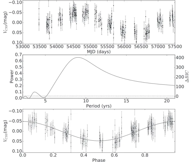
(8) The Astrophysical Journal Supplement Series, 238:4 (14pp), 2018 September. Papageorgiou et al.. Figure 7. Representative example of an EB (CSS J083938.7–050614) showing long-term variation in maximum light. Shown here is the result from applying a GLS periodogram to the residuals after subtracting the phenomenological model. Top: the residuals of the time-series data after subtraction of the TGM phenomenological model. Middle: GLS periodogram analysis of the residuals as a function of time. The dashed lines represent the 1σ and 3σ significance levels derived from 1000 Monte Carlo re-samplings. Bottom: residuals of the time-series data phased with the period derived from the periodogram.. timescales, the following set of constrains was applied to the results of the above methods:. 5. Long-term Variations Many phased LCs revealed scattering around maximum light, i.e., different maxima in brightness, as shown in Figures 7 and 8. This made us search for possible long-term changes over the 12-year time span of observations. To detect such variations, we applied three methods. In the first one (Method 1) we subtracted the TGM phenomenological model from the time-series observations (Figure 7, top) and performed a GLS analysis of the residuals (Figure 7, middle), in order to evaluate the possible presence of periodicity in this variation (Figure 7, bottom). For the second and third methods, prior to the fitting, the LCs were binned in time, with bin sizes that depended on the dynamical range of observations, and the median value and standard deviation were calculated for each such bin. Then, the eclipses were removed by selecting the data points in the neighborhood of the median values, applying 1σ tolerance (Figure 8, top right). The amplitude and the period of binned LCs were calculated through a GLS periodogram using the FATS library (Nun et al. 2015) in Python (Method 2) or by applying a harmonic fit to the binned data (Method 3). In order to detect significant variations over long (∼5–10 years). 1. LCs with amplitudes of the maxima variation lower than the LC mean error were rejected. 2. LCs with periods of maxima variation 800 days or 7000 days were rejected, due to the available time span of the observations. The upper limit is set by the fact that the total time baseline of the current sample of data of CSS survey is about 12years. Thus, the period of any parabolic variation must be less than roughly 1.5×12 years. 3. Only signals with a Bayesian Information Criterion (BIC, Schwarz 1978) greater than 15 were accepted. 4. Peak GLS power must be five times the 3σ power as predicted by 1000 Monte Carlo re-samplings (VanderPlas et al. 2012, 2014; Marsh et al. 2017). Combining the results from the previous methods and applying the aforementioned criteria, we found 152 systems in the sample of 4680 EBs that appear to exhibit variability in their maxima. For all these systems, the variability seems to be either periodic or quasi-periodic, over long (∼5–10 years) 8.

(9) The Astrophysical Journal Supplement Series, 238:4 (14pp), 2018 September. Papageorgiou et al.. Figure 8. Top: for the same star shown in Figure 7, we show here the light curves before (left) and after (right) removal of the long-term trend. Bottom: a harmonic fitting (solid line) was performed on the maximum light after the removal of the eclipses using the method described in Section 5.. timescales. Figure 8 (bottom) shows a representative example with the derived sinusoid model (Method 3) fitted on timebinned data. The resulting sample was examined for the possibility of the presence of SDSS (Ahn et al. 2012; Alam et al. 2015) sources within 5″ of our systems, as any such nearby sources could contaminate the CSS photometry and thus produce spurious variations in the LCs. As a result, 33 EBs were removed from the sample, resulting in 119 EBs with maximum light variation. This final sample of 119 EBs showing long-term variations in the maximum light is labeled in Table 1 as “LongTerm +.”. 5.1. Applegate Mechanism versus Spot Activity Maximum light variations in EBs can be explained by the Applegate mechanism (Applegate 1992) that relates the orbital period modulation to the operation of a hydromagnetic dynamo in the convection zone of the active star in a close binary system. As the active star progresses through its magnetic activity cycle, a changing differential rotation modifies its shape, changing the gravitational quadrupole moment that manifests itself through a cyclically varying orbital period and luminosity of the star, with the same period as the magnetic cycle. Fractional luminosity variations of ΔL/L∼0.1 of the 9.

(10) The Astrophysical Journal Supplement Series, 238:4 (14pp), 2018 September. Papageorgiou et al.. Figure 9. Time-series (left) and phase-folded data (right) of a simulated spotted EB with a magnetic cycle of 6.3years.. noise was added to the time-series data, and finally 300 random points were selected for the final simulated LC. The results of the simulation, under our assumptions (variable size of cool starspot regions), support the explanation of starspot activity (Figure 9). However, in order to achieve amplitudes of variation comparable to our observations and to cover regions that could produce variations also in out-of-eclipse phases, the starspot regions must be large; otherwise, we have to assume that both components show magnetic activity. Both the Applegate mechanism and starspot activity share the same period of the magnetic cycle of the magnetically active star. Accurate times of minimum light observations and period variation analysis are needed to investigate which mechanism(s) may be the underlying cause of these variations.. active(s) star(s) can produce period variations of ΔP/P∼10−5. The majority of our 119 candidates matching Two Micron All-Sky Survey (2MASS; Skrutskie et al. 2006) sources have colors J−H>0.237 mag and H−K>0.063 mag, which implies effective temperatures likely lower than ∼6200K (Pecaut & Mamajek 2013). Since our results are in agreement with the changes expected under the Applegate mechanism, the latter cannot be excluded as an explanation of the detected maximum light variations. However, if the convective zone cannot respond fast enough (i.e., the thermal timescale of the envelope is much longer than the timescale of the activity cycles), the heat flow variations will be dumped, and thus become unobservable (Watson & Marsh 2010; Khaliullin & Khaliullina 2012). On the other hand, maximum light variations could be explained by cool starspot coverage due to the magnetic activity. Our Sun shows such variations in a cycle of 11 years, and in case of low-mass EBs where the components are rotating nearly 100 times faster than the Sun, the deep convective envelope, along with rapid rotation, can produce a strong magnetic dynamo and solar-like magnetic activity. Long LCs shed light on the nature of the stellar activity of solar or late-type stars, either as single or as members of binary systems (such as BY Dra and RS CVn stars; Lehtinen et al. 2016). Marsh et al. (2017) suggested that the variation of the overall brightness in WUMa-type stars is probably caused by groups of starspots, rather than individual starspots. In order to simulate the effect of maximum light variations due to starspots, a synthetic eclipsing binary was constructed using the PHOEBE-2.0 engine (Prša et al. 2016) with two main-sequence stars with effective temperatures 5880 and 5490K. The inclination of the system was set to 80°. We assumed four starspot regions in order to simulate a uniform starspot coverage. The positions (longitude and colatitude) of the starspot regions were randomly drawn from a uniform distribution, and the temperature ratio of the spot over the star was set to 0.9 for the primary (active) star. In order to simulate the magnetic cycle, we assumed cyclic variations of the starspot radius (large enough to mimic starspot regions close to maximum activity, and small for lower magnetic activity) in the range of [0, 35] deg. A period of 6.3years was assumed for the magnetic cycle. For the virtual observations, a cadence of 300days and a total time-span of 9000days were assumed (i.e., we assumed that the virtual observations were carried out in one night every 300 days). Furthermore, variable random. 6. Low-mass Eclipsing Binaries in the Catalina Sky Survey Low-mass EB systems are interesting for determining the fundamental parameters of low-mass stars, which are the most common type of star in the universe. However, recent studies have shown that they represent significant challenges to the theoretical stellar models, due to their inflated sizes, magnetic activity, and also the poorly understood way they evolve in close binary systems (Chabrier et al. 2007; Feiden 2015; Zhou et al. 2015). Our list of 4050 classified EBs enables us to search for low-mass EB candidates by imposing color criteria. Accordingly, here we apply the following cuts: V−Ks>3.0, as suggested by Hartman et al. (2011) 0.35<J−H<0.8 mag, and H−Ks0.45 mag, based on Lépine & Gaidos (2011) and Zhong et al. (2015). For the color selection, we again use the 2MASS JHKs photometry, performing a cross-match to the 2MASS catalog (Cutri et al. 2003) within 3″ of the positions of our stars. Where available, photometry from the APASS survey (Henden et al. 2016) was also used, to obtain the (B − V ) color index in order to transform the VCSS magnitudes to Jonhson V. This was accomplished using the same transformation formula as presented in Drake et al. (2013): V = VCSS + 0.31 ´ (B - V )2 + 0.04. (2 ) This selects 2377 EBs. For the rest of the cataloged EBs for which we have no visual color information, we apply the transformation from 2MASS indices to the Johnson-Cousins system provided by Bilir et al. (2008, their Equation (16)). Interstellar extinction corrections were applied to the (B − V ) color index of each EB using the E(B − V ) values from Green et al. (2015). The VJHKs magnitudes were also corrected. 10.

(11) The Astrophysical Journal Supplement Series, 238:4 (14pp), 2018 September. accordingly, using extinction models obtained from a combination of Marshall et al. (2006), Green et al. (2015), and Drimmel et al. (2003), as included in the Python package mwdust13 (Bovy et al. 2016). Combining the results with the classification from Section 4, only the systems classified as D were finally accepted, resulting in 609 candidates. For distances between 1 and 4.5 kpc, the results are independent of the reddening corrections applied. To verify whether these are all bona fide low-mass EB candidates, we performed two tests:. determinations, phenomenological parameters of their LCs, and system morphology classifications based on machine-learning techniques. Our study includes many low-mass EB candidates, as well as systems that show additional variation in their maxima over long (∼5–10 years) timescales. Most of the new periods are in excellent agreement with those provided in the original Catalina catalogs, but significantly revised values have been obtained for ∼10% of the stars. A total of 3456 EBs were classified as D, 449 as SD, and 145 EBs had an uncertain classification. Our classification agrees with the findings of Lee (2015) for 83% of the sources. The sample classified as SD contains ∼9% systems with spectral types earlier than F0V, thus it seems that the majority of the systems in the sample are F-G spectral type EA systems with periods of less than a day. These systems have been characterized as short-period Algols (W CrV, Rucinski & Lu 2000) in the scenario of Stepien (2006). At the same time, they have also been described as being in near (CN And, Van Hamme et al. 2001; AX Dra, Kim et al. 2004) or broken (CN And, Van Hamme et al. 2001; Avvakumova et al. 2013) contact. We again caution, as we did in the introduction, that a detailed physical modeling of individual EBs is needed to reveal the true system configuration. Following our methodology of searching for K- and M-type dwarfs, we ended up with a sample of 609 low-mass EB candidates, increasing the total sample of stars at the low-mass end. Spectroscopic follow-up of these sources would be useful to help place constraints on models of low-mass stars. The majority of Lee’s (2015) low-mass candidates are included in our sample, including four that have been verified as doublelined M dwarf EBs (Lee & Lin 2017; Lee 2017). Moreover, we identified rare EA systems with periods close to the period cutoff at P∼0.22 day (Rucinski 1992, 1997). In addition to these results, our analysis of the long-term trends in the CSS data revealed cyclic or quasi-cyclic modulation of the maximum brightness on long (∼5–10 years) timescales for as many as 119 EA systems (2.5% of the entire sample). The ΔL/L range is within [0.04–0.13], with a mean value áDL Lñ = 0.075  0.017, while the periods are in the range of [4.5–18] years, with a mean P=12.1±3.3 years. Recently, Marsh et al. (2017) reported similar behavior in 205 eclipsing WUMa-type systems from CSS (2.2% of the target sample), finding periods in the range 4–11 years and fractional luminosity variance ΔL/L≈0.04–0.16. Close binaries are known to be significantly more active than wide binaries and single stars (e.g., Shkolnik et al. 2010), most likely due to their being tidally locked and high rotational velocities, resulting in high levels of magnetic activity. In late types this is predicted to inflate their radii by inhibiting convective flow and increasing starspot coverage. The observed long-term variability can be explained by either the Applegate mechanism or by variable spot regions. Oláh (2006) suggested that the magnetic field interaction has more effects on the starspot activities of the main-sequence stars than does the tidal force, because these stars have much higher surface gravities. As a consequence, the main-sequence stars often show active regions at quadrature phases. It should be noted that even though the vast majority of spotted stars cannot be easily imaged with special techniques (Doppler imaging or interferometry), our sample is useful to the future study of stellar activity cycles or other associated phenomena (e.g., flares).. 1. We compare their infrared colors with the theoretically expected colors of main-sequence F5-M3 dwarfs, as reported by Pecaut & Mamajek (2013). The results are shown in the upper panel of Figure 11. The reddening vector in this plot was calculated from the mean value of the extinction of the entire sample; 2. We compare their infrared colors with the colors of stars in the largest K and M dwarf spectroscopic sample (2612 binaries) from the Large Sky Area Multi-object Fiber Spectroscopic Telescope (LAMOST, Zhong et al. 2015). The results are shown in the lower panel of Figure 11. The periods of the final sample are in the range of [0.2–3.5] days (Figure 12). As we can see, the large majority of our sample does indeed fall within the K5 and M3 subtypes. These 609 binaries selected as low-mass candidates are marked in Table 1 as “LMcand +.” Examination of Table 1 in Lee (2015) reveals a total of 572 EB systems with nominal component masses <0.6 Me. However, as explained in that table’s header, this includes a large number of systems with uncertain solutions, and also systems with large errors (>0.2 Me) in the mass values. For this reason, to carry out a meaningful comparison between our results and those reported by Lee (2015), we restrict ourselves to systems with masses in the range covered by our sample (i.e., with spectral types later than K5, or masses <0.71 Me) and with errors <0.1 Me. This leads to a total of 107 systems, including 7 EBs classified as either nondetached or uncertain by our analysis, but which Lee classifies as detached. Out of the remaining 100, 72 were matched with our low-mass sample. The remaining 28 systems fall outside the limits of our color selection criteria, thus suggesting that they may not be bona-fide low-mass EB systems. Note that four systems have been verified as double-lined M-dwarf EBs (Lee & Lin 2017; Lee 2017); all of them are included in our sample of 609 candidates, but only two appear in Lee’s (2015) catalog. In addition, in our low-mass sample of detached EBs we found candidates near the short-period cutoff at P∼0.22 day (Rucinski 1992, 1997), as can be seen from Figure 10. Only a few such systems are currently known (Drake et al. 2014a). To our knowledge, the detached system with main-sequence components with the shortest period known (0.1926 day) is GSC 2314-0530 (=1SWASP J022050.85+332047.6), identified by Norton et al. (2007) and modeled by Dimitrov & Kjurkchieva (2010). Nefs et al. (2012) spectroscopically confirmed a detached system with a 0.18day period containing an M dwarf, but without measuring radial velocities. 7. Conclusions Using CSS data covering a 12-year time span, we obtained an updated catalog of 4680 EA-type EBs, with revised period 13. Papageorgiou et al.. https://github.com/jobovy/mwdust. 11.

(12) The Astrophysical Journal Supplement Series, 238:4 (14pp), 2018 September. Papageorgiou et al.. Figure 10. Folded LC of CSS J041918.8–071807, the low-mass EB candidate with the shortest period (P=0.22 days) in our sample.. A.P. and M.C. gratefully acknowledge the support provided by Fondecyt through grants #3160782 and #1171273. Additional support for this project is provided by the Ministry for the Economy, Development, and Tourism’s Millennium Science Initiative through grant IC 120009, awarded to the Millennium Institute of Astrophysics (MAS); by Proyecto Basal PFB-06/2007; and by CONICYT’s PCI program through grant DPI20140066. M.C. gratefully acknowledges the additional support provided by the Carnegie Observatories through its Distinguished Scientific Visitor program. The Monte Carlo script in PHOEBE-scripter is based on the script that was kindly provided by Dr. Andrej Prša. This work made use of data products from the CSS survey. The CSS survey is funded by the National Aeronautics and Space Administration under grant No. NNG05GF22G issued through the Science Mission Directorate Near-Earth Objects Observations Program. The CRTS survey is supported by the US National Science Foundation under grants AST-0909182, AST-1313422, AST-1413600, and AST-1518308. This publication makes use of data products from the Two Micron All Sky Survey, which is a joint project of the University of Massachusetts and the Infrared Processing and Analysis Center/California Institute of Technology, funded by the National Aeronautics and Space Administration and the National Science Foundation. Funding for SDSS-III has been provided by the Alfred P. Sloan Foundation, the Participating Institutions, the National Science Foundation, and the U.S. Department of Energy Office of Science. The SDSS-III website ishttp://www.sdss3.org/. This publication makes use of data products from SDSS-III. SDSS-III is managed by the Astrophysical Research Consortium for the Participating Institutions of the SDSS-III Collaboration including the University of Arizona, the Brazilian Participation Group, Brookhaven National Laboratory, Carnegie Mellon University, University of Florida, the French Participation Group, the German Participation Group, Harvard University, the Instituto de Astrofisica de Canarias, the Michigan State/Notre Dame/JINA Participation Group, Johns Hopkins University, Lawrence Berkeley National Laboratory, Max Planck Institute for Astrophysics, Max Planck Institute for Extraterrestrial Physics, New Mexico State University, New York University, Ohio State University, Pennsylvania State University, University of Portsmouth, Princeton University, the. Figure 11. Top: (V - Ks ) - (J - H ) color–color diagram of the 3456 CSS EBs classified as D and the theoretically expected colors of main-sequence F5M3 stars (Pecaut & Mamajek 2013). The large dots refer to the low-mass EB candidates. The reddening vector was calculated from the mean value of the extinction of the entire sample, while the range is within [0.01–0.59]mag. Bottom: (H - Ks ) - (J - H ) color–color diagram of 609 low-mass EB candidates (large dots) overplotted on the sample of low-mass stars from the LAMOST survey (smaller dots). In both panels, the different colors indicate the color index value according to the adjacent color bar.. Spanish Participation Group, University of Tokyo, University of Utah, Vanderbilt University, University of Virginia, University of Washington, and Yale University. This work has made use of the SIMBAD database, operated at CDS, Strasbourg, France. This research was made possible through the use of the AAVSO Photometric All-Sky Survey (APASS), funded by the Robert Martin Ayers Sciences Fund. Software: AstroML (VanderPlas et al. 2012), CKP (Protopapas et al. 2015), FATS (Nun et al. 2015), LMFIT (Newville et al. 2016), mwdust (Bovy et al. 2016), PDM (Stellingwerf 1978), PHOEBE-scripter (Prša & Zwitter 2005), PHOEBE-2.0 (Prša et al. 2016), pyMC (Fonnesbeck et al. 2015), scikit-learn (Pedregosa et al. 2012), triangle.py-v0.1.1 (Foreman-Mackey et al. 2014), VARTOOLS (Hartman & Bakos 2016). 12.

(13) The Astrophysical Journal Supplement Series, 238:4 (14pp), 2018 September. Papageorgiou et al.. Figure 12. Period distribution of 609 low-mass EB candidates identified in this study.. Appendix Acronyms and Abbreviations. Bertin, E., & Arnouts, S. 1996, A&AS, 117, 393 Bilir, S., Ak, S., Karaali, S., et al. 2008, MNRAS, 384, 1178 Bovy, J., Rix, H.-W., Green, G. M., Schlafly, E. F., & Finkbeiner, D. P. 2016, ApJ, 818, 130 Catelan, M., Dékány, I., Hempel, M., & Minniti, D. 2013, BAAA, 56, 153 Catelan, M., & Smith, H. A. 2015, Pulsating Stars (Weinheim: Wiley-VCH) Chabrier, G., Gallardo, J., & Baraffe, I. 2007, A&A, 472, L17 Christian, D. J., Pollacco, D. L., Skillen, I., et al. 2006, AN, 327, 800 Cutri, R. M., Skrutskie, M. F., van Dyk, S., et al. 2003, yCat, 2246 Devor, J. 2005, ApJ, 628, 411 Devor, J., & Charbonneau, D. 2006, ApJ, 653, 647 Dimitrov, D. P., & Kjurkchieva, D. P. 2010, MNRAS, 406, 2559 Drake, A. J., Catelan, M., Djorgovski, S. G., et al. 2013, ApJ, 763, 32 Drake, A. J., Djorgovski, S. G., Catelan, M., et al. 2017, MNRAS, 469, 3688 Drake, A. J., Djorgovski, S. G., García-Álvarez, D., et al. 2014a, ApJ, 790, 157 Drake, A. J., Djorgovski, S. G., Mahabal, A., et al. 2009, ApJ, 696, 870 Drake, A. J., Graham, M. J., Djorgovski, S. G., et al. 2014b, ApJS, 213, 9 Drimmel, R., Cabrera-Lavers, A., & López-Corredoira, M. 2003, A&A, 409, 205 Feiden, G. A. 2015, in ASP Conf Ser. 496, Living Together: Planets, Host Stars and Binaries, ed. S. M. Rucinski, G. Torres, & M. Zejda (San Francisco, CA: ASP), 137 Fonnesbeck, C., Patil, A., Huard, D., & Salvatier, J. 2015, PyMC: Bayesian Stochastic Modelling in Python, Astrophysics Source Code Library, ascl:1506.005 Foreman-Mackey, D., Price-Whelan, A., Ryan, G., et al. 2014, Zenodo Software Release, 2014 Graham, M. J., Djorgovski, S. G., Drake, A. J., et al. 2017, MNRAS, 470, 4112 Green, G. M., Schlafly, E. F., Finkbeiner, D. P., et al. 2015, ApJ, 810, 25 Hartman, J. D., & Bakos, G. Á 2016, A&C, 17, 1 Hartman, J. D., Bakos, G. Á, Noyes, R. W., et al. 2011, AJ, 141, 166 Hastings, W. K. 1970, Biometrika, 57, 97 Henden, A. A., Levine, S., Terrell, D., et al. 2015, American Astronomical Society Meeting Abstracts #225, 336.16. Khaliullin, K. F., & Khaliullina, A. I. 2012, MNRAS, 419, 3393 Kim, H.-I., Lee, J. W., Kim, C.-H., et al. 2004, PASP, 116, 931 Kovacs, G. 2017, EPJWC, 152, 01005 Kovács, G., Zucker, S., & Mazeh, T. 2002, A&A, 391, 369 Larson, S., Beshore, E., Hill, R., et al. 2003, BAAS, 35, 36.04 Layden, A. C. 1998, AJ, 115, 193 Lee, C.-H. 2015, MNRAS, 454, 2946 Lee, C.-H. 2017, AJ, 153, 118 Lee, C.-H., & Lin, C.-C. 2017, RAA, 17, 15 Lehtinen, J., Jetsu, L., Hackman, T., Kajatkari, P., & Henry, G. W. 2016, A&A, 588, A38 Lépine, S., & Gaidos, E. 2011, AJ, 142, 138 Levenberg, K. 1944, QApMa, 2, 164 Marquardt, D. W. 1963, SJAM, 11, 431 Marsh, F. M., Prince, T. A., Mahabal, A. A., et al. 2017, MNRAS, 465, 4678 Marshall, D. J., Robin, A. C., Reylé, C., Schultheis, M., & Picaud, S. 2006, A&A, 453, 635 Minniti, D., Lucas, P. W., Emerson, J. P., et al. 2010, NewA, 15, 433 Mowlavi, N., Lecoeur-Taïbi, I., Holl, B., et al. 2017, A&A, 606, A92 Nefs, S. V., Birkby, J. L., Snellen, I. A. G., et al. 2012, MNRAS, 425, 950. Description CSS VISTA ASAS NSVS VVV TrES OGLE HATNet SuperWASP 2MASS APASS LAMOST CSDR2 AoV BLS GLS PDM CKP MCMC SVM ANN KN BIC LM. Catalina Sky Survey Visible and Infrared Survey Telescope for Astronomy All Sky Automated Survey Northern Sky Variability Survey Variables in the Via Lactea Transatlantic Exoplanet Survey TrES Optical Gravitational Lensing Experiment Hungarian-made Automated Telescope Network exoplanet survey Wide Angle Search for Planets Two Micron All-Sky Survey AAVSO Photometric All-Sky Survey Large Sky Area Multi-object Fiber Spectroscopic Telescope Catalina Surveys Data Release 2 Analysis of Variance Box-Least Squares Generalized Lomb–Scargle Phase Dispersion Minimization Correntropy Kernelized Periodogram Markov Chain Monte Carlo Support Vector Machine Artificial Neural Network K-nearest neighbor Bayesian Information Criterion Levenberg–Marquardt nonlinear minimization algorithm. ORCID iDs Athanasios Papageorgiou https://orcid.org/0000-00023039-9257 Márcio Catelan https://orcid.org/0000-0001-6003-8877 S. G. Djorgovski https://orcid.org/0000-0002-0603-3087 References Ahn, C. P., Alexandroff, R., Allende Prieto, C., et al. 2012, ApJS, 203, 21 Alam, S., Albareti, F. D., Allende Prieto, C., et al. 2015, ApJS, 219, 12 Alonso, R., Brown, T. M., Charbonneau, D., et al. 2007, in ASP Conf. Ser. 366, Transiting Extrapolar Planets Workshop, ed. C. Afonso, D. Weldrake, & T. Henning (San Francisco, CA: ASP), 13 Alonso, R., Brown, T. M., Torres, G., et al. 2004, ApJL, 613, L153 Applegate, J. H. 1992, ApJ, 385, 621 Avvakumova, E. A., Malkov, O. Y., & Kniazev, A. Y. 2013, AN, 334, 860 Bakos, G., Noyes, R. W., Kovács, G., et al. 2004, PASP, 116, 266. 13.

(14) The Astrophysical Journal Supplement Series, 238:4 (14pp), 2018 September Newville, M., Stensitzki, T., Allen, D. B., et al. 2016, Lmfit: Non-Linear LeastSquare Minimization and Curve-Fitting for Python, Astrophysics Source Code Library, ascl:1606.014 Norton, A. J., Wheatley, P. J., West, R. G., et al. 2007, A&A, 467, 785 Nun, I., Protopapas, P., Sim, B., et al. 2015, arXiv:1506.00010 Oláh, K. 2006, Ap&SS, 304, 145 Palaversa, L., Ivezić, Ž, Eyer, L., et al. 2013, AJ, 146, 101 Papageorgiou, A., Kleftogiannis, G., & Christopoulou, P.-E. 2014, CoSka, 43, 470 Pecaut, M. J., & Mamajek, E. E. 2013, ApJS, 208, 9 Pedregosa, F., Varoquaux, G., Gramfort, A., et al. 2012, arXiv:1201.0490 Pojmanski, G. 1997, AcA, 47, 467 Pojmanski, G., Pilecki, B., & Szczygiel, D. 2005, AcA, 55, 275 Pollacco, D., Skillen, I., Collier Cameron, A., et al. 2006, Ap&SS, 304, 253 Press, W. H., Teukolsky, S. A., Vetterling, W. T., & Flannery, B. P. 1992(2nd ed.; Cambridge: Cambridge Univ. Press) Protopapas, P., Huijse, P., Estévez, P. A., et al. 2015, ApJS, 216, 25 Prša, A., Conroy, K. E., Horvat, M., et al. 2016, ApJS, 227, 29 Prša, A., Guinan, E. F., Devinney, E. J., et al. 2008, ApJ, 687, 542 Prša, A., & Zwitter, T. 2005, ApJ, 628, 426 Rucinski, S. M. 1992, AJ, 103, 960 Rucinski, S. M. 1997, MNRAS, 382, 393 Rucinski, S. M., & Lu, W. 2000, MNRAS, 315, 587 Schwarz, G. 1978, AnSta, 6, 461. Papageorgiou et al. Schwarzenberg-Czerny, A. 1989, MNRAS, 241, 153 Shkolnik, E. L., Hebb, L., Liu, M. C., Reid, I. N., & Collier Cameron, A. 2010, ApJ, 716, 1522 Skrutskie, M. F., Cutri, R. M., Stiening, R., et al. 2006, AJ, 131, 1163 Soszyński, I. 2017, EPJWC, 152 Stellingwerf, R. F. 1978, ApJ, 224, 953 Stepien, K. 2006, AcA, 56, 199 Stokes, G. H., Evans, J. B., Viggh, H. E. M., Shelly, F. C., & Pearce, E. C. 2000, Icar, 148, 21 Tenenbaum, J. B., de Silva, V., & Langford, J. C. 2000, Sci, 290, 2319 Torres, G., Andersen, J., & Giménez, A. 2010, A&ARv, 18, 67 Udalski, A., Szymanski, M., Kaluzny, J., Kubiak, M., & Mateo, M. 1992, AcA, 42, 253 Van Hamme, W., Samec, R. G., Gothard, N. W., et al. 2001, AJ, 122, 3436 VanderPlas, J., Connolly, A. J., Ivezic, Z., & Gray, A. 2012, arXiv:1411.5039 VanderPlas, J., Fouesneau, M., & Taylor, J. 2014, AstroML: Machine learning and data mining in astronomy Astrophysics, Source Code Library, ascl:1407.018 Watson, C. A., & Marsh, T. R. 2010, MNRAS, 405, 2037 Welsh, W. F., Orosz, J. A., Aerts, C., et al. 2011, ApJS, 197, 4 Woźniak, P. R., Vestrand, W. T., Akerlof, C. W., et al. 2004, AJ, 127, 2436 Zechmeister, M., & Kürster, M. 2009, A&A, 496, 577 Zhong, J., Lépine, S., Hou, J., et al. 2015, AJ, 150, 42 Zhou, G., Bayliss, D., Hartman, J. D., et al. 2015, MNRAS, 451, 2263. 14.

(15)