Accessing very high dimensional spaces in parallel

Texto completo

(1)Journal of Supercomputing manuscript No. (will be inserted by the editor). Accessing very high dimensional spaces in parallel F.J. Artigas-Fuentes · J.M. Badı́a. Received: date / Accepted: date. Abstract Access methods are a fundamental tool on Information Retrieval. However, most of these methods suffer the problem known as the curse of dimensionality when they are applied to objects with very high dimensionality representation spaces, such as text documents. In this paper we introduce a new parallel access method that uses several graphs as distributed index structure and a kN N search algorithm. Two parallel versions of the search method are presented, one based on master-slave scheme and the other based on a pipeline. A thorough experimental analysis on different datasets shows that our method can process efficiently large flows of queries, compete with other parallel algorithms and obtain at the same time very high quality results. Keywords parallel access method · high dimensional spaces · multiple graphs index. 1 Introduction One of the basic problems on Information Retrieval (IR) is the search in multidimensional spaces by spatial approximation [5]. A search space is formed by a collection of objects U and a similarity function s to compare them. The difference between metric and non-metric spaces is that on the first case s satisfies the triangle inequality, and becomes a distance d. The goal of an access method is to retrieve the most similar object or objects to a query q. Special methods must be designed when representation space has very large dimensionality, i.e. thousands of dimensions. In this case exact methods F.J. Artigas-Fuentes Facultad de Matemática y Computación, Univ. de Oriente. Santiago de Cuba, Cuba. Tel.: +53-22662189, E-mail: [email protected] J.M.Badı́a-Contelles Dept. de Ingenierı́a y Ciencia de los Computadores, Univ Jaume I, Castellón, España. Tel.: +34-964728295, Fax: +34-964728486, E-mail: [email protected].

(2) 2. F.J. Artigas-Fuentes, J.M. Badı́a. cannot be used due to the curse of dimensionality [22], which causes them to need an enormous quantity of space and time to reach the solutions. This happens because the strategies applied by those methods to reduce the portion of repository visited during the searches fail. For example, for access methods using a space partitioning strategy, a very high dimensionality causes a high degree of overlapping of candidate regions to find solutions to queries. Access methods applying a data partitioning strategy [1] also fail because they are unable to separate the data. In [2] we introduced an approximate access method, nGraph, composed by an index structure based on a single graph and a fast search algorithm based on the k − N N strategy. The method was designed to support efficient searches in very high dimensional spaces such as text document repositories. It was also used in a fast text documents classifier, with high quality results similar, or even better, than other state-of-art methods [3]. In IR we usually deal with a large flow of queries on very large datasets. The best way to tackle the spatial and computational cost of this problem is to implement parallel or distributed algorithms that can take advantage of the current high performance architectures [5]. In this paper we introduce P M Graphs, a parallel access method implemented with MPI. It includes both a distributed index structure based on multiple graphs, and a parallel search algorithm. We compare two parallel versions of the search process that exploit a master-slave and a pipeline scheme respectively. To evaluate our our algorithms, we carried out thorough experiments using images and text documents datasets on distributed and shared memory multiprocessors. We analyzed both the quality of the results and the efficiency of the method. The experiments show that our proposal greatly reduces the sequential cost of the index generation and search process, while preserving the quality of results achieved with nGraph. The rest of the paper is organized as follows: section 2 summarizes related work, section 3 describes the sequential version of our method, section 4 introduces our parallel proposal, section 5 includes our experiments and analysis of the results. Finally, in section 7 the conclusions of this paper are presented.. 2 Related work There is a huge quantity of literature about sequential similarity search methods, mostly on metric spaces [15]. Similarity search methods can be mainly classified as pivot or compact partitioning techniques. Other methods not clearly fitting into this two classes include for example some methods based on graph structures, such as kNN graphs [21]. State-of-the-art methods also include dimension reduction methods based on hashing techniques [13]. On the one hand, compact partitioning techniques divide the data collection into spatial zones as compact as possible so that similar objects fall into the same zone. Indexes store information about the partitions and are com-.

(3) Accessing very high dimensional spaces in parallel. 3. bined with the triangle inequality to solve the queries reducing the number of distance calculations. On the other hand, pivot techniques select some objects from the collection as pivots and then compute the distance between the pivots and the objects of the repository. For each query, a candidate list is built with the objects that cannot be discarded when compared with the pivots so they have to be compared directly with the query object. For example, permutation methods [19] are a kind of pivot method with dimension reduction. In [19] we can find a very good comparative analysis of several state-of-theart methods for approximate k-NN search. Experiments are performed with a large number of varied datasets represented in both metric and non-metric spaces. One of the main conclusions of the authors is that if we want high quality results, the method based on a k-NN graph outperforms the others in most cases. The main drawback of this method is a long indexing time. Regarding parallel methods, the most extended criterion to classify query processing depends on index partitioning among the processors. If we distribute the objects among the processors and each processor builds its own index, we are dealing with local index methods. If, on the other hand, we build an index including all the objects and then distribute it among the processors, we are dealing with global index methods. Another classifying criterion differentiates inter-query parallelism if different queries are executed concurrently and intra-query parallelism if different parts of the same query are executed in parallel. In a very recent paper [4] the author surveys the notable advancements in the parallelization efforts on nearest searching algorithms produced during the last years. One of the main conclusions of the author of this survey is that an optimal algorithm as well as removing the curse of dimensionality are still open problems. Different data structures have been proposed to index the objects in parallel, such as SAT [17], EGNAT [18] or SSS [10]. Many of the parallel nearest neighbor search proposals of the last years have been developed on single GPU or multi-GPU platforms [12]. Most of them use a brute force approach to solve the problem [14] and differ on the sorting strategies to get the kNN. However, there are also methods on GPU that parallelize the construction and use of different data structures as indexes [6] or use hashing techniques to reduce the dimensionality [20]. Many more references to parallel methods on GPU can be found in [4] and on the cited papers. We will compare our parallel algorithms with a parallel implementation of a compact partitioning method that uses a List of clusters (LC) [8] as index. This method builds the index by choosing a set of objects as centers c of clusters with radius rc . We have chosen a version of the algorithm where clusters contain a bucket that keeps the same number of closest elements to c. Buckets are filled sequentially as the centers are created. Queries are solved by scanning the centers in order of creation. Full clusters can be discarded during query processing based on the triangle inequality. There are several parallel algorithms that use the LC index on different kinds of parallel platforms: distributed memory [11] and shared memory [9].

(4) 4. F.J. Artigas-Fuentes, J.M. Badı́a. multiprocessors, GPUs [6] and multi-GPU platforms [7]. We will compare our parallel algorithms with the local version of the algorithm introduced in [9] to deal with high query traffic. This algorithm is implemented with OpenMP and uses inter-query parallelism to distribute the processing of different queries on different cores of a shared memory multiprocessor. A global LC index is built in parallel using several threads and it is accessed by the different threads that process different blocks of queries.. 3 Sequential access method M Graphs In this section we briefly describe the two main stages of our new sequential access method, M Graphs, that is, the construction of the index structure and the search process. To build the index structure we start by dividing the objects repository into several subsets, where each object is represented as a vector of weighted terms. For each subset the method builds a graph that fulfills the following conditions: (a) every vertex corresponds to a different vector, and a vector represents the set of objects whose similarity to that vector is 1 (or dissimilarity or distance is 0) and (b) the neighborhood of every vertex contains at least its δ more similar vertices, plus additional vertices to ensure that the graph is connected. Algorithm 1 summarizes the process followed to build each graph of the index. First we define a similarity function s(vi , vj ) between a pair of vectors. Then we can define a similarity function between a vertex vi and an edge aj = (vj1 , vj2 ) as d(vi , aj ) = min{d(vi , vj1 ), d(vi , vj2 )}. To build each graph we sort the list of vectors by their similarity to the centroid of the subset in decreasing order. Then, the first edge of the graph is defined between the most similar pair of vertices (line 7 of Algorithm 1). From this point on, the structure is built by adding new vertices that form the smallest triangles to the vertices already on the graph. The process continues until all the objects of the subset are connected (lines 8 to 15). To reduce the cost of the process we applied an heuristic that divides the sorted list of vertices of each graph in equal-sized groups (lines 5 and 6). When we add a new vertex to the graph we only compare it with the other vertices of its group (line 7). Therefore, we are building the graph as a succession of layers including the vertices in each group. Finally, once all vertices have been included, the graph is completed by adding new edges to each vertex until the graph fulfills condition (b) (lines 17 to 23). The index structure is completed by determining a subset of entry points to each graph that can be used as starting points for the searches (line 24). The outer entry points are the vertices closer to the centroid than their neighborhood and the inner entry points are the vertices farther to the centroid than their neighborhood. The resulting index structure is a set of graphs that are sequentially searched for each query q by spatial approximation to obtain the k − N N ..

(5) Accessing very high dimensional spaces in parallel. 5. Algorithm 1 Process to build each of the graphs of the index 1: function BuildGraph(V, δ) 2: Input. V : Set of vectors to index, δ: minimum degree of the graph. 3: Output. G: Graph of the index. P (vi [j]). and j = 1.. |V | . centroid 4: c ← (c[1], ..., c[|V |]) where c[j] = |V | 5: Build a sorted list with the objects of V in decreasing order of similarity with c 6: Partition the sorted list in Nl equal size lists: Vi , i = 1..Nl 7: Select from V1 a pair (vh , vk ), where s(vh , vk ) is maximum for V1 8: A ← {a1 }, so that a1 = {(vh , vk )} . Initial set of edges of G 9: V1 ← V1 − {vh , vk } 10: for k ← 1, Nl do . Build connected graph 11: while Vk 6= ∅ do 12: Select vh ∈ Vk and at ∈ A, so that s(vh , at ) is maximum. 13: A ← A ∪ {(vh , at [1]), (vh , at [2])}; Vk ← Vk − {vh } 14: end while 15: end for 16: for all vi ∈ V do . Complete the set of edges to fulfill minimum degree 17: while s(vi ) < δ do . s(vi ) is the degree of vi 18: C ← {vk /vk ∈ / NG (vi )} . NG (vi ) is the neighborhood of vi 0 . Edges of a A containing vi 19: A ← {ai /ai = (vi , vj ) ∈ A} 0 20: Select vh ∈ C and at ∈ A , so that s(vh , at ) is maximum. 21: C ← C − {vh }; A ← A ∪ {(vh , at [1]), (vh , at [2])} 22: end while 23: end for 24: E ← {vi ∈ V /entrypoint(vi )} . Set of entry points of G 25: return G = (V, A, E) 26: end function. Algorithm 2 summarizes the search process on each graph. First we obtain the most similar entry point to the query q (lines 5 and 6). Then we visit the neighborhood of the entry point and select as new starting point the most similar vertex to q. This process continues until we cannot find a more similar vertex to q in the neighborhood of the current point (lines 7 to 12). We have then obtained an approximate 1 − N N to the query. If more solutions are needed we quickly obtain the next k − 1 from the neighborhood of the first one. They are not necessarily obtained from most to least similar neighbors to the query, but they are finally stored in a sorted list using this criterion (lines 13 to 19). To extend the search process to all graphs in the index we apply successively the same algorithm to each of them keeping always an updated list L with the kN N obtained from the previous graphs. Each element of the list contains the identifier of the object and its similarity to the query. This list, sorted in decreasing order of similarity to the query, is updated with the local solution of the current graph as follows: if the first nearest neighbor computed in the current graph is less similar to the query than the last contained in the sorted list L, we can stop the query on process on the current graph and start with the next one. Otherwise, we compute the next k − 1 nearest neighbors in the local graph and merge them with the k contained in sorted list L keeping always the k most similar to the query..

(6) 6. F.J. Artigas-Fuentes, J.M. Badı́a. Algorithm 2 Approximate k-NN search on each graph of the index 1: function kN N (G, q, k) 2: Input. G = (V, A, E): graph of the index, 3: q: query vector, k: number of neighbours. 4: Output. Sq : k most related vertices of V with q, using similarity function d. 5: Select er ∈ E so that s(q, er ) = max{s(q, ei )/ei ∈ E}. 6: dmax ← s(q, er ) and Sq ← er . Most related pivot 7: repeat 0 8: NG ← {vk ∈ NG (Sq )/s(q, vk ) = max(s(q, vi )/vi ∈ NG (Sq ))} 0 0 9: Sq ← {vk ∈ NG (Sq )/s(q, vk ) > dmax } . Depth-first strategy 0. 0. 10: if Sq 6= ∅ then dmax ← s(q, vk ); Sq ← Sq 11: end if 0 12: until Sq = ∅ 13: if k > 1 then 14: repeat 0 . Greedy strategy 15: Sq ← Sq ; Sq ← Sq ∪ NG (Sq ) 16: Let L be a sorted list vi ∈ Sq , by decreasing value of s(vi , q) 17: Let N Pq be the set of the first k elements of L 18: until |N Pq | ≥ k 19: end if 20: return Sq 21: end function. We have tested our methods using different similarity functions. Some of them do not satisfy the triangle inequality. We can then apply our method to both metric and non-metric spaces, but in the second case we cannot exploit this property to define a pruning rule. When we tried to exploit it on a text document repositories with a very high dimensionality it did not work, as it trimmed either all or none of the candidate vertices.. 4 Parallel access method P M Graphs In this section we describe the parallelization of the two main stages of M Graphs. The index construction is naturally parallelizable, as it is composed by multiple graphs. In this case we only have to distribute the objects of the dataset among the processors, so that each processor applies the sequential method described in previous section to build its local graph. This parallel process can be completed without any kind of communication or synchronization among the processors. A possible problem of this parallel scheme is that the cost of building each local graph can be quite different, thus producing an unbalanced computation. Besides, the objects included on each graph also affect the efficiency of the subsequent parallel search process. Regarding the parallelization of the k−N N search process we implemented two parallel versions, each applying a classical parallelization scheme: a masterslave algorithm and a pipeline scheme. In the case of the master-slave algorithm, the master process broadcasts every query or block of queries to all the processes. Then all processes, including the master, compute the k − N N to the query in their local graphs by.

(7) Accessing very high dimensional spaces in parallel. 7. applying the sequential search algorithm described in previous section. Next, the local solutions of the queries are combined to obtain the global k − N N objects to the query and store them in the master process. Every neighbor in a graph is stored with its similarity to the query and the k − N N of the graph are stored in decreasing order of similarity. Therefore, if we want to combine the kN N neighbors of several graphs we can easily merge the local solutions to obtain the global k nearest neighbors to the query. Local solutions are gathered on the master, that combines them to obtain the global solution. To reduce the cost of this process we have implemented a binary tree communication scheme that parallelizes the combination of the local solutions. On each of the O(logp) steps of the scheme pairs of processors combine their local solutions in parallel, so that after the last step the master process can obtain the global k − N N by combining only two groups of k objects. In the second version of the parallel search algorithm the processors are organized as a pipeline. The first process of the pipeline obtains the k − N N objects to the query on its local graph and sends them, and the query, to the next process. Each of the following processes in the pipeline searches in their local graph trying to improve the received neighbors. Then it sends the resulting k candidates and the query to the next process. As we can see, every process is applying a slightly modified version of Algorithm 2 to obtain the local kN N to the received query. It does not need to compute always k neighbors as it can stop if the first computed local neighbor is less similar to the query than the last in the received list of candidates. As we are dealing with a large flow of queries, this pipeline search method with p processes will be evaluating in parallel p queries most of the time.. 5 Experimental testbed We will show experimental results of our parallel algorithms using two different datasets. Images contains 120,000 vectors with dimension 20 generated from a collection of NASA images. The index contains 80% of the objects and the remaining 20% objects are used as queries. Euclidean distance is used to measure the similarity between image vectors. Reuters corresponds to the LYRL2004 partition of the ReutersCV1-v2 documents repository [16]. This partition contains 23,149 training and 781,265 testing vectors. The training set of this collection has a matrix representation space with 47,152 dimensions. The matrix representation space of this collection is very sparse, including 99.83% of the elements equal to zero. The following distance function based on the cosine similarity was used to compare documents: s(vi , vj ) =. q 1 − cos(vi , vj ). (1).

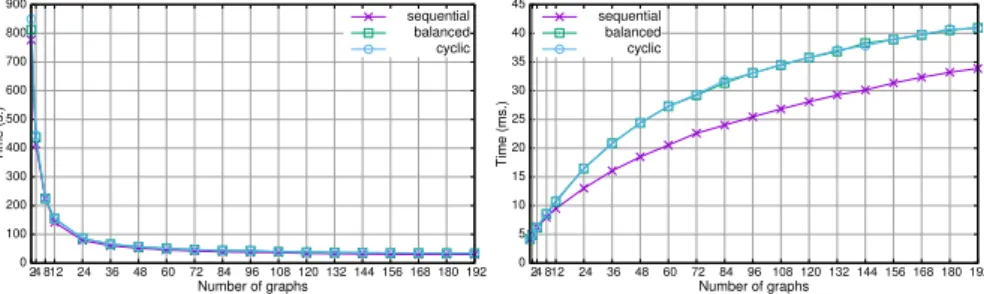
(8) 8. F.J. Artigas-Fuentes, J.M. Badı́a. where the cosine of the angle between the two vectors is computed as follows: Pn k=1 (vik ∗ vjk ) qP (2) cos(vi , vj ) = qP n n 2 )∗ 2 ) (v (v k=1 ik k=1 jk The experimental results were obtained on two different parallel platforms: hexa is a 16-node distributed memory cluster connected through a InfiniBand network, each node equipped with two Intel Xeon E5645 (hexacore) processors at 2.4 GHz and 24 GBytes of RAM. Therefore, we are using a total of 16 × 2 × 6 = 192 cores. sun is a shared memory multiprocessor Sun X4470 with 32 cores (64 logical cores exploiting hyper-threading). It includes 4 Intel Xeon X7550 processors at 20 GHz, each containing 8 cores and a total of 64 GBytes of RAM.. 6 Experimental analysis We have compared three different distributions of the objects of the Reuters repository among the graphs. First we distribute sequentially the objects of the repository in equal-sized blocks keeping the order given by the repository. Second, we distribute the objects in different-sized blocks but balancing the total number of terms in the vectors assigned to each processor. Finally, we distribute the objects cyclically among the processors in order to nullify any kind of topic clustering included in the original repository.. 6.1 Cost of the sequential access method. 900. 35. 600. 30. 500 400. 25 20. 300. 15. 200. 10. 100 0. sequential balanced cyclic. 40. 700. Time (ms.). Time (s.). 45. sequential balanced cyclic. 800. 5 24 812. 24. 36. 48. 60. 72. 84. 96 108 120 132 144 156 168 180 192. Number of graphs. 0. 24 812. 24. 36. 48. 60. 72. 84. 96 108 120 132 144 156 168 180 192. Number of graphs. Fig. 1 Cost to build the indexes (left) and average time per search (right) varying the number of graphs of the index with the three distributions of the objects among the graphs.. Our first set of experiments was performed in hexa with the sequential version to evaluate the cost of building our index structure. Figure 1.a shows the time required to generate the multiple graphs index with the Reuters.

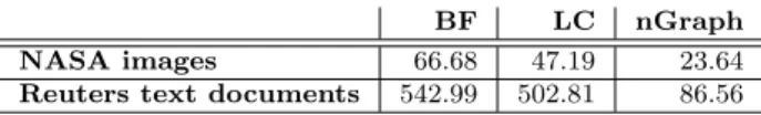
(9) Accessing very high dimensional spaces in parallel. 9. repository for a connectivity of δ = 5. The cost clearly decreases as we increase the number of graphs and reduce the number of objects per graph. The cost of building all the graphs decreases quadratically with the size of each graph and only increases linearly with the number of graphs. The distribution of the objects among the graphs affects only slightly the building cost. Figure 1.b shows the average time required to obtain the 1 − N N of a random set of 10,000 objects from the collection. As we increase the number of graphs we have to explore globally more entry points and, once we choose the nearest entry point to the query on each graph, we have to explore its neighborhood. The time increases almost linearly with a few graphs, but it clearly slows down as we distribute the object of the index in more graphs. We can process sequentially hundreds of queries per second with our sequential algorithm. However, we need to parallelize the search process to increase the throughput and to be able to process efficiently larger flows of queries. This figure also shows that the sequential distribution of the objects in the repository produces faster searches. This happens because in the Reuters repository the objects are sorted by topic. Therefore, most of the nearest neighbors to every query are included in one or a few graphs and the stopping condition is reached sooner in every other graph. The spatial cost of our index structure allows us to deal with millions of documents on the main memory of the processors, including both data and index. For example, storing 80,000 documents of the Reuters collection and building one graph takes 538 Mbytes, while building an index with 192 graphs takes 802 Mbytes. Increasing the minimum connection degree from 5 to 20 only increases the size to 851 Mbytes. This cost scales with the number of processes as we distribute the data and graphs among all of them. Finally, table 1 shows the sequential search cost of three methods obtained in a processor of sun with the two datasets to find the 8 kNN of every query. Our sequential algorithm using one graph (nGraph) clearly outperforms the brute force method (BF) and the method that uses an LC index, specially with very high dimensional text documents.. NASA images Reuters text documents. BF 66.68 542.99. LC 47.19 502.81. nGraph 23.64 86.56. Table 1 Sequential search time in seconds to process 23,381 image queries with an index of size 95,202 and 10,000 document queries with an index containing 60,000 documents.. 6.2 Quality of the search results In order to analyze de quality of the search process we compute the precision of our search results over the same set of 10,000 queries used on the previous section and relate it with the percentage of objects of the index visited. We.

(10) 10. F.J. Artigas-Fuentes, J.M. Badı́a. define the precision as the percentage of results of our method that correpond to the exact results of the query. We obtain the exact results by means of an exhaustive search that compares all the objects of the index with the query to find its 1 − N N .. Precision and Visited objects (%). 100 90 80 70 60 50 40. Prec. seq Prec. bal Prec. cyc Visi. seq Visi. bal Visi. cyc. 30 20 10 0. 24 812. 24. 36. 48. 60. 72. 84. 96 108 120 132 144 156 168 180 192. Number of graphs. Fig. 2 Percentage of visited objects and precision of the search results to find the 1-NN of 10,000 queries on Reuters repository.. Figure 2 shows the relationship between the precision of the results and the portion of the repository visited during searches. As we can see we obtain results with very high precision, i.e., it is always over 68% and tends to stabilize over 90% as we increase the number of graphs, even when the value of minimum connection degree of the graphs used is only 5. Besides, the quality of the results does not depend on the distribution of the objects among the graphs. We can also see that the percentage of visited objects grows with the number of graphs included on the index structure. When use few graphs (less than 24) most of the visited objects are entry points of the graphs, while more internal points are visited as we increase the number of graphs. On the other hand, a sequential distribution of the objects of the Reuters repository among the graph reduces the percentage of visited objects, and accordingly the search time (see Figure 1.b), as the pruning rule stops the search sooner in almost all graphs. 6.3 Parallel access method analysis In this section we use hexa to analyze the cost and speedup of our parallel methods for both the construction of index structure and search process using Reuters dataset. The speedups of the parallel algorithms are always obtained with respect to the sequential algorithm that uses the same index structure and obtains the same search results. That is, we compute the speedup of the parallel algorithms over p processors with respect to the sequential version of the algorithm building or searching sequentially the same p graphs in one processor..

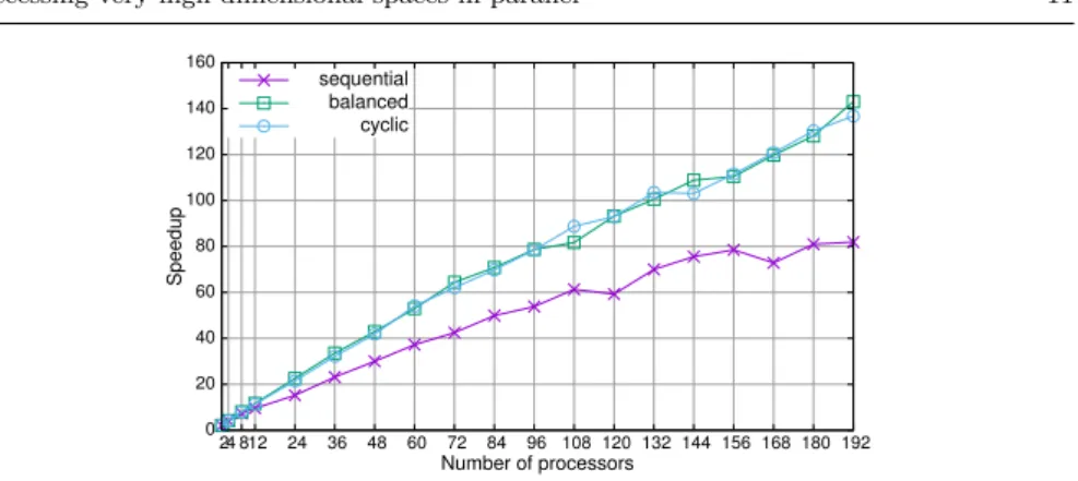
(11) Accessing very high dimensional spaces in parallel 160. 11. sequential balanced cyclic. 140. Speedup. 120 100 80 60 40 20 0. 24 812. 24. 36. 48. 60. 72. 84. 96 108 120 132 144 156 168 180 192. Number of processors. Fig. 3 Speedup of the parallel construction of the index structure.. Figure 3 shows that we obtain very good speedups with the parallel building algorithm. Recall that we are dealing with an embarrassingly parallel process that does not involve any kind of communication or synchronization among the processors. We are not obtaining optimal speedups due to the different cost of building each graph. The effect of this unbalanced cost is larger with a sequential distribution of the objects of the repository. 120. 120. sequential balanced cyclic. 100. 80. Speedup. Speedup. 80. 60. 60. 40. 40. 20. 20. 0. sequential balanced cyclic. 100. 24 812. 24. 36. 48. 60. 72. 84. 96 108 120 132 144 156 168 180 192. Number of processors. 0. 24 812. 24. 36. 48. 60. 72. 84. 96 108 120 132 144 156 168 180 192. Number of processors. Fig. 4 Speedup of the parallel search algorithms: master-slave (left) and pipeline (right).. Regarding the parallel search algorithms, Figure 4 lets us analyze and compare the behavior of the master-slave and the pipeline schemes. Both algorithms clearly reduce the cost of the sequential version. However, the pipeline algorithm is much more efficient than the master-slave algorithm. Two main factors define the speedup of both algorithms: the communication cost and the load balance. In the case of the master-slave algorithm we have to broadcast every query object to all the processors, perform the parallel search of all k neighbors and then gather and combine the local solutions on the master processor. Both communication stages involve a high percentage of the total cost of processing each query, thus reducing the speedup of the parallel process. Besides, as we process a flow of queries, both stages force two synchronization points for every query. As the processing time of each query is not perfectly balanced on.

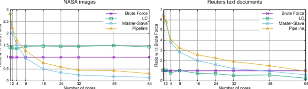
(12) 12. F.J. Artigas-Fuentes, J.M. Badı́a. the different processors, all processors have to wait to the slowest one before processing the next query. The pipeline scheme reduces the effect of the communication and unbalance problems. In this case we are only sending point to point messages between ’adjacent’ pairs of processors and there are not synchronization points imposed on all the processors by the communications. Therefore, as the queries flow through the pipeline, the communications can be overlapped with the processing of the queries, thus hiding part of the communication cost and reducing the effect of the load unbalance. However, as it happens with the master-slave scheme, in the case of the sequential distribution of the objects among the graphs, the cost of every search is always larger in the processors containing the documents of the same topic that the query, increasing the effect of the unbalance and producing worse speedups. In order to reduce even more the negative effect of the communication cost and load balance we have analyzed the effect of processing blocks of queries instead of individual queries. Grouping several queries increases the searching cost and reduces the weight of the communications. Besides, including queries with different search costs on each block usually balances the total cost of processing the different blocks. We compared our two parallel search algorithms with a parallel version of the search method that uses the LC index implemented using OpenMP [9] on shared memory multiprocessor sun. To assess the performance of the algorithms we took as reference an OpenMP parallel implementation of the brute force method. Both, the LC and brute force algorithms use a global index and apply inter-query parallelism without any kind of communication or synchronization among the threads. On the contrary, our two algorithms use a local index distributed among the cores. The master-slave algorithm uses intraquery parallelism applied to every query. The pipeline algorithm also applies inter-query parallelism, but starting one query after the other. NASA images. Reuters text documents Brute Force LC Master-Slave Pipeline. Ratio w.r.t Brute Force. 2.5 2 1.5 1 0.5 0. 7. Brute Force LC Master-Slave Pipeline. 6. Ratio w.r.t Brute Force. 3. 5 4 3 2 1. 12 4. 8. 16. 24. 32. Number of cores. 48. 64. 0. 12 4. 8. 16. 24. 32. 48. 64. Number of cores. Fig. 5 Search time ratio of the parallel algorithms with respect to the parallel brute force method with the two datasets.. Figure 5 compares the search time of the parallel algorithms with respect to the brute force method using both datasets. In the case of the NASA images with low dimensionality (D = 20), the best performances are obtained in most.

(13) Accessing very high dimensional spaces in parallel. 13. cases with the LC algorithm. Our parallel algorithms only outperform the LC algorithm when using a few threads. As we increase the number of threads and graphs in the index, the selectivity of our algorithm decreases (see Figure 2) while the communication cost increases. When applied to very high dimensional text documents the curse of dimensionality greatly affects the LC algorithm. It cannot discard any cluster while processing the queries and it has to compare every query with all the documents. As a result it obtains even worse results than the brute force algorithm. On the contrary, our parallel algorithms aren’t so affected by the high dimensionality of the documents. The pipeline algorithm outperforms the other parallel algorithms and equals the time of the brute force approach with 64 processes and graphs when it has lost selectivity and is more affected by the communications. 7 Conclusions This paper shows that it is possible to process efficiently large flows of queries on very high-dimensional objects in parallel. We have implemented a new access method based on the use of multiple graphs as an index whose construction and search can be naturally parallelized on shared and distributed memory multiprocessors. Besides, this new approximate access method produces high quality results with precisions larger than 90% when we increase the number of graphs of the index. Experimental results on real text document repositories show very large speedups both during the index construction and during the search process. A pipeline parallel scheme applied to the search process allows us to deal with tens of thousands of queries per second. When compared with a compact partitioning algorithm, we can see that our algorithms are not so affected by the curse of dimensionality when applied to very high dimensional documents. They clearly outperform other methods in the sequential case and obtain the best results in the parallel case.. 8 Acknowledgements This research has been supported by the CICYT project TIN2014-53495-R of the Ministerio de Economı́a y Competitividad.. References 1. Ares, L.G., Brisaboa, N.R., Pereira, A.O., Pedreira, O.: Efficient similarity search in metric spaces with cluster reduction. In: Similarity Search and Applications - 5th International Conference, SISAP 2012, Toronto, ON, Canada, August 9-10, 2012. Proceedings, pp. 70–84 (2012).

(14) 14. F.J. Artigas-Fuentes, J.M. Badı́a. 2. Artigas-Fuentes, F.J., Gil-Garcı́a, R., Badı́a-Contelles, J.M.: A high-dimensional access method for approximated similarity search in text mining. In: 20th International Conference on Pattern Recognition, ICPR 2010, Istanbul, Turkey, 23-26 August 2010, pp. 3155–3158 (2010) 3. Artigas-Fuentes, F.J., Gil-Garcı́a, R., Badı́a-Contelles, J.M., Pons-Porrata, A.: Fast k -nn classifier for documents based on a graph structure. In: Progress in Pattern Recognition, Image Analysis, Computer Vision, and Applications - 15th Iberoamerican Congress on Pattern Recognition, CIARP 2010, Sao Paulo, Brazil, November 8-11, 2010. Proceedings, pp. 228–235 (2010) 4. Aydin, B.: Parallel algorithms on nearest neighbor search. Survey paper. Georgia State University (2014) 5. Baeza-Yates, R.A., Ribeiro-Neto, B.A.: Modern Information Retrieval - the concepts and technology behind search, Second edition. Pearson Education Ltd., England (2011) 6. Barrientos, R.J., Gómez, J.I., Tenllado, C., Prieto-Matı́as, M., Marı́n, M.: knn query processing in metric spaces using gpus. In: Euro-Par 2011 Parallel Processing - 17th International Conference, Euro-Par 2011, Bordeaux, France, August 29 - September 2, 2011, Proceedings, Part I, pp. 380–392 (2011) 7. Barrientos, R.J., Gómez, J.I., Tenllado, C., Prieto-Matı́as, M., Marı́n, M.: Range query processing on single and multi GPU environments. Computers & Electrical Engineering 39(8), 2656–2668 (2013) 8. Chávez, E., Navarro, G.: A compact space decomposition for effective metric indexing. Pattern Recognition Letters 26(9), 1363–1376 (2005) 9. Costa, V.G., Barrientos, R.J., Marı́n, M., Bonacic, C.: Scheduling metric-space queries processing on multi-core processors. In: Proceedings of the 18th Euromicro Conference on Parallel, Distributed and Network-based Processing, PDP 2010, Pisa, Italy, February 17-19, 2010, pp. 187–194 (2010) 10. Costa, V.G., Marı́n, M.: Distributed sparse spatial selection indexes. In: 16th Euromicro International Conference on Parallel, Distributed and Network-Based Processing (PDP 2008), 13-15 February 2008, Toulouse, France, pp. 440–444 (2008) 11. Costa, V.G., Marı́n, M., Reyes, N.: Parallel query processing on distributed clustering indexes. J. Discrete Algorithms 7(1), 3–17 (2009) 12. Dashti, A.: Efficient computation of k-nearest neighbor graphs for large highdimensional data sets on gpu clusters. Master’s thesis, University of WisconsinMilwaukee, Paper 280 (2013) 13. Dong, W.: High-dimensional similarity search for large datasets. Ph.D. thesis, Department of Computer Science, Princeton University (2011) 14. Garcia, V., Nielsen, F.: Searching high-dimensional neighbours: CPU-based tailored data-structures versus GPU-based brute-force method. In: MIRAGE. 4th International Conference on Computer Vision/Computer Graphics Collaboration Techniques, pp. 425–436 (2009) 15. Kamble, A.: Survey of text categorization techniques. IJRCCT 3(7) (2014) 16. Lewis, D.D., Yang, Y., Rose, T.G., Li, F.: RCV1: A new benchmark collection for text categorization research. Journal of Machine Learning Research 5, 361–397 (2004) 17. Marı́n, M., Reyes, N.: Efficient parallelization of spatial approximation trees. In: Computational Science - ICCS 2005, 5th International Conference, Atlanta, GA, USA, May 22-25, 2005, Proceedings, Part I, pp. 1003–1010 (2005) 18. Marı́n, M., Uribe, R., Barrientos, R.J.: Searching and updating metric space databases using the parallel EGNAT. In: Computational Science - ICCS 2007, 7th International Conference Beijing, China, May 27-30, 2007, Proceedings, Part I, pp. 229–236 (2007) 19. Naidan, B., Boytsov, L., Nyberg, E.: Permutation search methods are efficient, yet faster search is possible. PVLDB 8(12), 1618–1629 (2015) 20. Pan, J., Manocha, D.: Fast gpu-based locality sensitive hashing for k-nearest neighbor computation. In: 19th ACM SIGSPATIAL International Symposium on Advances in Geographic Information Systems, ACM-GIS 2011, November 1-4, 2011, Chicago, IL, USA, Proceedings, pp. 211–220 (2011) 21. Paredes, R.: Graph for metric space searching. Ph.D. thesis, Universidad de Chile (2008) 22. Radovanovic, M., Nanopoulos, A., Ivanovic, M.: Hubs in space: Popular nearest neighbors in high-dimensional data. J Mach Learn Res 11, 2487–2531 (2010).

(15)