Scalable RDF compression with MapReduce and HDT

U

NIVERSIDAD DE

V

ALLADOLID

E

T

S

I

T

T

RABAJO

F

IN DE

M

ASTER

M

U

I

EN

T

I

C

Scalable RDF compression

with MapReduce and HDT

Autor:

D. José Miguel Giménez García

Tutores:

Dr. D. Pablo de la Fuente

Dr. D. Miguel A. Martínez-Prieto

Dr. D. Javier D. Fernández

with MapReduce and HDT

AUTOR:

D. José Miguel Giménez García

TUTORES:

Dr. D. Pablo de la Fuente

Dr. D. Miguel A. Martínez-Prieto

Dr. D. Javier D. Fernández

DEPARTAMENTO:

Departamento de Informática

Tribunal

PRESIDENTE:

Dr. D. Carlos Alonso González

VOCAL:

Dr. D. Mercedes Martínez

SECRETARIO:

Dr. D. Arturo González Escribano

FECHA:

11 de septiembre de 2015

CALIFICACIÓN:

Resumen del TFM

El uso de RDF para publicar datos semánticos se ha incrementado de forma notable en los últimos años. Hoy los datasets son tan grandes y están tan interconectados que su procesamiento presenta problemas de escalabilidad. HDT es una representación compacta de RDF que pretende minimizar el consumo de espacio a la vez que proporciona capacidades de consulta. No obstante, la generación de HDT a partir de formatos en texto de RDF es una tarea costosa en tiempo y recursos. Este trabajo estudia el uso de MapReduce, un framework para el procesamiento distribuido de grandes cantidades de datos, para la tarea de creación de estructuras HDT a partir de RDF, y analiza las mejoras obtenidas tanto en recursos como en tiempo frente a la creación de dichas estructuras en un proceso mono-nodo.

Palabras clave

Big Data, HDT, MapReduce, RDF, Web Semántica.

Abstract

The usage of RDF to expose semantic data has increased dramatically over the recent years. Nowadays, RDF datasets are so big and interconnected their management have significant scalability problems. HDT is a compact representation of RDF data aiming to minimize space consumption while providing retrieval features. Nonetheless, HDT generation from RDF traditional formats is expensive in terms of resources and processing time. This work introduces the usage of MapReduce, a framework for distributed processing of large data quantities, to serialize huge RDF into HDT, and analyzes the improvements in both time and resources against the prior mono-node processes.

Keywords

Agradecimientos

Me gustaría expresar mi agradecimiento a varias personas, sin las cuales este trabajo no hubiera sido posible, o hubiera sido muy diferente.

En primer lugar a mis tutores, Javier D. Fernández, Miguel A. Martínez-Prieto, y Pablo de la Fuente, por su ayuda e infinita pacienca durante la realización del trabajo.

A Javier I. Ramos, por su apoyo constante con el cluster Hadoop, en especial cuando hubo problemas que hacían que el sistema de virtualización fallase.

A Jurgen Umbrich, por prestar el servidor en el que se realizaron las pruebas mono-nodo de

hdt-lib.

A Mercedes Martínez y Diego Llanos. Trabajos realizados en sus asignaturas sirvieron de inspiración para lo que más tarde se convirtió en parte de esta memoria.

A mí familia, que como siempre han estado dándome su apoyo, estuvieran o no de acuerdo con mis decisiones.

A mis amigos, que siempre me han dado ánimos para continuar.

Contents

1 Introduction 1

1.1 Motivation . . . 1

1.2 Goals . . . 2

1.3 Methodology . . . 4

1.4 Structure . . . 4

2 Background 5 2.1 Semantic Web . . . 5

2.1.1 Foundations of the Semantic Web . . . 5

2.1.2 Scalability Challenges . . . 16

2.2 HDT . . . 17

2.2.1 Structure . . . 17

2.2.2 Building HDT . . . 18

2.2.3 Performance . . . 19

2.2.4 Scalability Issues . . . 19

2.3 MapReduce . . . 19

2.3.1 Distributed FileSystems . . . 20

2.3.2 MapReduce . . . 23

2.3.3 Challenges and Main Lines of Research . . . 26

3 State of the Art 31 3.1 SPARQL Query Resolution . . . 31

3.1.1 Native solutions . . . 33

3.1.2 Hybrid Solutions . . . 37

3.1.3 Analysis of Results . . . 40

3.2 Reasonig . . . 42

3.3 RDF Compression . . . 45

3.4 Discussion . . . 46

4 HDT-MR 49 4.1 System Design . . . 49

4.1.1 Process 1: Dictionary Encoding . . . 49

4.1.2 Process 2: Triples Encoding . . . 52

4.2 Implementation and configuration details . . . 54

4.2.1 Job 1.1: Roles Detection . . . 55

4.2.2 Job 1.2: RDF Terms Sectioning . . . 55

4.2.3 Local sub-process 1.3: HDT Dictionary Encoding . . . 56

4.2.4 Job 2.1: ID-triples serialization . . . 57

4.2.5 Job 2.2: ID-triples Sorting . . . 57 4.2.6 Local sub-process 2.3: HDT Triples Encoding . . . 57

5 Experiments and Results 61

6 Conclusions and Future Work 67

6.1 Conclussions . . . 67 6.2 Future Work . . . 67 6.3 Contributions and Publications . . . 68

A HDT-MR parameters 79

B HDT-MR configuration files 83

List of Figures

1.1 Goals overview . . . 3

2.1 Semantic Web Architecture . . . 6

2.2 An RDF graph example . . . 8

2.3 An RDFS graph example . . . 9

2.4 A SPARQL query example . . . 13

2.5 RDFS inference rules . . . 15

2.6 OWL Horst inference rules . . . 15

2.7 LOD Cloud (as of August 2014) . . . 16

2.8 HDT Dictionary and Triples configuration for an RDF graph . . . 18

2.9 Distributed File System Architecture (HDFS) . . . 21

2.10 Distributed File System Write Dataflow . . . 22

2.11 Map and Reduce input and output . . . 23

2.12 MapReduce Architecture Overview . . . 24

2.13 Complete MapReduce Dataflow . . . 25

2.14 Map, Combine and Reduce inputs and outputs . . . 25

3.1 Example of different hop partitions . . . 39

3.2 RDFS rules ordering . . . 43

3.3 Compression and decompression algorithms . . . 47

4.1 HDT-MR workflow. . . 49

4.2 Example of Dictionary Encoding: roles detection (Job 1.1). . . 50

4.3 Example of Dictionary Encoding: RDF terms sectioning (Job 1.2). . . 52

4.4 Example of Triples Encoding: ID-triples Serialization (Job 2.1). . . 53

4.5 Example of Triples Encoding: ID-triples Sorting (Job 2.2) . . . 54

4.6 Class Diagram: Job 1.1: Roles Detection . . . 55

4.7 Class Diagram: Job 1.2: RDF Terms Sectioning . . . 56

4.8 Class Diagram: Job 2.1: ID-triples serialization . . . 57

4.9 Class Diagram: Local sub-process 2.3: HDT Triples Encoding . . . 59

5.1 Serialization times: Real-World Datasets . . . 63

5.2 Serialization times: LUBM (1) . . . 63

5.3 Serialization times: LUBM (2) . . . 64

5.4 Serialization times: LUBM vs SP2B . . . 64

List of Tables

3.1 MapReduce-based solutions addressing SPARQL resolution . . . 32

4.1 Cluster configuration. . . 54

5.1 Experimental setup configuration. . . 61

5.2 Statistical dataset description . . . 62

5.3 Statistical dataset description of SP2B and LUBM . . . 64

Chapter 1

Introduction

1.1

Motivation

Since the end of the last century, the volume of data generated and stored across information systems has been growing at a dramatic rate. The estimated amount of data of the digital universe was 281 exabytes (281 billion gigabytes) in 2006 [42], and reached 1.8 zettabytes (1.8 trillion gigabytes) in 2011 [41], multiplying its volume by six in five years. In addition, most of these data, ranging from health records to twitter feeds, is not stored in structured format [9].

The so called Data Deluge affects a myriad of fields. In scientific research, large amounts of data are collected from simulations, experimental results, and even observation devices such as telescopes: The Murchison Widefield Array (MWA) —a radio telescope based in Western Australia’s Mid West— is currently generating 400 megabytes of data per second (33 terabytes per day) [17]. Internet companies like Google, Facebook or Yahoo! have stored data measured in exabytes [111]. Public administrations have released millions of datasets to the public under the Open Government flag [55].

However, management of Big Data presents some challenges. The more important among them are related to what are commonly known as “the three V’s of Big Data”:

• Variety: As said before, Big Data are generated by a multitude of sources. The structure of all this data is heterogeneous, and in many cases data are not even structured at all. Because of this, extracting information and establishing relations among data is difficult.

• Volume: Probably the most straightforward challenge, the sheer amount of data is a problem by itself. Storage, transmission or querying of information cannot be addressed by classical IT technologies.

• Velocity: Data are generated at an increasingly rapid rate. Processing the information quickly enough is an added issue when dealing with Big Data.

The Semantic Web [7] is a solution that attempts to deal with the challenge of Variety. In short, it is a proposal with the initial purpose of transforming the current web into a Web of Data, where semantic content is exposed and interlinked instead of plain documents. To allow a standardized way to represent semantic data, the Resource Description Framework (RDF) [4] is introduced by the W3C. RDF represents data in a labeled directed graph structure, enabling heterogeneous data to be linked in a uniform way, while endowing links with semantic meaning.

The Semantic Web has provided means for publication, exchange and consumption of Big Semantic Data. Since its inception, RDF usage has grown exponentially, with datasets spanning hundreds of millions triples. Nonetheless, managing those quantities of data is still a challenge.

While different approaches have been proposed, such as column-oriented databases [109], Velocity and Volume are still unresolved challenges.

To address the Velocity issues that the Semantic Web struggles with, it is necessary a way to transmit and query RDF in an efficient way. HDT is a storage proposal for RDF storage based on succinct data structures [36] to confront scalability problems in the publication, exchange and consumption cycle of Semantic Data. HDT is currently a W3C Member Submission1

RDF storage, transmission and querying requirements are alleviated by HDT. However, this comes with a price. Current methods of serializing RDF into HDT need to process the whole RDF dataset, demanding high amounts of memory in order to manage intermediate data structures. That is, scalability issues are moved from RDF consumption to HDT generation. Volume is then an issue that RDF serialization into HDT has still to face.

In this scenario, MapReduce emerges as a candidate for this process. In short, MapReduce is a framework for distributed processing of large amounts of data over commodity hardware. It is based on two main operations: Map, which gathers information items in the form of pairs key-value, andReduce, which groups values with the same key. Originally developed by Google and made public in 2004 [27], its usage took off since then and it is currently widely used by many institutions and companies, such as Yahoo! [108], Facebook [117] or Twitter [75].

1.2

Goals

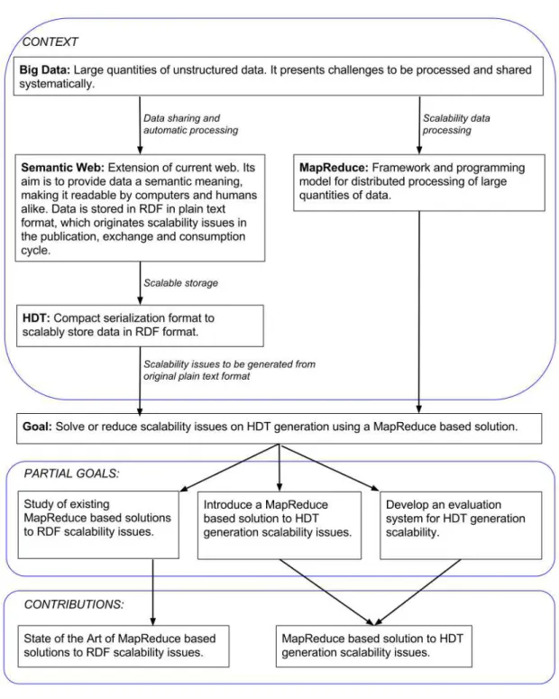
The main goal for this work is to address the scalability issues of HDT serialization using the MapReduce framework, reducing hardware requirements to generate an HDT serialization from massive datasets or mashups. In order to achieve this objective some intermediate or secondary goals are introduced. Those goals are sketched, along with a context overview, in Figure 1.1. They are also described below.

• Perform a study of existing MapReduce based solutions to RDF scalability issues.

• Devise a MapReduce based solution to HDT serialization scalability issues. This solution has to address the generation of the two serialized components of HDT, each one presenting a different challenge:

– Dictionary serialization. Every triple term must be identified, segregated into sections

according to its role, and assigned a unique and ascending numerical IDs. Here the challenge is to segregate and sort the terms, considering that terms which are subjects and objects simultaneously belong to a different section than terms that are just subjects or objects. This process is currently being done using temporal in-memory structures, and constitutes the main bottleneck of HDT serialization.

– Triples serialization. Every triple term must be substituted by its ID. Then, each triple

must be identified and sorted by subject, predicate and object. While here there are no hardware requirements that make the task unrealizable, speed can be improved by paralleling the operation.

• Develop an evaluation system for HDT generation scalability. This system will have to be applied to the devised solution and provide an unbiased assessment of its scalability, comparing it with previous mono-node versions.

1

1.2. GOALS 3

1.3

Methodology

This work proposes a novel approach to deal with HDT serialization, which is in itself a solution to deal with RDF scalability issues. This is a multidisciplinary work on the fields of Semantic Web, compression techniques, and parallel computation, so a preliminary study of all fields is very important. This allows to fully understand the subject and to take a grasp of useful techniques, possible issues, and solutions on applying the MapReduce model to deal with RDF and HDT structures. This is visible in the used methodology, which comprises the following steps:

1. Perform a state-of-the-art of Semantic Web, HDT and MapReduce, describing its main characteristics, strengths, weaknesses and current challenges and lines of research.

2. Analyze current MapReduce-based solutions on the Semantic Web regarding scalability issues.

3. Propose and develop a solution to HDT scalability issues. This solution will be based on the MapReduce computational model.

4. Evaluate the solution against the previous mono-node serialization algorithm, providing a fair assessment of the applicability of the devised solution.

1.4

Structure

The current chapter provides an overview of the problem this work addresses, its goals and methodology. The rest of this document is organized as follows:

• Chapter 2 describes the background regarding the Semantic Web, HDT and MapReduce. • Chapter 3 reviews the most relevant MapReduce solutions to a variety of RDF scalability

issues, not only including compression, but also query resolution and inference issues. • Chapter 4 describes the proposed solution to generate HDT serialization. The evaluation

method for this solution is also defined.

• Chapter 5 demonstrates the experiments and their results with real-world and synthetic datasets.

Chapter 2

Background

This chapter explores the background needed to understand the addressed problem. This back-ground includes the foundations and challenges of the Semantic Web and a description of the MapReduce framework, on which HDT-MR is based upon.

2.1

Semantic Web

This section describes the basics of the Semantic Web: its principles, foundations, and standards. It also comments its current challenges and open fields of research.

2.1.1 Foundations of the Semantic Web

The foundations of the Semantic Web are based on the current World Wide Web. In the WWW the information is published and consumed by a multitude of different actors. Information is published as documents, interconnected by links, and can be viewed as a whole as a directed graph. In this graph, each document is a edge, while each link is a vertex. Then, information is presented in natural language [7], and meaning is inferred by people who read web pages and the labels of hyperlinks [98]. In the current web there are huge quantities of data, but utilization is limited due to inherent problems [24]:

• Information overload: Information on the web grows rapidly and without organization, so it is difficult to extract useful information from it.

• Stovepipe Systems: Many information system components are built to work only with another components of the same system. Information from these components is not readable by external systems.

• Poor Content Aggregation: The Web is full of disparate content which is difficult to aggregate. Scraping is the common solution.

The Semantic Web was first proposed by Tim Berners-Lee [7] in 2001. It expands the concept of organizing information as a directed graph, but instead of linking documents, it links semantic data. The links have also semantic labels, in order to describe the relation between the two entities. Its goal is to make data discoverable and consumable not only by people, but also by automatic agents [98]. It is based on the following foundations [7, 98]:

• Resources: A resource is intended to represent any idea that can be referred to, whether it is actual data, just a concept, or a reference to a real or fictitious object.

• Standardized addressing: All resources on the Web are referred to by URIs [8]. The most familiar URIs are those that address resources that can be addressed and retrieved; these are called URLs, for Uniform Resource Locators.

• Small set of commands: The HTTP protocol [38] (the protocol used to send messages back and forth over the Web) uses a small set of commands. These commands are universally understood.

• Scalability and large networks: The Web has to operate over a very large network with an enormous number of web sites and to continue to work as the network’s size increases. It accomplishes this thanks to two main design features. First, the Web is decentralized. Second, each transaction on the Web contains all the information needed to handle the request.

• Openness, completeness, and consistency: The Web is open, meaning that web sites and web resources can be added freely and without central controls. The Web is incomplete, meaning there can be no guarantee that every link will work or that all possible information will be available. It can be inconsistent: Anyone can say anything on a web page, so different web pages can easily contradict each other.

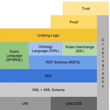
Figure 2.1: Semantic Web Architecture

2.1. SEMANTIC WEB 7 • XML —Extensible Markup Language [14]: Language framework that lets write structured Web documents with a user-defined vocabulary. Since 1998, it has been used to define nearly all new languages that are used to interchange data over the Web.

• XML Schema [34, 114, 11]: A language used to define the structure of specific XML languages.

• RDF —Resource Description Framework [74]: A flexible language capable of describing information and meta data. The RDF data model does not rely on XML, but RDF has an XML-based syntax. RDF is covered in section 2.1.1.1

• RDF Schema [15]: A framework that provides a means to specify basic vocabularies for specific RDF application languages to use. It provides modeling primitives for organizing Web objects into hierarchies. Key primitives are classes and properties, subclass and sub-property relationships, and domain and range restrictions. RDF Schema is covered in 2.1.1.2.

• Ontology–Languages: Expand RDF Schema to allow definition of vocabularies and estab-lish the usage of words and terms in the context of a specific vocabulary. RDF Schema is a framework for constructing ontologies and is used by many more advanced ontology frame-works. OWL [50] is an ontology language designed for the Semantic Web. Section 2.1.1.3 discusses OWL.

• Logic and Proof : Logical reasoning is used to establish the consistency and correctness of datasets and to infer conclusions that aren’t explicitly stated but are required by or consistent with a known set of data. Proofs trace or explain the steps of logical reasoning. Section 2.1.1.5 covers some issues relating to logic in the Semantic Web.

• Trust: A mean of providing authentication of identity and evidence of the trustworthiness of data, services, and agents.

2.1.1.1 RDF

RDF is a data model to describe resources, where a resource can be anything in principle. It proposes a date model based on making statements about the resources. Each statement has then the structure of a triple with the following components [24]:

• Subject: The resource that is being described by the ensuing predicate and object. A subject can be either an IRI or a blank node.

• Predicate: The relation between the subject and the object. A predicate is an IRI.

• Object: Either a resource or value referred to by the predicate. An object can be an IRI, a blank node, or a literal.

An IRI (International Resource Identifier) [30] refers unequivocally to a single resource. IRIs are a generalization of an URIs that can contain characters from the Universal Character Set. RDF has rules about how to construct an URI from an IRI so that they can be used conveniently on the Word Wide Web [98]. Blank nodes are local identifiers that are often used to group collections of resources, while a literal is a text string, commonly used for names or descriptions.

Definition 1 (RDF triple) A tuple(s, p, o) ∈ (I∪B) ×I× (I∪B∪L)is called an RDF triple, in which “s” is the subject, “p” the predicate and “o” the object.I (RDF IRI references),B(Blank nodes), andL(RDF literals) are infinite, mutually disjoint sets.

Definition 2 (RDF graph) An RDF graphGis a set of RDF triples. As stated,(s, p, o)can be represented as a directed edge-labeled graphsÐ→p o.

RDF Graph

ex:S1 foaf:age 25 . ex:S2 foaf:age 25 . ex:S1 ex:study ex:C1 . ex:S2 ex:study ex:C1 . ex:C1 ex:hasProfessor ex:P1 .

ex:S1

ex:hasProfessor

ex:S2

25 ex:C1 ex:P1

Figure 2.2: An RDF graph example

RDF is more redundant than other ways of storing information —as regular databases— because is schema-less. So, it needs to store property specifications each time they are used. This requires RDF to carry data that might otherwise be redundant [98]. But this trade-off between regularity and flexibility lets RDF do some operations that would be impossible in a conventional database, such as [98]:

• Combine the data with other datasets that do not follow the same data model.

• Add more data that does not fit the table structures.

• Exchange data with any other application that knows how to handle RDF. It can be done over the Web, by email, or any other way by which you can exchange a data file.

• Use an RDF processor that can do logical reasoning to discover unstated relationships in the data.

• Use someone else’s ontology to learn more about the relationships between the properties and resources in data.

• Add statements about publications and references that have been defined somewhere else on the Web. All that needs to be done is to refer to the published identifiers (URIs).

• Do all these things using well-defined standards, so that a wide range of software can process the data.

2.1. SEMANTIC WEB 9

2.1.1.2 RDF Schema

RDF Schema (or RDFS in short) defines classes and properties, using the RDF data model. Those elements allow to describe vocabularies (i.e. basic ontologies) to structure RDF resources and impose restrictions on what can be stated in an RDF dataset. A continuation of the RDF graph running example with some RDFS statements added is shown on Figure 2.3 The main elements of RDFS are outlined below [2].

RDF Graph

ex:Student rdf:type rdfs:Class . ex:Professor rdf:type rdfs:Class . ex:Class rdf:type rdfs:Class .

ex:S1 rdf:type ex:Student ex:S2 rdf:type ex:Student ex:P1 rdf:type ex:Professor ex:C1 rdf:type ex:Class

ex:S1 foaf:age 25 . ex:S2 foaf:age 25 . ex:S1 ex:study ex:C1 . ex:S2 ex:study ex:C1 . ex:C1 ex:hasProfessor ex:P1 .

ex:hasProfessor

ex:S2

25 ex:C1 ex:P1

ex:S1

ex:Professor ex:Class

ex:Student

rdfs:Class

rdf:type rdf:type rdf:type

rdf:type rdf:type

rdf:type

rdf:type

Figure 2.3: An RDFS graph example

Core Classes of RDFS:

• rdfs:Resource, the class of all resources.

• rdfs:Class: An element that defines a group of related things that share a set of properties [24]. It is the superclass of all classes.

• rdfs:Literal, the class of all literals (strings). At present, literals form the only data type of RDF/RDFS.

• rdf:Property, the class of all properties.

• rdf:Statement, the class of all reified statements.

Core Properties for Defining Relationships:

• rdf:type, which relates a resource to its class. The resource is declared to be an instance of that class.

• rdfs:subClassOf, which relates a class to one of its superclasses; all instances of a class are instances of its superclass. An element that specifies that a class is a specialization of an existing class. This follows the same model as biological inheritance, where a child class can inherit the properties of a parent class. The idea of specialization is that a subclass adds some unique characteristics to a general concept.

Core Properties for Restricting Properties:

• rdfs:domain, which specifies the domain of a property P, that is, the class of those resources that may appear as subjects in a triple with predicate P. If the domain is not specified, then any resource can be the subject.

• rdfs:range, which specifies the range of a property P, that is, the class of those resources that may appear as values in a triple with predicate P.

RDFS also includes utility properties to establish generic relations between resources or provide information to human readers, such as rdfs:seeAlso, rdfs:isDefinedBy,

rdfs:comment, andrdfs:label[2]

2.1.1.3 Ontologies and OWL

An ontology defines the common words and concepts (i.e. the meaning) used to describe and represent an area of knowledge [24]. An ontology language allows to model the vocabulary and meaning of domains of interest: the objects in domains; the relationships among those objects; the properties, functions, and processes involving those objects; and constraints on and rules about those things [24]. While RDF Schema provides some tools to do so, they are limited to a subclass hierarchy and a property hierarchy, with domain and range definitions of these properties [2]. The following requirement should be followed by a complete ontology language [2]:

• A well-defined syntax: A necessary condition for machine-processing of information • A formal semantics: Describes the meaning of knowledge precisely. Precisely here means

that the semantics does not refer to subjective intuitions, nor is it open to different interpre-tations.

• Efficient reasoning support: Allows to check the consistency of the ontology and the knowledge, check for unintended relationships between classes, and automatically classify instances in classes

• Sufficient expressive power: Needed to represent ontological knowledge. • Convenience of expression.

In detail, RDFS lacks expressive power to model an ontology because:

• Local scope of properties: rdfs:range defines the range of a property, say eats, for all classes. Thus in RDF Schema we cannot declare range restrictions that apply to some classes only. • Disjointness of classes: Sometimes we wish to say that classes are disjoint. For example,

male and female are disjoint. But in RDF Schema we can only state subclass relationships, e.g., female is a subclass of person.

• Boolean combinations of classes: Sometimes we wish to build new classes by combining other classes using union, intersection, and complement. For example, we may wish to define the class person to be the disjoint union of the classes male and female. RDF Schema does not allow such definitions.

2.1. SEMANTIC WEB 11 • Special characteristics of properties: Sometimes it is useful to say that a property is transitive (like “greater than”), unique (like “is mother of”), or the inverse of another property (like “eats” and “is eaten by”).

In order to achieve the expressive power that RDFS lacks the W3C developed OWL, an extension of RDF to describe ontologies. In OWL2, there are 3 OWL profiles, based on different description logics, with some trade-off between expressive power and efficiency of reasoning [92]: • OWL2-EL: Tailored for applications that need to create ontologies with very large number of classes and/or properties (as in large science ontologies). It is the profile with more expressive power, allowing classes to be defined with complex descriptions.

• OWL2-QL: Aimed at applications that use very large volumes of instance data, and where query answering is the most important reasoning task. Its goal is to allow reasoning to be translated into queries on a database. In order for reasoning to be translated into a query, its expressivity is restricted.

• OWL2-RL: Designed for applications that want to describe rules in ontologies. It is essentially a rules language for implementing logic in the form of rules if-then.

The main elements of OWL are described below [2].

Class Elements allow to declare and define classes with relation to another classes. • owl:Class: Defines a class.

• owl:disjointWith: To say that a class is disjoint with the specified class.

• owl:equivalentClass: To indicate that a class is equivalent with the specified class.

Property Elements allow to declare and define properties with relation to another properties. • owl:DatatypeProperty: Defines a data type property (a property that relates objects

with data type values).

• owl:ObjectProperty: Defines a object property (a property that relates objects with objects).

• owl:equivalentProperty: To indicate a equivalent class, with the same range and domain.

• owl:inverseOf: To say a property is inverse of the specified property (i.e. uses its range as domain, and its domain as range).

Property Restrictions allow to place property restrictions on defined classes.

• owl:Restriction: Specifies property restrictions on any class. Property restriction must be located betweenowl:Restrictiontags inside a class.

• owl:onProperty: Indicates the property that will be affected by the restriction.

• owl:hasValue: Specifies a fixed value that the property will have.

• owl:someValuesFrom: Makes mandatory to have at least one property with a value from the specified class. If the class has more than one of these properties, the rest are not restricted in this way.

• owl:minCardinality: Specifies the minimum cartinality of the property. • owl:maxCardinality: Specifies the maximum cartinality of the property.

Special Properties allow to define directly some attributes of property elements.

• owl:TransitiveProperty defines a transitive property, such as “has better grade than”, “is taller than”, or “is ancestor of”.

• owl:SymmetricPropertydefines a symmetric property, such as “has same grade as” or “is sibling of”.

• owl:FunctionalProperty defines a property that has at most one value for each object, such as “age”, “height”, or “directSupervisor”.

• owl:InverseFunctionalProperty defines a property for which two different ob-jects cannot have the same value, for example, the property “isTheSocialSecurityNumber-for” (a social security number is assigned to one person only).

Boolean Combinations allow to specify boolean combinations of classes.

• owl:complementOf: Specifies that the class is disjoint with the specified class. It has the same effect asowl:disjointWith.

• owl:unionOf: Specifies that the class is equal to the union of specified classes.

• owl:intersectionOf: Specifies that the class is equal to the intersection of specified classes.

Enumerations allow to define a class by listing all its elements. • owl:oneOf: Is used to list all elements that comprise a class.

Versioning information gives information that has no formal model-theoretic semantics but can be exploited by human readers and programs alike for the purposes of ontology management.

• owl:priorVersion: Indicate earlier versions of current ontology.

• owl:versionInfo: Contains a string giving information about the current ontology version.

• owl:backwardCompatibleWith: Identifies prior versions of the current ontology that are compatible with.

2.1. SEMANTIC WEB 13 Instances of OWL classes are declared as in RDF. OWL does not assume that instances with different name or ID are not the same instance (i.e. does not adopt the unique-names assumption). In order to ensure that resources are considered different from each other, this elements must be used:

• owl:differentFrom: Identifies the resource as different from the specified resource. • owl:AllDifferent: Allows to specify a collection. All elements of the collection are

considered different from each other.

2.1.1.4 SPARQL

Previous sections described how data are stored. As with traditional databases, it is necessary a way to inquire about the information contained in a dataset. SPAQRQL is the query language for the Semantic Web proposed by the W3C. SPARQL syntax is based on Turtle [5].

SPARQL is essentially a declarative language based on graph-pattern matching with a SQL-like syntax. Graph patterns are built on top of Triple Patterns (TPs), i.e., triples in which each of the subject, predicate and object may be a variable. These TPs are grouped within Basic Graph Patterns (BGPs), leading to query subgraphs in which TP variables must be bounded. Thus, graph patterns commonly join TPs, although other constructions, such as alternative (union) and optional patterns, can be specified in a query [30]. An SPARQL query example is presented on Figure 2.4. We can formally define TPs and BGPs as follows:

Definition 3 (SPARQL triple pattern) A tuple from(I∪L∪V) × (I∪V) × (I∪L∪V)is a triple pattern.

Note that blank nodes act as non-distinguished variables in graph patterns [100].

Definition 4 (SPARQL Basic Graph pattern (BGP)) A SPARQL Basic Graph Pattern (BGP) is

defined as a set of triple patterns. SPARQL FILTERs can restrict a BGP. IfB1is a BGP andRis

a SPARQL built-in condition, then(B1FILTERR)is also a BGP.

TP1

TP2 TP3 TP TP5

SP

QL Q

S

rdf:type ex:student . rdf:type ex:degree . ex:study .

ex:hasProfessor . rdf:type ex:professor

ex:student ex:de ree

ex: ofessor

rdf:type

rdf:type rdf:type ex:study

ex:hasProfessor

Figure 2.4: A SPARQL query example

Query resolution performance mainly depends on two factors:

1. Triples retrieval, which depends on how triples are organized and indexed.

Both concerns are typically addressed within RDF storage systems (RDF stores), which are usually built on top of relational systems or carefully designed from scratch to fit particular RDF peculiarities.

SPARQL allows to enquire information with four different statements:

• SELECT: Used to extract values.

• CONTRUCT: Used to extract information as RDF text. • ASK: Used to obtain yes/no questions.

• DESCRIBE: Used to extract arbitrary “useful” information.

A WHERE block is added (mandatory except in the case of DESCRIBE) where graph patterns to be matched are included.

2.1.1.5 Reasoning

RDF allows for inference of new knowledge not previously stated on the original data by using entailment rules. An entailment rule can be seen as a left-to-right rules: If the original data comply with the left side, the conclusion is added to the graph. ter Horst [113] describes entailment rules for RDFS and a subset of OWL (which serve as a basis for OWL2 RL definition), which can be seen in Figures 2.5 and 2.6, respectively.

There are two main approaches to perform inference: The first one consist of applying the rules at query time. In that case, the information related to the query is derived using backward-chaining reasoning. The second approach computes what is called the Graph Closure, applying all the entailment rules using forward-chaining reasoning, deriving and storing all the implicit information. Both approaches have advantages and disadvantages. The main advantage of the reasoning at query time is that it doesn’t require neither expensive precomputation nor space consumption. Thus, it is more suitable to datasets with dynamic information. However, the computations needed to perform the reasoning at query time are usually too expensive to be used in interactive applications. The computation of the Graph Closure, on the other hand, have the advantage of not needing any additional computation at query time. While this approach is suited for interactive applications, it is not efficient when only a small portion of the derivation is useful at query time.

2.1.1.6 Linked Data

Linked Open Data1 is a movement that advocates the publication of data under open licenses, promoting reuse of data for free. The project’s original and ongoing goal is to leverage the WWW infrastructure to publish and consume RDF data, achieving ubiquitous and seamless data integration over the WWW infrastructure [35]. This is accomplished by identifying existing datasets that are available under open licenses, converting them to RDF according to the Linked Data principles, and publishing them on the Web [12].

In 2006, Berners-Lee [6] enumerated the four principles the Web of Linked Data should follow in order to make possible for different datasets to be published on the current WWW infrastructure and connected together:

1. Use URIs as names for things. This allows any entity to be unambiguously referenced.

1

2.1. SEMANTIC WEB 15

1: s p o (if o is a literal) ⇒_:n rdf:type rdfs:Literal

2: p rdfs:domain x & s p o ⇒s rdf:type x

3: p rdfs:range x & s p o ⇒o rdf:type x

4a: s p o ⇒s rdf:type rdfs:Resource

4b: s p o ⇒o rdf:type rdfs:Resource

5: p rdfs:subPropertyOf q & q rdfs:subPropertyOf r ⇒p rdfs:subPropertyOf r

6: p rdf:type rdf:Property ⇒p rdfs:subPropertyOf p

7: s p o & p rdfs:subPropertyOf q ⇒s q o

8: s rdf:type rdfs:Class ⇒s rdfs:subClassOf rdfs:Resource

9: s rdf:type x & x rdfs:subClassOf y ⇒s rdf:type y

10: s rdf:type rdfs:Class ⇒s rdfs:subClassOf s

11: x rdfs:subClassOf y & y rdfs:subClassof z ⇒x rdfs:subClassOf z

12: p rdf:type rdfs:ContainerMembershipProperty ⇒p rdfs:subPropertyOf rdfs:member

13: o rdf:type rdfs:Datatype ⇒o rdfs:subClassOf rdfs:Literal

Figure 2.5: RDFS inference rules [113]

1: p rdf:type owl:FunctionalProperty, u p v , u p w ⇒v owl:sameAs w 2: p rdf:type owl:InverseFunctionalProperty, v p u, w p u ⇒v owl:sameAs w

3: p rdf:type owl:SymmetricProperty, v p u ⇒u p v

4: p rdf:type owl:TransitiveProperty, u p w, w p v ⇒u p v

5a: u p v ⇒u owl:sameAs u

5b: u p v ⇒v owl:sameAs v

6: v owl:sameAs w ⇒w owl:sameAs v

7: v owl:sameAs w, w owl:sameAs u ⇒v owl:sameAs u

8a: p owl:inverseOf q, v p w ⇒w q v

8b: p owl:inverseOf q, v q w ⇒w p v

9: v rdf:type owl:Class, v owl:sameAs w ⇒v rdfs:subClassOf w

10: p rdf:type owl:Property, p owl:sameAs q ⇒p rdfs:subPropertyOf q

11: u p v, u owl:sameAs x, v owl:sameAs y ⇒x p y

12a: v owl:equivalentClass w ⇒v rdfs:subClassOf w

12b: v owl:equivalentClass w ⇒w rdfs:subClassOf v

12c: v rdfs:subClassOf w, w rdfs:subClassOf v ⇒v rdfs:equivalentClass w

13a: v owl:equivalentProperty w ⇒v rdfs:subPropertyOf w

13b: v owl:equivalentProperty w ⇒w rdfs:subPropertyOf v

13c: v rdfs:subPropertyOf w, w rdfs:subPropertyOf v ⇒v rdfs:equivalentProperty w 14a: v owl:hasValue w, v owl:onProperty p, u p v ⇒u rdf:type v

14b: v owl:hasValue w, v owl:onProperty p, u rdf:type v ⇒u p v 15: v owl:someValuesFrom w, v owl:onProperty p, u p x, x rdf:type w ⇒u rdf:type v 16: v owl:allValuesFrom u, v owl:onProperty p, w rdf:type v, w p x ⇒x rdf:type u

2. Use HTTP URIs so that people can look up those names. So each entity can be referenced on the WWW.

3. When someone looks up a URI, provide useful information, using the standards (RDF, SPARQL). In this way, information can be discovered when following the referenced URI.

4. Include links to other URIs, so that they can discover more things. This last rule is necessary to really connect the data into a web.

Statistics show that LOD datasets have increased both in number and in size in recent years [33]. According to LODStats2there are more than 89 billion triples on August 2015. Main contributors to the Web of Linked Data currently include the British Broadcasting Corporation (BBC), The US Library of Congress, and the German National Library of Economics. A visual representation of the LOD Cloud as in August 2014 can be seen in Figure 2.7

Figure 2.7: LOD Cloud (as of August 2014) [23]

2.1.2 Scalability Challenges

The Semantic Web is a novel technology that allows to represent semantic data in a flexible way, but it is still a novel technology and currently faces some technological challenges that hinder the construction of scalable applications.

In the first place, efficient RDF storage is a current line of research. Standard representations of RDF store the data in plain text. While this reduces the complexity of data serialization and processing, it impacts the final size of RDF datasets. In addition, due to RDF schema-less structure, information about the schema of the data must be included in each dataset, adding a non-trivial amount of space. This is not only relevant because of storage requirements, but also when considering data consumption. This leads to the second issue that the Semantic Web faces:

2

2.2. HDT 17 Large volumes of RDF data are not easily queried. RDF stores usually built on top of relational systems or carefully designed from scratch to fit particular RDF peculiarities [25]. However, RDF stores typically lack of scalability when large volumes of RDF data must be managed [35].

Large-scale reasoning and inference is also a current challenge. RDFS and, specially, OWL rules (see section 2.1.1.5) are complex and frequently generate new triples that are impacted by the same or other rules. This makes online reasoning too much computationally expensive to be performed. The approach adopted by most solutions that support reasoning is the materialization of the inferred triples in a batch process. In fact , there is currently no alternative to materialization that scales to relatively complex logics and very large data sizes [118]. However, materialization is not a good solution when the data are dynamic. Nonetheless, even generating the closure of large datasets is not a trivial task, and doing it efficiently is another line of research [118].

2.2

HDT

HDT [36] is a binary serialization format optimized for RDF storage and transmission. Besides, HDT files can be mapped to a configuration of succinct data structures which allows the inner triples to be searched and browsed efficiently. HDT is a W3C Member Submission3. The following sections describe its structure and its current mono-node serialization process.

2.2.1 Structure

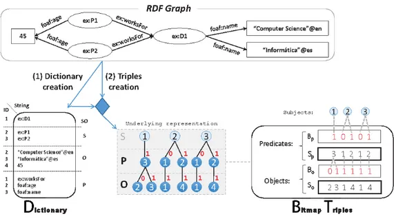
HDT encodes RDF into three components carefully described to address RDF peculiarities within a Publication-Interchange-Consumption workflow. The Header (H) holds the dataset metadata, including relevant information for discovering and parsing, hence serving as an entry point for consumption. The Dictionary (D) is a catalogue that encodes all the different terms used in the dataset and maps each of them to a unique identifier: ID. The Triples (T) component encodes the RDF graph as a graph of IDs, i.e. representing tuples of three IDs. Thus, Dictionary and Triples address the main goal of RDF compactness. Figure 2.8 shows how the Dictionary and Triples components are configured for a simple RDF graph. Each component is detailed below.

Dictionary. This component organizes the different terms in the graph according to their role in the dataset. Thus, four sections are considered: the section SO manages those terms playing both as subject and object, and maps them to the range[1, |SO|], being |SO| the number of different terms acting as subject and object. Sections S and O comprise terms that exclusively play subject and object roles respectively. Both sections are mapped from|SO|+1, ranging up to|SO|+|S| and|SO|+|O| respectively, where|S| and |O| are the number of exclusive subjects and objects. Finally, section P organizes all predicate terms, which are mapped to the range[1, |P|]. It is worth noting that no ambiguity is possible once we know the role played by the corresponding ID. Each section of the Dictionary is independently encoded to grasp its particular features. This allows important space savings to be achieved by considering that this sort of string dictionaries are highly compressible [86].

Triples. This component encodes the structure of the RDF graph after ID substitution. That is, RDF triples are encoded as groups of three IDs (ID-triples hereinafter): (ids idp ido), where

ids, idp, and ido are respectively the IDs of the corresponding subject, predicate, and object

terms in the Dictionary. The Triples component organizes all triples into a forest of trees, one per different subject: the subject is the root; the middle level comprises the ordered list of predicates

3

Figure 2.8: HDT Dictionary and Triples configuration for an RDF graph

reachable from the corresponding subject; and the leaves list the object IDs related to each (subject, predicate) pair. This underlying representation (illustrated in Figure 2.8) is effectively encoded following the BitmapTriples approach [36]. In brief, it comprises two sequences: Sp and So, concatenating respectively all predicate IDs in the middle level and all object IDs in the leaves; and two bitsequences:BpandBo, which are respectively aligned withSpandSo, using a 1-bit to mark the end of each list.

2.2.2 Building HDT

In this section we proceed to summarize how HDT is currently built4. Remind that this process is the main scalability bottleneck addressed by our current proposal.

To date, HDT serialization can be seen as a three-stage process:

• Classifying RDF terms. This first stage performs a triple-by-triple parsing (from the input dataset file) to classify each RDF term into the corresponding Dictionary section. To do so, it keeps a temporal data structure, consisting of three hash tables storing subject-to-ID, predicate-to-ID, and object-to-ID mappings. For each parsed triple, its subject, predicate, and object are searched in the appropriate hash, obtaining the associated ID if present. Terms not found are inserted and assigned an auto-incremental ID. These IDs are used to obtain the temporal ID-triples(ids idp ido)representation of each parsed triple, storing all them

in a temporary ID-triples array. At the end of the file parsing, subject and object hashes are processed to identify terms playing both roles. These are deleted from their original hash tables and inserted into a fourth hash comprising terms in the SO section.

• Building HDT Dictionary. Each dictionary section is now sorted lexicographically, because prefix-based encoding is a well-suited choice for compressing string dictionaries [85]. Finally, an auxiliary array coordinates the previous temporal ID and the definitive ID after the Dictionary sorting.

4

2.3. MAPREDUCE 19 • Building HDT Triples. This final stage scans the temporary array storing ID-triples. For each triple, its three IDs are replaced by their definitive IDs in the newly created Dictionary. Once updated, ID-triples are sorted by subject, predicate and object IDs to obtain the BitmapTriples streams. In practice, it is a straightforward task which scans the array to sequentially extract the predicates and objects into theSpandSosequences, and denoting list endings with 1-bits in the bitsequences.

2.2.3 Performance

HDT provides effective RDF decomposition, simple compression notions and basic indexed access in a compact serialization format which provides efficient access to the data. The Triples component is specifically encoded using a succinct data structure that enables indexed access to any triple in the dataset. It provides good performance both in terms of compression rate and query response time. With Plain-HDT Space savings of 12-16% are reported with real-world datasets5, although compression up to 7% is reached [36]. With HDT-Compress compression rates are improved to 2-4%, outperforming results of universal compressors by at least 20% [36]. Fernández et al. [36] compare Plain-HDT performance with state-of-the-art solutions such as RDF-3X and MonetDB. Tests are performed on the Dbpedia dataset with real-world queries. HDT outperforms both of them in all patterns except(?S,P,O), where RDF-3X obtains the best results, and(?S,P,?O), where HDT obtains the worst results.

2.2.4 Scalability Issues

HDT serialization process, described in section 2.2.2, makes use of several in-memory data structures: four hash tables to store term-to-ID mappings during the first stage, an auxiliary array during the second stage for temporary ID to definitive ID mappings, and an additional array to store ID-triples in the third phase. This is in addition to the actual Bitmap serialization, which must be wholly built in-memory before writing to disk.

2.3

MapReduce

MapReduce is a standard framework and programming model for the distributed processing of large amounts of data. Its main goal is to provide efficient parallelization while abstracting the complexities of distributed processing, such as data distribution, load balancing and fault tolerance [27]. MapReduce is not schema-dependent, so it can process unstructured and semi-structured data, although at the price of parsing every item [77]. A MapReduce job is comprised of two main phases:MapandReduce. The Map phase reads pairs key-value and ’maps’ relevant information, generating another intermediate pairs key-value. The Reduce phase takes all the values associated with the same key and ’reduces’ them into a smaller set of values [27].

MapReduce was originally developed by Google and published in 2004 [27]. Since then, it has been adopted by many companies that deal with Big Data. Examples of institutions actively contributing to the MapReduce ecosystem include:

• Google originally developed MapReduce [27] and many other related technologies: GFS [45] — an underlying file system to be used with MapReduce —, BigTable [20] — a distributed column-oriented database — , and Sawzall [99] — a procedural programming language for analysis of large datasets in MapReduce clusters.

5

• Apache developed Hadoop [10], a popular free implementation of MapReduce. Hadoop is continually under development and includes many other subprojects like HBase — a distributed columnar database inspired in BigTable — or Pig [95] — a procedural data language on top of Hadoop.

• Yahoo! has contributed to 80% of the core of Hadoop. In 2010 Hadoop clusters at Yahoo! spanned 25.000 servers, and stored 25 petabytes of application data, with the largest cluster being 3500 servers [108].

• Facebook devised Hive, an open-source data warehousing solution built on top of Hadoop [115]. In 2010 Facebook’s data warehouse that stored more than 15PB of data and loaded more than 60TB of new data every day [117].

• Microsoft created in 2008 their own approach to MapReduce: Cosmos, and SCOPE, a declarative language on top of Cosmos [19]. In recent years, Microsoft has abandoned its own technologies and has integrated Hadoop into their Cloud computing systems6 Although MapReduce is not dependent on filesystem architecture, its operation is based on distributed data across many nodes, in order to process chunks of data in the same node it is stored. Google File System (GFS) [45] and Hadoop Distributed File System (HDFS) are the main examples of those file systems. Google MapReduce and Hadoop are commonly deployed on top of them [27, 10].

2.3.1 Distributed FileSystems

To fully understand the MapReduce operation, it is needed to have some knowledge about the underlying distributed filesystem it operates on, which are portrayed in this section.

Distributed file systems serving data to MapReduce are designed to store and deliver large amounts of data on clusters of commodity hardware. They are designed to achieve scalability (i.e. scaling computation capacity by simply adding commodity servers) and high aggregate performance, while dealing with fault tolerance. To accomplish these goals these filesystems make use of physical architecture awareness, data replication and placement, constant monitoring, and instant recovery techniques [45, 13, 108].

Those filesystems are based on the premise of storing large quantities of data, which needs to be accessed sequentially by batch processes. Hence, some design principles are the basis of distributed filesystems [45].

• Data are stored on very large files: When working with high volume data sets, each one comprising GB or TB, and millions of objects, it is hard to manage billions of files. As a result, the file system stores the data as large files from hundreds of megabytes to terabytes. • High sustained bandwidth is more important than low latency: To data-intensive applications

a high rate of data transfer is more important that response time for each petition

• Data processing follows a “write once, read many times” pattern, with streaming file access: Once written, data are mostly accessed for data process, and is read often sequentially. Modification of files, whenever it happens, is usually by appending data. Random data modification is almost non-existent.

For these reasons, distributed filesystes are not suitable for all kinds of applications. Some operations are not efficient, such as the following [10]:

6

2.3. MAPREDUCE 21 • Low latency data access: Distributed file system are designed to deliver high-throughput

data-access. This is done at the expense of latency.

• Lots of small files: The complete namespace needs to be stored in-memory on a single node, which makes the storage of huge number of files unfeasible. This is in addition to under-usage of hard drives due to the block size used to store the files.

• Arbitrary file modifications: Modifications block files to the rest of the clients and require high usage of net bandwidth. Also, random modifications that do not affect end of files are not efficient.

2.3.1.1 Architecture

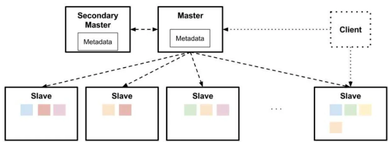
The architecture of distributed file systems are master/slave in nature. One master (Namenode in HDFS) contains metadata and file placement. Many slaves (chunkservers in GFS, datanodes in HDFS) store files data. Depending on the implementation, there can be “secondary masters” that maintain backups of the master or help with some operations. The general architecture is shown on Figure 2.9.

Figure 2.9: Distributed File System Architecture

Files are broken down in blocks and stored across the slaves. Block size is configurable, but is usually of at least 64 MB, and 128 MB are usually the norm nowadays [124]. This large size minimizes the cost of hard drive seeks, and reduces interaction with the master and metadata stored on it [45]. Some studies suggest that even larger sizes improve significantly the performance [77, 66]. Each block is replicated over a number of slaves. The replication factor is 3 by default, but is configurable. It is possible to configure different replication factor to specific files, if they are expected to be accessed more or less frequently than the average [45, 108]. If at any time replication of any block falls under its replication factor, it is copied to other nodes from active sources until it reaches the replication factor again.

Slaves and master communicate by heartbeats: Messages sent by each slave to the master periodically (3 seconds by default in Hadoop). If the master does not receive heartbeat from a slave in a specific timeframe (by default during 10 minutes in Hadoop) it is considered out of service and not used anymore. Heartbeats also carry information about total storage capacity, fraction of storage in use, and the number of data transfers currently in progress. These statistics are used for the master’s space allocation and load balancing decisions. The master sends maintenance commands to slaves in reply to heartbeats [108]

When a client needs to access a file, it send a petition to the master with file identification and offset. The master looks for the corresponding block and sends the client the list of slaves that store the block. The block is leased to the client for a specified period of time (60 seconds in GFS), although the client can request extensions. The client chooses a slave (typically the nearest one) and all the I/O operations are made through it. That avoids burdening the master with unnecessary data transfer. It is also possible for the client to ask for more than one block in a single request [45, 124, 108].

Multiple clients can read the same file with no additional features, but writings needs to deal with multiple clients trying to modify the same file. Different implementations take distinct approaches. HDFS only allows one client to write in the same file at a time [13, 108], GFS on the other allows multiple clients to append information to the same file. Data are stored in a temporary location in the nodes and is added to the file in the same order as the clients close the file [45].

In a write operation, slaves containing the block are sorted in a serial pipeline by proximity to the client, and one of them is chosen as the primary. The client writes data to the closest slave, and data are transferred through the pipeline. Receiving slaves send acknowledgment to the previous one. When all data has been transferred, primary client closes the file and wait for acknowledgment from other slaves. This acknowledgment contains a checksum that is validated. Master and client are informed of the end of the process and its final state [45, 108]. A write operation diagram is shown in Figure 2.10.

Figure 2.10: Distributed File System Write Dataflow

In the case of file creation, slaves are chosen according to a replica placement policy. This policy tries to achieve a compromise between transfer speed and fault tolerance. In HDFS, the default policy is to store the first replica in the same rack as the client, the second replica in another rack and the third replica in the same rack as the second one. If replication factor is greater than 3, following replicas are stored in random nodes over the cluster with this restrictions: No more than one replica is written on the same node, and no more than two replicas are written on the same rack [108].

2.3. MAPREDUCE 23 master and slave nodes; if not used during a specified time (3 days by default) they will by deleted by a background process [45, 13].

Load balancing must be taken into account when considering replica placement. GFS ponders current disk utilization rate of each node at write time [45]. HDFS, in contrast, does not consider it at write time in order to avoid placing new data into the same nodes. New data are frequently more accessed than older one, and placing most of it in a reduced number of slaves could affect performance. HDFS solution consist in running a load balancer as a background process; if a node exceeds a threshold, some of its block are moved to another slave in the cluster [124].

System metadata is stored in the namespace, which is stored by the in memory at runtime. It is periodically stored into disk as a checkpoint, but in order to make it efficiently, the master maintains a write-ahead commit log for changes to the namespace (journal on HDFS). The last checkpoint and the log are merged periodically to make changes persistent [45, 124].

Hadoop implements two other kind of nodes, which help the master in its duties. The Checkpoint Node reads checkpoint and journal, merges them into a single checkpoint, and returns it to the master. The Backup Node contains all metadata except block locations, reads the journal and creates its own checkpoints. If the master fails it can replace it [108].

GFS allows making snapshots by file or directory. When a snapshot is requested, the master revokes all leases, duplicates all the metadata referring to affected data, and points it to the same original blocks. When a client wants to modify a file, affected block are duplicated before any modification occurs [45]. HDFS only allows one snapshot and it can only be made at startup. A static checkpoint is written and slaves are notified to make local snapshots. When a slave needs to modify blocks, it makes a local copy before [108].

2.3.2 MapReduce

MapReduce is designed to abstract the complexities of distributed data process to designers. It aims to perform distributed computations over a high number of computers, dealing with issues like parallelization, data distribution, load balancing, fault tolerance and scalability in a transparent way [27].

In order to achieve these goals, MapReduce works with the principle of “moving algorithm to data”. That is, executing data process in the same nodes data are stored, rather than moving data over the machines that make the computations [27].

MapReduce model is based on two main operations, carried out in order: MapandReduce. These operations work with pairs value. Mappers input pairs and produces intermediate key-value pairs. An intermediate step groups all key-values with the same key, and Reducers read all grouped values with the same key and processes them, producing a smaller set of values [27]. A schema ofMapandReduceoperations can be seen in Figure 2.11

map: (k1, v1) →list(k2, v2)

reduce: (k2, list(v2)) →list(v2)

Figure 2.11: Map and Reduce input and output

MapReduce is I/O intensive, as it needs to write all intermediate data to disk between Map

andReducePhases. I/O is the main bottleneck in MapReduce performance. This also impacts in energy efficiency of MapReduce clusters. Many of current research lines try to deal with this problem [77].

2.3.2.1 Architecture

MapReduce clusters have a master/slave architecture. One master (Jobtracker in Hadoop) initial-izes the process, schedules tasks and keeps bookkeeping information. Many slaves (workers in Google MapReduce, Tasktrackers in Hadoop) executeMapandReducetasks [27]. A diagram of MapReduce architecture can be seen in Figure 2.12.

Figure 2.12: MapReduce Architecture Overview

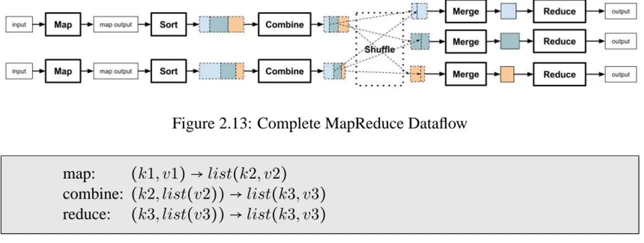
As stated before, a MapReduce job includes two main phases: Map andReduce, but more intermediate phases are needed in order to manage data. Below are presented all phases a MapReduce job, and is visually represented in Figure 2.13.

• Map: Reads input data and produces intermediate key/value pairs. • Sort: Map output is sorted by key.

• Combine (optional): Processes Map output in order to extract only meaningful data, its purpose is to minimize data transferred between Map and Reduce. If a Combine function is used, its usage is similar to Reduce, as seen in Figure 2.14.

• Shuffle: Data flows between Map and Reduce task. Data received by a Reduce task contains the same key.

• Merge: Data from different Map tasks is merged on the Reduce node.

• Reduce: Reads pairs key-value and produces a list of values. Each Reduce task works with only one key.

2.3. MAPREDUCE 25

Figure 2.13: Complete MapReduce Dataflow

map: (k1, v1) →list(k2, v2)

combine: (k2, list(v2)) →list(k3, v3)

reduce: (k3, list(v3)) →list(k3, v3)

Figure 2.14: Map, Combine and Reduce inputs and outputs

not possible withReducetask, as they need data generated by multiple Map tasks, each one ran in different nodes, so data transfer is unavoidable [124]. While both input and output are read from and written to distributed filesystems, this is not the case with intermediate values. They are temporary and replication would create unnecessary bandwidth usage [124].

When dividing input data into splits, it is important to take into account splits size. Smaller splits benefit load balancing, specially in heterogeneous environments, because they can be scheduled in different amount to each node. Bigger splits, by contrast, reduce the necessary overhead of scheduling and bookkeeping tasks [66]. The overhead is not only of processing time, but also of memory usage of the master node. This puts a de facto lower limit in split size. In addition, using split sizes bigger than block size of underlying distributed system is not recommended, as it could impact in data locality: If a split is bigger than a block, the probabilities of needing data transfer to retrieve part of the split are increased [27, 124].

MapReduce assigns nodes to different jobs using a scheduler. Usage of a FIFO scheduler is common in mono-user environments. In a FIFO scheduler all cluster nodes are used to process a MapReduce Job. When nodes are freed from a job, they can be used to process another job. This is the default scheduler in Hadoop, but in environments where more than one job is needed to run concurrently it is possible to use different schedulers. Hadoop allows to select a Fair Scheduler, that assign equal resources to each job, or a Capacity Scheduler, that uses a more complex scheduling with multiple queues, each of which is guaranteed to possess a certain capacity of the cluster [124, 77].

2.3.3 Challenges and Main Lines of Research

MapReduce is a young technology, with many challenges ahead and open lines of research. The most relevant are presented in this section.

2.3.3.1 Efficiency and Energy Issues

MapReduce is becoming a widespread solution for large-scale data analysis [78, 73]. With an architecture based in replication and constant data traffic and I/O operations, energy consumption is high [78]. This causes an energy waste that must be considered. Some studies that deal with this problem are:

• Covering Set: Keeps only a small fraction of the nodes powered up during periods of low usage. It can save between 9% and 50% of energy consumption [78].

• All-In Strategy: Uses all the nodes in the cluster to run a workload and then powers down the entire cluster. Presents lower effectiveness that Covering Set only when time needed to transition a node to and from a low power state is a relatively large fraction of the overall workload time. In all other cases the benefits of All-In Strategy are significant [73].

• Green HDFS: Proposes data-classification-driven data placement that allows scale-down by guaranteeing substantially long periods (several days) of idleness in a subset of servers in the datacenter. Simulation results show that GreenHDFS is capable of achieving 26% savings [68].

2.3.3.2 Complex Execution Paths

MapReduce reads a single input and produces a single output in a fixed execution path. Many execution plans require more complex path. There are solutions that implement the possibility to construct dataflow graphs with different possible paths [77]:

• Dryad: Execution engine that uses MapReduce but allows more general execution plans. A Dryad application combines computational “vertices” with communication “channels” to form a dataflow graph. Dryad runs the application by executing the vertices of this graph on a set of available computers, communicating as appropriate through files, TCP pipes, and shared-memory FIFOs [63]

2.3. MAPREDUCE 27

2.3.3.3 Declarative Languages

Developers working with MapReduce must code their own Map and Reduce procedures. If optimization is required, they could need to code Sort, Combine or Merge operations. Declarative languages have been developed to abstract queries from program logic. This allows query independence, reuse and optimization. Proposals of declarative languages include:

• Pig: Offers SQL-style high-level data manipulation constructs, which can be assembled in an explicit data flow and interleaved with custom Map- and Reduce-style functions or executables. Pig programs are compiled into sequences of Map-Reduce jobs, and executed in the Hadoop MapReduce environment. [95, 43].

• HiveQL: Queries are expressed in a SQL-like style, and are compiled into MapReduce jobs that are executed using Hadoop. In addition, HiveQL enables users to plug in custom MapReduce scripts into queries. [115, 116].

• SCOPE: Designed for ease of use with no explicit parallelism, while being amenable to efficient parallel execution on large clusters. SCOPE borrows several features from SQL. Data are modeled as sets of rows composed of typed columns. The select statement is retained with inner joins, outer joins, and aggregation allowed. Users can easily define their own functions and implement their own versions of operators: extractors (parsing and constructing rows from a file), processors (row-wise processing), reducers (group-wise processing), and combiners (combining rows from two inputs). SCOPE supports nesting of expressions but also allows a computation to be specified as a series of steps [19].

• DryadLINQ: A DryadLINQ program is a sequential program composed of LINQ expres-sions performing arbitrary side-effect-free operations on datasets, and can be written and debugged using standard .NET development tools. The DryadLINQ system automatically and transparently translates the data-parallel portions of the program into a distributed exe-cution plan which is passed to the Dryad exeexe-cution platform [62].

2.3.3.4 Progress Estimation

Hadoop speculative task scheduling compares node progress with the average. This approach can present problems when applied over heterogeneous hardware, in which progress rate can vary from one node to another [77]. Solutions to deal with this issue include:

• Longest Approximate Time to End (LATE): Proposes estimating task finalization through individual progress rate. Improves Hadoop response times by a factor of 2 in heterogeneous cluster environments [128].

• Parallax: Targets environments where queries consist of a sequential paths of MapReduce jobs and is fully implemented in Pig. It handles varying processing speeds and degrees of parallelism during query execution [91]

• ParaTimer: Estimates the progress of queries that translate into directed acyclic graphs of MapReduce jobs, where jobs on different paths can execute concurrently. The essential techniques involve identifying the critical path for the entire query and producing multiple time estimates for different assumptions about future dynamic conditions. [90]