MPC Bases energy mangement system for hybrid renewable energies

Texto completo

(1)UNIVERSITY OF VALLADOLID School of Industrial Engineering Department of Systems Engineering and Automation. DOCTORAL THESIS MPC-BASED ENERGY MANAGEMENT SYSTEM FOR HYBRID RENEWABLE ENERGIES by Johanna Carolina Salazar Salas. Supervisors: Dr. Fernando Tadeo Dr. Cesar de Prada. Thesis submitted to the University of Valladolid in partial fulfillment of the requirements for the doctoral degree.. September 2015.

(2)

(3) Acknowledgements La presente tesis doctoral no es más que la suma de la paciencia, dedicación y colaboración de un gran número de personas. Por lo que tratar de enumerar en una página sus nombres resulta difícil si se considera la poca disponibilidad de papel que tenemos para dar con justicia todos los créditos y méritos a quienes se los merecen. Por tanto, quiero agradecerles a todos ellos cuanto han hecho por mí, para que este trabajo saliera adelante de la mejor manera posible. Primeramente deseo agradecer a mis padres, mi abuela y mi hermano por su apoyo y comprensión, sin los cuales no hubiera podido realizar esta tesis doctoral. En especial agradezco a mi madre por animarme a dar mis primeros pasos en la investigación. Mi definición no es más que aquello que moldearon en mi infancia. A Reyes, José, Laura y Diego por abrirme las puertas de su hogar. Agradezco los ánimos que me daban cada día para seguir en mi investigación. A mis supervisores Fernando Tadeo y Cesar de Prada por aceptar la realización de esta tesis doctoral bajo su dirección, por su confianza en mi trabajo, por haberme facilitado siempre los medios suficientes para llevar a cabo todas las actividades propuestas durante el desarrollo de esta tesis, por solventar todas mis dudas referentes al campo de la automática, por su capacidad en guiar mis ideas y prestarme las suyas. Agradezco a todos mis compañeros y amigos del Departamento de Ingeniería de Sistemas y Automática en la Universidad de Valladolid y del CTA con los cuales he compartido despacho e incontables horas de trabajo: Alvaro Serna, Daniel Navia, Diego Napp, Elena Gomez, Imene Yahyaoui, Ines Zaidi, Luis Palacin, María Pereda, Meriem Nachidi, Mohamed Bolajraf y Ruben Martí. En especial a Miguel Rodríguez y Daniel Sarabia por su disponibilidad y paciencia que hizo que nuestras discusiones redundaran benéficamente tanto a nivel científico como personal. También me complace reconocer la acogida, el apoyo y los medios recibidos en los distintos centros donde he desarrollado parte de mi Doctorado: el Proyecto Open Gain, el Departamento de Ingeniería de Electrónica y Computación en la Universidad de Limerick, el Departamento de Lenguajes y Computación en la.

(4) Universidad de Almería, la Plataforma Solar de Almeria; y el Departamento de Ingeniería de Sistemas y Automática en la Universidad de Sevilla. Agradezco a todos mis compañeros y amigos del Proyecto Open Gain: Kamilia Ben Youssef y Sami Karaki, del Departamento de Ingeniería de Electrónica y Computación en la Universidad de Limerick: Martin Hayes, Kritchai Witheephanich, Anthony Fee y Juan Manual Escaño; del Departamento de Lenguajes y Computación en la Universidad de Almería: Manuel Pasamontes, Francisco Rodríguez, José Domingo Álvarez, María del Mar Castilla, Sabrina Rosiek, Helton Scherer y Ricardo Silva; de la Plataforma Solar de Almeria: Lidia Roca; del Departamento de Ingeniería de Sistemas y Automática en la Universidad de Sevilla: Carlos Bordons y Luis Valverde. A las siguientes instituciones que contribuyeron a financiar este trabajo:  Ministerio de Educación y Ciencia, programa de becas de formación del profesorado universitario (FPU) referencia Nº AP2008-03557.  Proyecto Singular Estratégico sobre Arquitectura Bio-Climática y Frío Solar, PSE_Arfrisol PS-120000-2005-1.  Beca de Estancia Breve de la Universidad de Valladolid. Finalmente, y por encima de todo, tengo que agradecer a Pablo por apoyarme cada día. A él le debo parte de esta tesis, y aunque no pueda incluir su nombre como autor, sinceramente debo confesar su participación..

(5) Abstract Environmental pollution and the gradual depletion of conventional energy have induced significant research in energy supply systems equipped with renewable and conventional sources. Although wind and solar energy sources emerge as the most promising renewable energies, a supply system comprising two or more sources is recommended to fulfill local loads, as the power generated by renewable sources depends on weather conditions. For this, storage devices are frequently used to store the excess energy generated by the renewable sources and conventional energy sources are used as backup when the production of renewable energies is low and the energy stored is not enough to fulfill the load. The main idea of any energy supply system is to fulfill the energy demand with the minimum cost, considering the operational constraints related to the components. As a result, some issues, such as security of supply, improvement in the combination of energy sources, efficiency, energy saving, improvement in access to isolated systems, and the development of renewable energy, should all be taken into account. Up to now, cost reduction and energy saving have been understood almost exclusively as the technological improvement of renewable sources: wind turbines, solar panels, solar collectors, etc. The misconception of “the best system is made with the best components” is still used for the design of energy supply systems. An optimum system is typically more complex than the sum of the components which integrate the system. Technological advances in renewable sources should be coupled with a sophisticated energy management system. This thesis proposes an energy management system based on control ideas. From a control point of view, the main difficulty is their dynamics, defined according to differential equations and logic rules. Therefore, in this thesis, the design of a hybrid controller based on predictions of energy, estimated from physical models and previous measurements, is considered in order to satisfy the energy supply. Model Predictive Control (MPC) has been chosen as the main control strategy since it is able to handle variations in the supply of renewable energy; while, in the energy demand, MPC includes a cost function to be minimized and adds the.

(6) 6. Abstract. constraints on the manipulated and controlled variables. The cost function takes into account the value of the energy generated, the cost of storing energy locally, and the aging of the components. A process model that represents the process dynamic is used to predict the output signal accurately. It is selected to be simple because the future control actions computed by the optimizer take into account the integration of the model along the prediction horizon. Hybrid process models are then considered in the proposed MPC. Although this gives formulation problems, Mixed Logical Dynamic (MLD) involves continuous variables (involved in linear dynamic equations), discrete variables (specified through propositional logic statements), and the mutual interaction between the two. In this case, the resulting mixed integer quadratic programming (MIQP) could present problems for real time implementation, because the solution is computationally complex and depends exponentially on the number of binary manipulated variables. To simplify the MPC problem, the use of binary manipulated variables is avoided by the parameterization of the binary manipulated variables into continuous variables. This transforms the mixed integer optimization into a nonlinear optimization made up of only by continuous manipulated variables (NMPC). To illustrate the applicability and effectiveness of the proposed predictive control, four energy supply systems have been considered: a Solar and Wind based Microgrid for Desalination, a Solar Gas Air Conditioning Plant, a Hydrogen based Microgrid, and a Solar Desalination Plant. The study and applicability of these energy supply systems will be carried out throughout the different chapters. The proposed algorithms are demonstrated in detail using simulations of existing systems, and are partially validated in these systems. The implementation has been done as a modular structure to facilitate changes. Additionally, a library on microsources of renewable energies has been developed in EcosimPro©, as it is a powerful modeling and simulation tool that follows an advanced methodology for modeling and dynamic simulation. The renewable energy library facilitates the training of technicians and engineers in how to operate energy supply systems, how to check different configurations and control strategies, before implementing them, and how to facilitate their design..

(7) Contents Chapter 1 Introduction .............................................................................................. 21 1.1.- Objective..................................................................................................... 22 1.1.1.- Electrical energy supply system ....................................................... 25 1.1.2.- Thermal energy supply system ......................................................... 26 1.2.- Model Predictive Control (MPC) ............................................................... 28 1.3.- Nonlinear Predictive Control ...................................................................... 32 1.4.- Outline of the Chapter ................................................................................ 34 1.5.- Summary of Publications ............................................................................ 35 Chapter 2. Wind Turbine Control ........................................................................... 39. 2.1.- Process Description .................................................................................... 39 2.2.- Wind Turbine Model .................................................................................. 43 2.2.1.- Aerodynamic Model ......................................................................... 43 2.2.2.- Hydraulic Actuator Model ............................................................... 44 2.2.3.- Drive Train Model............................................................................ 45 2.2.4.- Permanent Magnet Synchronous Generator Model .......................... 45 2.3.- Simulations Platform .................................................................................. 49 2.4.- Traditional Wind Turbine Control .............................................................. 50 2.4.1.- Linearized Wind Turbine Model ...................................................... 55 2.5.- Simulation Results for Traditional Control ................................................. 57 2.6.- Nonlinear Predictive Control ...................................................................... 59 2.7.- Simulations Results for NMPC................................................................... 60 2.8.- Conclusions ................................................................................................ 62 Chapter 3 Solar and Wind Based Microgrid for Desalination .................................. 63 3.1.- Process Description .................................................................................... 64.

(8) 8. Contents. 3.2.- Renewable Energy Source Model .............................................................. 69 3.2.1.- Wind Turbine ................................................................................... 70 3.2.2.- Solar Panels Model .......................................................................... 72 3.2.3.- Battery Bank Model ......................................................................... 79 3.2.4.- Diesel Generator Model ................................................................... 82 3.3.- Microgrid Operation Model ....................................................................... 82 3.3.1.- Current Source Inverter Model (CSI) .............................................. 85 3.3.2.- Voltage Source Inverter Model (VSI) .............................................. 86 3.4.- Reverse Osmosis Desalination Model ........................................................ 89 3.5.- Simulation Platform ................................................................................... 94 3.6.- Renewable Ecosimpro Library ................................................................... 95 3.7.- Disturbance Prediction Models .................................................................. 97 3.7.1.- Water Demand Prediction Model .................................................... 97 3.7.2.- Wind Speed Prediction Model ......................................................... 98 3.8.- Hybrid Systems .......................................................................................... 98 3.8.1.- Model Predictive Control for Hybrid Systems ................................. 99 3.8.2.- Predictive and Control Horizon ..................................................... 101 3.8.3.- Mathematical Formulation ............................................................. 102 3.9.- Hybrid Model Predictive Control ............................................................. 104 3.10.- Simulation Results .................................................................................. 107 3.11.- Conclusions ............................................................................................ 110 Chapter 4 Solar/Gas Climatization Plant ................................................................ 111 4.1.- Process Description .................................................................................. 111 4.2.- Solar Air Conditioning Model .................................................................. 116 4.2.1.- Solar Collector Model .................................................................... 117 4.2.2.- Gas Heater Model .......................................................................... 120 4.2.3.- Storage Tanks Model ..................................................................... 123 4.2.4.- Absorption Machine Model ........................................................... 127 4.2.5.- Flow Model .................................................................................... 131 4.2.6.- Power Pump Model........................................................................ 133.

(9) Contents. 9. 4.3.- Simulation Platform .................................................................................. 134 4.4.- Disturbance Prediction Model .................................................................. 135 4.4.1.- Irradiation Prediction Model .......................................................... 136 4.4.2.- Ambient Temperature Prediction Model ........................................ 137 4.5.- Hybrid Model Predictive Control ............................................................. 137 4.6.- Validation ................................................................................................. 141 4.6.1.- Validation by simulation ................................................................ 141 4.6.2.- Experimental validation ................................................................. 144 4.7.- Hybrid Model Predictive Control Platform .............................................. 146 4.8.- Conclusions .............................................................................................. 148 Chapter 5 Hydrogen Based Microgrid .................................................................... 149 5.1.- Process Description .................................................................................. 150 5.2.- Hydrogen-Based Microgrid Model ........................................................... 152 5.2.1.- Hydrogen Energy Storage .............................................................. 152 5.2.2.- Solar Panels Model ........................................................................ 156 5.2.3.- Battery Bank Model ....................................................................... 158 5.3.- Case Study ................................................................................................ 160 5.3.1.- Electrolyzer .................................................................................... 160 5.3.2.- Fuel Cell ......................................................................................... 161 5.4.- Hybrid Model Predictive Control ............................................................. 161 5.4.1.- Cost function .................................................................................. 161 5.4.2.- Constraints ..................................................................................... 162 5.4.3.- Transformation into a solvable optimization .................................. 164 5.5.- Simulation Results .................................................................................... 167 5.6.- Conclusions .............................................................................................. 170 Appendix A Renewable Energy Library ................................................................ 171 A.1.- General Component ................................................................................. 171 A.2.-Ports .......................................................................................................... 172 A.3.-Componets Description............................................................................. 173 A.3.1.- Wind Turbine Component ............................................................ 174.

(10) Contents. 10. A.3.2.- Wind Controller Component ......................................................... 175 A.3.3.- Solar Panels Component ............................................................... 176 A.3.4.- Solar Control Component. ....................................... 177. A.3.5.- Battery Bank Component .............................................................. 178 A.3.6.- Diesel Generator Component ........................................................ 179 A.3.7.- Diesel Generator Controller Component ....................................... 180 A.3.8.- Microgrid Component ................................................................... 181 A.3.9.- Microgrid Control Component ...................................................... 182 A.3.10.- Desalination Component ............................................................. 184 A.3.11.- Water Demand Component ......................................................... 185 A.3.12.- Solar Irradiation Component ....................................................... 185 A.3.13.- Ambient Temperature Component .............................................. 186 Appendix B Diesel Generaton .............................................................................. 189 B.1.- Model of Diesel Engine System .............................................................. 189 B.1.1.-Current Driver Model ..................................................................... 190 B.1.2.-Actuator Model .............................................................................. 190 B.1.3.-Diesel Engine Model ...................................................................... 190 B.1.4.-Flywheel Model ............................................................................. 192 B.2.-Synchronous Generator Model ................................................................. 192 B.3.-Excitation System Model .......................................................................... 193 B.3.1.-Self-Excited DC Exciter ................................................................. 195 B.4.-Speed Control ........................................................................................... 196 B.5.-Automatic Voltage Regulation ................................................................. 196.

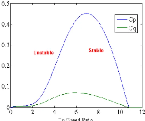
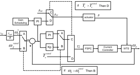
(11) List of Figures Figure 1.1.- Solar, Wind and battery based Microgrid ............................................. 23 Figure 1.2.- Solar and Hydrogen - based Microgrid ................................................. 23 Figure 1.3.- Solar Gas Air Conditioning Plant ......................................................... 24 Figure 1.4.- MPC Strategy........................................................................................ 29 Figure 1.5.- MPC Strategy........................................................................................ 30 Figure 2.1.- Wind Turbine Components ................................................................... 40 Figure 2.2.- Wind Turbine components into nacelle ................................................ 40 Figure 2.3.- Wind Turbine Model ............................................................................ 41 Figure 2.4.- Operation Region of Wind Turbine ...................................................... 42 Figure 2.5.- Power Coefficient vs. Tip-Speed Ratio................................................. 42 Figure 2.6.- Operational Constraints of a variable speed Wind Turbine .................. 43 Figure 2.7.- Power Coefficient vs. Tip-Speed Ratio................................................. 44 Figure 2.8.- Hydraulic Actuator Model .................................................................... 45 Figure 2.9.- Current Controller Model ..................................................................... 47 Figure 2.10.- Decoupling between |d| and |q| axis ................................................... 47 Figure 2.11.- Current controller scheme considering |d| and |q| axis ....................... 48 Figure 2.12.- Simulink boxes of the Wind Turbine ................................................. 49 Figure 2.13.- Operational regions of Wind Turbines ............................................... 51 Figure 2.14.- Control scheme in Middle Wind Speed ............................................. 51 Figure 2.15.- Unstable and stable regions over Cp-λ and Cq-λ curve ..................... 52 Figure 2.16.- Control scheme in High Wind Speed ................................................. 53 Figure 2.17.- Lineal interpolation of the pitch controller gains ............................... 53 Figure 2.18.- Operating points proper of zone III .................................................... 54 Figure 2.19.- Overview of the whole control scheme .............................................. 54.

(12) 12. List of Figures. Figure 2.20.- System Response considering traditional PID control ....................... 58 Figure 2.21.- Nonlinear Predictive Control scheme ................................................ 59 Figure 2.22.- System Response considering Nonlinear Predictive Control ............. 61 Figure 3.1.- Microgrid for desalination in remote areas ........................................... 64 Figure 3.2.- Mixed DC and AC coupled concept ..................................................... 65 Figure 3.3.- Pure AC coupled concept ..................................................................... 66 Figure 3.4.- Prototype built at Borj Cedria by Open-Gain Workgroup .................... 66 Figure 3.5.- Control strategy proposed by Open Gain workgroup [63]. .................. 67 Figure 3.6.- Wind and solar based microgrid used in this thesis .............................. 68 Figure 3.7.- Wind Turbine control diagram ............................................................. 70 Figure 3.8.- Operating Regions of Wind Turbine .................................................... 71 Figure 3.9.- Photovoltaic Panels control diagram .................................................... 73 Figure 3.10.- Circuit diagram of a solar cell ............................................................ 73 Figure 3.11.- I-V and P-V photovoltaic array characteristic ................................... 78 Figure 3.12.- Irradiation influence on PV array characteristics I-V curves ............. 78 Figure 3.13.- Irradiation influence on PV array characteristics P-V curves ............ 78 Figure 3.14.- Temperature influence on PV array characteristics I-V curves ......... 79 Figure 3.15.- Temperature influence on PV array characteristics P-V curves......... 79 Figure 3.16.- Circuit diagram of a battery ............................................................... 80 Figure 3.17.- The overall block diagram of diesel generator ................................... 82 Figure 3.18.- Droop Mode: Active Power/Frequency-relation ................................ 84 Figure 3.19.- Droop Mode: Reactive Power/Voltage-relation................................. 84 Figure 3.20.- Current Source Inverter Control ........................................................ 85 Figure 3.21.- Local Secondary Load-Frequency Control ........................................ 86 Figure 3.22.- Voltage Source Inverter Control ........................................................ 87 Figure 3.23.- Control approach selfsync by ISET (Engler, [81]) ............................. 87 Figure 3.24.- Three phase selfsync control algorithm .............................................. 88 Figure 3.25.- Direct and Reverse Osmosis Process ................................................. 89 Figure 3.26.- Reverse Osmosis Plant....................................................................... 90 Figure 3.27.- Desalination Plant Model ................................................................... 90.

(13) List of Figures. 13. Figure 3.28.- Pump performance curves .................................................................. 91 Figure 3.29.- Stratified modeling of the RO membranes ......................................... 93 Figure 3.30.- Experimental results for a constant load of 3kW per line .................. 95 Figure 3.31.- Some elements for Renewable Energy Library .................................. 96 Figure 3.32.- Binary Variable parameterization ui................................................. 100 Figure 3.33.- Nonlinear Predictive Control Implementation ................................. 101 Figure 3.34.- Prediction and Control Horizon ....................................................... 102 Figure 3.35.- Prediction and Control Horizons of the variables δgen and δfeed ........ 106 Figure 3.36.- Parameterization of the desalination flow qdes.................................. 107 Figure 3.37.- Hybrid controller over solar/wind-based microgrid ......................... 110 Figure 4.1.- Scheme of the Solar Heat Supply System ........................................... 112 Figure 4.2.- Solar/gas heat supply system prototype built at Almeria .................... 113 Figure 4.3.- Continuous valves configuration of the storage tanks ........................ 114 Figure 4.4.- Scheme of the solar collector subsystem ............................................ 117 Figure 4.5.- Schematic for parameter estimation .................................................... 118 Figure 4.6.- Inputs values for solar collector validation ......................................... 119 Figure 4.7.- Validation of solar collector model ..................................................... 120 Figure 4.8.- Scheme of the gas heater subsystem ................................................... 120 Figure 4.9.- Power supplied by the burning gas ..................................................... 121 Figure 4.10.- Schematic for parameter estimation ................................................. 121 Figure 4.11.- Inputs values for Gas Heater (ON Mode) ........................................ 122 Figure 4.12.- Inputs values for Gas Heater (OFF Mode) ....................................... 122 Figure 4.13.- Validation of Gas Heater (ON Mode) .............................................. 123 Figure 4.14.- Validation of Gas Heater (OFF Mode) ............................................ 123 Figure 4.15.- Scheme of the accumulation subsystem ........................................... 124 Figure 4.16.- Schematic for parameter estimation ................................................. 125 Figure 4.17.- Validation of Storage Tanks Model ................................................. 127 Figure 4.18.- Scheme of the Absorption Machine ................................................. 128 Figure 4.19.- Scheme of the absorption machine ................................................... 129 Figure 4.20.- Heat absorbed by the generator of the absorption machine.............. 130.

(14) 14. List of Figures. Figure 4.21.- Schematic for parameter estimation ................................................. 130 Figure 4.22.- Validation of the Generator Circuit Model ...................................... 131 Figure 4.23.- Scheme of the Solar Heat Supply System ........................................ 131 Figure 4.24.- Schematic for parameter estimation of flow model ......................... 132 Figure 4.25.- Model for q1 ..................................................................................... 132 Figure 4.26.- Model pump nonlinearities for q6 .................................................... 132 Figure 4.27.- Power pump performance curve ...................................................... 133 Figure 4.28.- Schematic for parameter estimation ................................................. 134 Figure 4.29.- Validation of the Power Pump Model.............................................. 134 Figure 4.30.- Solar Gas Air Conditioning Platform............................................... 135 Figure 4.31.- Validation of the Irradiation Prediction Model ................................ 136 Figure 4.32.- Validation of the Ambient Temperature Prediction Model ............. 137 Figure 4.33.- Structure of the prediction and control horizons .............................. 140 Figure 4.34.- Implementation of the Nonlinear Controller .................................... 141 Figure 4.35.- Working point of the pump PB01 ...................................................... 141 Figure 4.36.- Power consumed by the pump PB01.................................................. 142 Figure 4.37.- Water temperature from solar collector field ................................... 142 Figure 4.38.- Temperature of stored water in the tanks ......................................... 142 Figure 4.39.- Connection/Disconnection of gas heater .......................................... 142 Figure 4.40.- Thermal Energy produced by gas heater. ......................................... 143 Figure 4.41.- Water temperature at the inlet of the absorption machine. .............. 143 Figure 4.42.- Working point of the pump PB01 ...................................................... 144 Figure 4.43.- Power consumed by the pump PB01.................................................. 144 Figure 4.44.- Water temperature from solar collector field ................................... 144 Figure 4.45.- Temperature of stored water in the tanks ......................................... 145 Figure 4.46.- Connection/Disconnection of gas heater .......................................... 145 Figure 4.47.- Thermal energy produced by gas heater .......................................... 145 Figure 4.48.- Water temperature at the inlet of the absorption machine ............... 145 Figure 4.49.- OPC Exchange Data Diagram ......................................................... 146 Figure 4.50.- Solar Gas Air Conditioning OPC Configuration ............................. 147.

(15) List of Figures. 15. Figure 5.1.- A hydrogen-based microgrid system .................................................. 151 Figure 5.2.- A hydrogen energy storage Diagram .................................................. 153 Figure 5.3.- Polarization curve of losses ................................................................ 154 Figure 5.4.- Photovoltaic Panel control diagram .................................................... 156 Figure 5.5.- Equivalent circuit of a solar cell ......................................................... 157 Figure 5.6.- Equivalent circuit of a battery ............................................................. 158 Figure 5.7.- V-I characteristic curve of PEM electrolyzer at 26ºC ......................... 160 Figure 5.8.- V-I characteristic curve of PEM fuel cell ........................................... 161 Figure 5.9.- Structure of the variables δfc and δez during the Prediction and Control Horizons .............................................................................................. 164 Figure 5.10.- Parameterization of the grid power Pgrid .......................................... 165 Figure 5.11.- Parameterization of the fuel cell power Pfc ...................................... 166 Figure 5.12.- Implementation of the Nonlinear Controller .................................... 166 Figure 5.13.- Solar Radiation ................................................................................. 168 Figure 5.14.- Ambient Temperature ...................................................................... 168 Figure 5.15.- Power consumed by the load ............................................................ 168 Figure 5.16.- Power produced by the solar panels ................................................. 168 Figure 5.17.- Power delivered by the fuel cell ....................................................... 168 Figure 5.18.- Power consumed by the electrolyzer ................................................ 168 Figure 5.19.- Power generated or consumed by the main grid .............................. 169 Figure 5.20.- Power delivered or consumed by the battery bank ........................... 169 Figure 5.21.- Current of the battery bank .............................................................. 169 Figure 5.22.- State of charge of the battery bank ................................................... 169 Figure 5.23.- Metal hybrid level ............................................................................ 169 Figure A.1.- Symbol of WindTurbineModel Component ..................................... 174 Figure A.2.- Symbol of the Component ControlTurbine...................................... 176 Figure A.3.- Symbol of SolarPanelsModel Component ....................................... 176 Figure A.4.- Symbol of the Component ControlSolar ......................................... 177 Figure A.5.- Symbol of BatteryBank Component ................................................ 178 Figure A.6.- Symbol of DieselGenerator Component .......................................... 180.

(16) 16. List of Figures. Figure A.7.- Symbol of ControlGenerator Component ....................................... 180 Figure A.8.- Symbol of InversorSolar Component .............................................. 181 Figure A.9.- Symbol of InversorWind Component .............................................. 181 Figure A.10.- Symbol of InversorBattery Component ........................................... 182 Figure A.11.- Symbol of InversorBattery Component ........................................... 183 Figure A.12.- Symbol of SecondFreqCtrl Component .......................................... 183 Figure A.13.- Symbol of DesalinationPlant Component ....................................... 184 Figure A.14.- Symbol of ForecastWater Component ............................................ 185 Figure A.15.- Symbol of ForecastSolar Component ............................................. 186 Figure A.16.- Symbol of ForecastTemperature Component ................................. 186 Figure B.1.- The overall block diagram of diesel generator ................................. 189 Figure B.2.- Block diagram of a typical diesel engine system ............................. 190 Figure B.3.- Typical variation of dead time with engine speed ........................... 191 Figure B.4.- Funtional Block diagram of a synchronous generator excitation control system (Kundur, [139]) .......................................................... 194 Figure B.5.- Block Diagram of a self- excited DC exciter ................................... 195.

(17) List of Tables Table 2.1.- Parameters for mechanical model of the WTs ...................................... 50 Table 2.2.- Parameters for electrical model of the WTs .......................................... 50 Table 3.1.- Solar Panel Parameters ......................................................................... 77 Table 3.2.- Battery Bank Parameters....................................................................... 82 Table 4.1.- Variables for solar collector model ..................................................... 118 Table 4.2.- Parameters for solar collector model .................................................. 118 Table A.1.- Controlled Variables belong to Controlled Port.................................. 173 Table A.2.- Manipulated Variables belong to Manipulated Port ........................... 173 Table A.3.- Disturbance Variables belong to Disturbance Port ............................. 173 Table A.4.- Wind Turbine Component Attributes ................................................. 174 Table A.5.- Ports associated to WindTurbineModel Component .......................... 175 Table A.6.- Wind Turbine Control Component Attributes .................................... 175 Table A.7.- Ports associated to ControlTurbine Component ................................. 176 Table A.8.- Solar Panels Component Attributes .................................................... 177 Table A.9.- Ports associated to WindTurbineModel Component .......................... 177 Table A.10.- Solar Panels Control Component Attributes .................................... 178 Table A.11.- Ports associated to ControlSolar Component ................................... 178 Table A.12.- Batteries Bank Component Attributes .............................................. 179 Table A.13.- Ports associated to BatteryBank Component ................................... 179 Table A.14.- DieselGenerator Component Attributes ........................................... 180 Table A.15.- Ports associated to DieselGenerator Component ............................. 180 Table A.16.- ControlGenerator Component Attributes ......................................... 180 Table A.17.- Ports associated to ControlGenerator Component ........................... 181 Table A.18.- InversorSolar Component Attributes ............................................... 181.

(18) 18. List of Tables. Table A.19.- Ports associated to InversorSolar Component ................................. 181 Table A.20.- InversorWind Component Attributes ............................................... 182 Table A.21.- Ports associated to InversorWind Component ................................. 182 Table A.22.- InversorBattery Component Attributes ............................................ 182 Table A.23.- Ports associated to InversorBattery Component .............................. 182 Table A.24.- BatteryCtrl Component Attributes ................................................... 183 Table A.25.- Ports associated to BatteryCtrl Component ..................................... 183 Table A.26.- SecondFreqCtrl Component Attributes ............................................ 184 Table A.27.- Ports associated to SecondFreqCtrl Component .............................. 184 Table A.28.- DesalinationPlant Component Attributes......................................... 185 Table A.29.- Ports associated to DesalinationPlant .............................................. 185 Table A.30.- ForecastWater Component Attributes .............................................. 185 Table A.31.- Ports associated to ForecastWater Component ................................ 185 Table A.32.- ForecastSolar Component Attributes ............................................... 186 Table A.33.- Ports associated to ForecastSolar Component ................................. 186 Table A.34.- ForecastTemperature Component Attributes ................................... 186 Table A.35.- Ports associated to ForecastTemperature Component ..................... 187.

(19) Glossary ARX CARIMA CIESOL CSI DER DMC DTC-GPC EPSAC FSP GPC IDCOM IMC MIPC MHL MPC MPPT NLP NMPC NOCP NOCT OPC OPEN-GAIN. PEM PFC PI PMSG PV PWM. AutoRegressive Model with eXternal input Controlled AutoRegressive Integrated Moving Average Centro Mixto de Investigación de la Energía SOLar. Current Source Inverter Distributed Energy Resource Dynamic Matrix Control Dead-Time Compensator Generalized Predictive Controller Extended Prediction Self Adaptive Control Filtered Smith Predictor Generalized Predictive Control Model Predictive Heuristic Control Internal Model Control Mixed Integer Predictive Control Metal Hybrid Level Model Predictive Control. Maximum Power Point Tracking Nonlinear Programming Nonlinear Model Predictive Control Nonlinear Optimal Control Problem Nominal Operation Cell Temperature Open Process Control Open Process Control Optimal Engineering Design for Dependable Water and Power Generation in Remote Areas using renewable energies and Intelligent Automation Proton Exchange Membrane Predictive Functional Control. Proportional Integral controller Permanent Magnet Synchronous Generator Photovoltaic Panels. Pulse Width Modelation.

(20) Glossary. 20. RO SCADA SQP STC SVM VSI WTs. Reverse Osmosis Supervisory Control And Data Acquisition Sequential Quadratic Programming Standard Test Conditions Space-Vector Modulation. Voltage Source Inverter Wind Turbine System.

(21) CHAPTER 1. Introduction The standard of living is being affected by a variety of far-reaching changes: technological development, globalization, accelerated innovation, new economic order, etc. If the industrial revolution was characterized by significant changes in the production systems and the 20th century was identified by mobility and communications, the coming years will be defined by the development of new technologies and their application to different fields. Two different visions are present in the interaction between new technologies and the environment: one holds that nature will be destroyed if the interaction between humans and the environment does not change, and it points out that the current development model will lead to the destruction of the environment and, as a consequence, of humanity; the other defends the need of the current model for economic development as a condition of human evolution and believes that if the current model is stopped, it would be the end of the current civilization. A third point of view arises within this situation of change, where people begin to be aware that scientific knowledge has improved the quality of life through material progress, but that, at the same time, it has brought serious problems related to the environment. In order to avoid this, economic development aims to be compatible with the protection of the environment in what is called sustainable development. Notice that the energy topic plays an important role within sustainable development. The accelerated development of industrialized societies has been possible due to an intensive use of fossil fuels, which has led to an increase in environmental pollution and the development of dangerous phenomena such as global warming, acid rain, desertification, freshwater pollution or ozone fluctuation, all of which can cause serious damage to humans. For this reason, the world should base its policies on satisfying the energy demand with minimum cost, where conditions are able to ensure the supply and environmental protection. As a result, some issues, such as security of supply, improvement in the combination of energy sources, efficiency,.

(22) 22. Chapter 1. Introduction. energy savings, improvement in access to isolated systems and the development of renewable energy, will all be considered in the coming years. To sum up, a more effective use of fossil fuels and the search for a variety of energy sources is required to avoid dependency on the producing countries, damage to the environment and a quick depletion of fossil fuels. For this, renewable energies are being considered with great interest, looking to increase their efficiency and make them competitive with conventional systems. Wind and solar sources are two of the most promising renewable power generation technologies. As the power generated by renewable energy sources depends on weather conditions when using them, it is recommended to combine some different renewable sources in the system. Additionally, the extra energy generated by the renewable sources should be stored in storage devices to cover the time periods of low power production by renewable sources. An energy supply system comprising some renewable and conventional sources, together with a high level of automation, have caught the attention of research worldwide as it has a great potential to provide higher quality and more reliable power to customers than a system based on a single resource. These systems take advantage of the mutual complementarities between sources so that the capacity of the storage device is greatly reduced, while the economic performance and operating reliability of the overall system are improved. However, the difficulty of combining two or more different energy sources makes the system more difficult to analyze and control due to the fact that their dynamic is defined according to differential equations and logic rules. Additionally, the required capacity of this storage unit progressively increases as more and more energy sources are connected to the system. So an efficient use of the energy stored in storage devices is essential. In this thesis, the design of a control system has been considered to improve the efficiency of energy supply systems equipped with renewable and conventional energies. For this, a detailed study of some energy supply systems will be carried out over the different chapters.. 1.1.- Objective The objective of this thesis is to design advanced control systems that take full advantage of renewable energy sources and fulfill the operational constraints. For this, some supply systems equipped with conventional and renewable sources, such as diesel generator and wind turbine respectively, will be considered. First, the thesis proposes a control strategy for Microgrids equipped with conventional energy sources (diesel generator), storage devices (battery banks and.

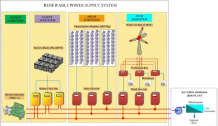
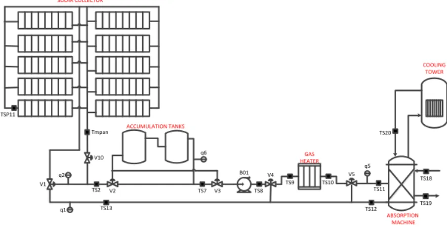
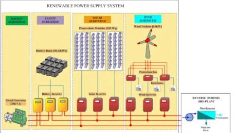
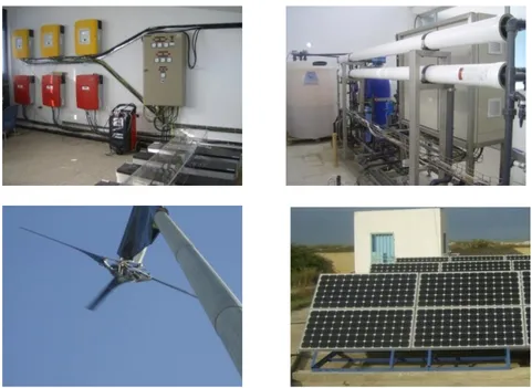
(23) Chapter 1. Introduction. 23. hydride metal storage) and renewable energy sources (photovoltaic panels and wind turbines). The aim is to guarantee electric energy for the local loads by keeping a balance between the consumed power and the produced power in spite of possible disturbances (s. Figure 1.1 and Figure 1.2 for the two systems considered).. Figure 1.1.- Solar, Wind and battery based Microgrid. Solar Panels. Battery Bank. Household. Ppv. Pload. Pbat. δez Pez. δfc Pfc Electrolyzer. Pgrid Grid. Fuel Cell. Metal Hydride Storage. Figure 1.2.- Solar and Hydrogen - based Microgrid. The second system considered focuses on thermal energy with the aim of providing water flow within a specific range of temperatures. The heat supply system comprises solar collectors as the renewable energy source, a gas heater, and storage tanks to store the extra energy generated by the solar collectors (s. Figure 1.3)..

(24) Chapter 1. Introduction. 24. In both cases, the main objective of the Energy Management System to be developed is to reduce the energy consumption from conventional energy sources, fulfill the operational constraints, not to decrease the lifetime of the installation, and ensure an efficient use of storage devices. SOLAR COLLECTOR. COOLING TOWER. TSP11 ACCUMULATION TANKS. Tmpan. TS20 q6. V10. GAS HEATER B01. q2. TS9. V1. TS2 q1. V2. TS7. V3. q5 V5. V4. TS18. TS10. TS8. TS13. TS11 TS19. TS12 ABSORPTION MACHINE. Figure 1.3.- Solar Gas Air Conditioning Plant. As is well known, storage devices are essential for the stable operation of the supply system. Considering traditional control strategy, the required capacity of this storage unit progressively increases as more and more energy sources are connected to the system. However, storage devices are expensive. As a result, one of the aims included in the proposed control is related to the efficient use of the energy stored in storage devices. Thus, the capacity of the storage unit does not depend on the number of energy sources connected to the systems. Additionally, it is recommended that the proposed controller should be able to predict the dynamic behavior of the system, due to the short-term unreliability of the renewable energy sources, and it should be computationally simple for online implementation. Model Predictive Control (MPC) has been chosen as it can handle variations in the supply of renewable energy and in the energy demand. It includes a cost function that can be written in economic terms, and operating constraints on the manipulated and controlled variables can be easily included in the control law. The process model must represent the process dynamic; it must predict the output signal with reasonable accuracy as well as being simple, because the future control actions computed by the optimizer take into account the integration of the model along the prediction horizon each sampling time. For MPC implementation, the main difficulty in the mentioned energy supply systems is in describing their dynamics, as this corresponds to a combination of differential equations and logic rules, in what is called hybrid systems. The usual.

(25) Chapter 1. Introduction. 25. approach for dealing with these hybrid process models, considered MPC, is the Mixed Logical Dynamic (MLD) framework, which allows the evolution of continuous variables to be specified through linear dynamic equations, the discrete variables to be specified through propositional logic statements, and the mutual interaction between both of them. As this optimization results in mixed integer quadratic programming (MIQP), it presents some problems for real time implementation, since the solution is computationally complex and depends exponentially on the number of binary manipulated variables. This limits the scope of application of MLD to very slow systems, since, for real time implementation, the sampling time would have to be large enough to allow the worst case computation. Thus, in this thesis, the hybrid MPC problem is transformed into a computationally simple problem which can be applied to the target systems.. 1.1.1.- Electrical energy supply system Most of the results on the control of wind and solar systems have focused on separate wind and solar systems. Specifically, there is a significant body of literature dealing with the control of wind-based energy generation systems (see, for example, Novak et al. [1], Chinchilla et al. [2] and Khan et al. [3] for results and references in this area), while several contributions have been made to the control of solar-based energy generation systems (see, for example, Johansen et al. [4], Camacho et al. [5] and Hamrouni et al. [6]). Currently, significant attention is being given to the development of supervisory control systems for hybrid generation systems that take into account maintenance and optimal operation considerations. One solution focuses on the design of PI controllers to regulate the output power of each source with the aim of keeping the grid frequency close to the nominal value, considering that the grid frequency deviates for sudden changes in load or generation. However, the use of a conventional PI controller does not meet the requirements of robust performance. For this, a technique has been proposed to tune the controller gains using Particle Swarm Optimization (PSO) in Si et al. [7], or using gain scheduling techniques combined with fuzzy control (Kakigano et al., [8]). In 2013, Keyrouz et al. presented a multidimensional MPPT controller to search for and maintain operation at the maximum power point for a distributed hybrid energy system based on the irradiance, temperature and wind speed. The controller is based on the fusion of two algorithms, namely the improved PSO and IncCond, using a Bayesian fusion. This novel fusion-based method was proved to be superior to a PSO-based technique and boosted the overall efficiency of the system, even under changing weather conditions (Keyrouz et al., [9]). Additionally, Weiss presented a fuzzy control to perform the standard power insertion into the line on the principle of maximum tracking (Weiss et al., [10])..

(26) 26. Chapter 1. Introduction. The MPPT controller is only recommended for supply energy systems connected to the main grid, due to the fact that the controller always tries to achieve the maximum power of the renewable source (Hussein et al., [11]). As a result, if the supply energy system is connected to a specific load, the controller is not able to limit the output power of the renewable source when the storage devices are fully charged and an excess energy is presented. In 2012, Zhang et al. introduced an energy management strategy based on power flow control for off-grid systems, with the aim of maintaining the state of charge (SOC) of the batteries within a certain range and avoiding over-discharge, over-charge and reducing the transitions between charge and discharge through power limitation of sources and loads (Zhand et al., [12]). In 2011, Qi et al. proposed a supervisor predictive control system which coordinates the renewable sources as well as a storage device to provide enough energy to satisfy the power demand. In the supervisory MPC, a specific cost function is designed to take into account the desired control objective (Qi et al., 2011 [13]). The supervisory MPC optimizes the output power from renewable energy and tries to reduce short term charge and discharge cycles of the storage device. Considering all manipulated variables are continuous, the MPC problem results in a problem of nonlinear optimization with continuous variables (NMPC). Unfortunately, the studied supply energy system does not include a backup subsystem, such as a diesel generator; in consequence, when the renewable energy is not sufficient and the storage devices are empty, the load must be disconnected, which is not recommended. Once again, in 2013, Qi et al. proposed a supervisory predictive control for a system made up of a wind subsystem, a solar subsystem and a battery bank associated to each renewable source (Qi et al., 2013 [14]). In this case, the energy supply system has the possibility of being connected to the main grid; as a result, it is not necessary to disconnect the load when the renewable energy is not sufficient and the batteries are empty. The centralized supervisory MPC controller, proposed above, is replaced with two distributed supervisory MPC controllers, each of which is responsible for providing optimal reference trajectories to the local controller of each corresponding subsystem. The distributed supervisory controllers are interconnected, so the measurements related to the wind/solar subsystem, the forecast of the future power demand and the weather forecast, are all available to both controllers.. 1.1.2.- Thermal energy supply system For solar thermal systems, most of the proposed control strategies focus on solar collector fields. In this case, the main control requirement is to maintain the outlet temperature of the collector field at a given value. However, this aim can only be achieved through mass flow adjustment, since the solar irradiation cannot be manipulated, and changes substantially during operation. As a result, significant.

(27) Chapter 1. Introduction. 27. variations are presented in the dynamic characteristics of the field and a satisfactory performance is difficult to obtain with a linear controller of fixed parameters. A self-tuning controller for a solar distributed collector field, based on a pole assignment approach which employs serial compensation to cope with measurable external disturbance, was presented by Camacho et al. [15]. Self-tuning control offers an approach by which the controller parameters of the model can be adjusted during operation to compensate for changes in the dynamic characteristics of the field and thereby maintain the desired control performance. Pickhardt et al. [16] proposed a nonlinear control based on predictive control with a mathematical input-output model of the plant, which was used for the distributed collector field of a solar power plant. The proposed controller is considered an indirect adaptive controller, since the model could change at every sampling instant. The nonlinear model adopted was assumed to be one of a “time invariant” nature. Henriques et al. [17] proposed a hierarchical control strategy based on a PID with a fuzzy logic switching supervisor. The supervisor was derived to implement the on-line switching between each PID controller, according to the measured conditions. The local PID controllers have been previously tuned off-line, using a neural network approach that combines a dynamic recurrent non-linear neural network model with a pole placement control design. A c-Means clustering technique was applied to reduce the number of local controllers. Johansen et al. [18] proposed and tested a control strategy based on switching between multiple local linear models/controllers. For this, the application of gainscheduled control was tested in a pilot-scale solar power plant. It was shown that the gain-scheduling can effectively handle plant nonlinearities, using high-order local linear ARX models that form the basis for the design of local linear controllers using pole placement. Stirrup et al. [19] proposed a control scheme that employed a fuzzy PI controller with feed forward for the highly nonlinear part of the operating regime, and gain scheduling control over the linear part of the operating envelope. Johansen et al. [4] proposed a control scheme based on a PID with time varying nonlinear gain, together with a feed forward controller. In this case, the internal energy was used as feedback instead of the outlet temperature of the solar collector. It was shown that the dynamics of the internal energy are simple compared to the dynamics of the outlet temperature. Stirrup et al. [20] proposed a hybrid controller for a solar thermal power plant using a gain scheduled controller with feed forward to control the more linear operating regimes and a fuzzy PI incremental controller for the highly nonlinear operating region of the plant..

(28) 28. Chapter 1. Introduction. Farkas et al. [21] developed a simplified physically-based model on the basis of energy balances, including solar irradiation as an input, using heat transferred by the flow of the water as a working medium, and overall heat loss from the plant. Average outlet temperature of the collector field is the reference value. A robust internal model-based controller IMC was applied for temperature control. Another thermal energy supply system considered in the literature comprises renewable and conventional energies, given by a solar collector field and a gas heater. Additionally, difficulties arise from the presence of discretely switched valves and continuous manipulated variables, which make it a hybrid system. The main control goal for this process is to minimize the consumption of auxiliary energy while ensuring a safe and robust operation, even in the face of large disturbances. Engell [22] presented a supervisory control scheme that switches the discrete inputs of the solar plant according to logic conditions defined over the measurements of process variables. In each mode, the continuous inputs are set to constant values that ensure a safe process operation, while keeping the energy losses to the environment small and minimizing the consumption of auxiliary energy. Zambrano et al. [23] proposed a hierarchical structure composed of two main levels, namely the configuration and the regulatory control levels. The configuration level selects the operating mode by means of minimizing a linear function with variable weights. The weights assigned depend on the current state of the plant and on the weather conditions, while the regulatory control level adjusts the variables of the process related to each operating point by using model predictive control in several structures of control loops. Rodríguez et al. [24] developed a model predictive control strategy with the aim of dealing with the mixed discrete-continuous nature of the process. For this, an internal model with embedded logic control is used to transform the hybrid problem into a continuous-nonlinear problem, so NMPC can be applied.. 1.2.- Model Predictive Control (MPC) Predictive Control refers to a set of control methods which use a process model to obtain the sequence of future control signals by minimizing an objective function. These control methods have basically the same structure and the same elements: they use a process model to predict the output signals, computing a control signal sequence by minimizing an objective function, and they use a receding strategy, where the horizon is moved toward the future at each sampling time and only the first control signal of the sequence computed at each step is applied. These control methods differ amongst themselves in the model structure used to represent the process, the noises and the cost function to be minimized..

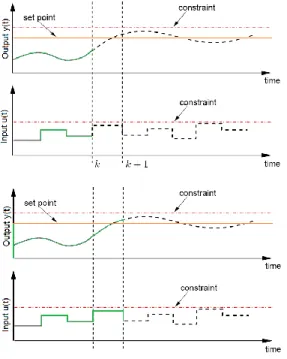
(29) Chapter 1. Introduction. 29. The methodology of Predictive Control methods is characterized by the following strategy, shown in Figure 1.4, (Camacho et al., [25], Keyser, [26]):. Figure 1.4.- MPC Strategy. | ) for a specific horizon N are 1) The future outputs of the process ̂( predicted at each sampling time t, considering the process model, the | ). known inputs and outputs, and the future control signals ( | ) is computed by 2) The sequence of future control signals ( optimizing a cost function defined to keep the process as close as possible ). This function usually takes the form to the reference trajectory ( of a quadratic function of the differences between the predicted output signal and the reference trajectory. An explicit solution can be obtained if the function cost is quadratic, the model is linear and there are no constraints. An iterative optimization method can alternatively be used. 3) The first control signal of the sequence computed at each sampling time ( | ) is sent to the process. A new control signal sequence ( | ) will be computed at the next instant: the control signal ( | ) might be different from the ( | ), as it considers the ). new information available, such as the measured output ( The structure shown in Figure 1.5 is used to implement the algorithm. Notice that a process model is used to predict the future outputs, based on the known past.

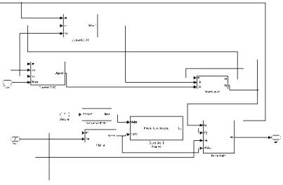
(30) Chapter 1. Introduction. 30. and current values and the future control actions. These actions are computed by the optimizer based on the cost function and the constraints. To do so, the internal model must adequately represent the process dynamics; it must predict the output signal accurately, as well as being simple. Past Inputs and Outputs. Predicted Outputs. Model. Reference Trajectory. +. -. Future Inputs. Optimizer Cost Function. Future Errors. Constraints. Figure 1.5.- MPC Strategy. Predictive Model | ) requires a process Computing the predicted output at future instants ̂( model. There are a variety of methodologies to obtain this model. Thus, considering the model structure, some control methods can be distinguished: Dynamic Matrix Control (DMC) (Cutler et al., [27]), Model Predictive Heuristic Control (IDCOM) (Richalet et al., [28]), Predictive Functional Control (PFC) (Richalet et al., [29]), Extended Prediction Self Adaptive Control (EPSAC) (Keyser et al., [30]) and others. Objective Function In Predictive Control, the aim is that the future outputs ̂ follow a determined reference signal during the considered horizon without excessive control efforts () ( ). The general expression is given by (1.1). J ( N1 , N 2 , N u ) . Nu. N2.   ( j)[ yˆ (t  k t )   (t  k )]    ( j)[u(t  k  1)] 2. k  N1. k 1. 2. (1.1). The following parameters can be used as tuning parameters to cover a wide scope of options: (i) Nu is the control horizon. (ii) N1 and N2 are the minimum and maximum prediction horizons that indicate the limits in which it is desirable for the prediction of the output to follow the reference. (iii) The coefficients δ(j) and λ(j) are weighting functions (usually constant values or exponential sequences). Obtaining the Control law | ), the cost function J To obtain the sequence of future control signals ( is minimized. An explicit solution can be obtained for the future control signal when the cost function is quadratic, the model is linear and there are no constraints;.

(31) Chapter 1. Introduction. 31. otherwise, an iterative method of optimization should be used. Whatever the method, obtaining the solution is not easy because there will be N2-N1+1 independent variables, a value which can be high. In order to reduce the degrees of freedom, a certain structure may be imposed on the control law by considering that, after a certain interval Nu, there is no variation in the proposed control signals or they are a linear combination of predetermined base functions (Richalet, [31]). Reference Trajectory One of the advantages of predictive control is that when the future evolution of the reference is known a priori, the system can react before the change has been applied, thus compensating for delays in the process response. Constraints All processes are subject to constraints: the actuators have a limited range of action and a limited slew rate, while the output variables are also limited for safety reasons. For this, the prediction capabilities of the MPC control make it possible to anticipate violations of the constraints and correct them by incorporating constraints into the cost function to be minimized (Maciejowski, [32]). Thus, bounds in the amplitude and slew rate of the control signal, as well as limits in the output, are all considered in the optimization. However, other types of constraints could be incorporated into the objective function, such as when the output variables are forced to have certain characteristics: band constraints, overshoot constraints, monotonic behavior, non-minimum phase behavior, actuator nonlinearities. Depending on the importance of the constraints, they are classified as hard constraints, relaxable hard constraints or soft constraints. Feasibility An optimization problem is infeasible when the region defined in the decision variables by the set of constraints is empty; as a result, the optimization does not have any valid solution. In contrast, it is feasible when there are points in the space of the decision variables that fulfill all the constraints. Notice that feasibility is of great importance for the stability proofs of constrained MPC. Some techniques for improving feasibility can be classified into: disconnection of the controller, constraint elimination, constraint relaxation and changing the constraint horizons. Predictive controllers present some drawbacks, such as: a). A process model has to be identified. For this, a significant amount of plant tests are required.. b) The tradeoff between tuning parameters and closed loop behavior is not evident. Tuning in the presence of constraints may be difficult, and even for the nominal case, it is not easy to guarantee closed loop stability, which is why so much effort is spent on simulations..

(32) Chapter 1. Introduction. 32. c). In order to speed up the solution time, several packages provide suboptimal solutions to the minimization of the cost function. It can be accepted in high speed applications, but is difficult to justify for process control applications unless the suboptimal solution is always very nearly optimal (Scokaert et al. [33]).. d) A systematic analysis of the stability and robustness properties of MPC is not possible in its original finite horizon formulation. The control law is in general time-varying and cannot be represented in the standard closed loop form, especially in the constrained case. For this, some formulations of predictive control have been proposed that ensure closed loop stability (Chen et al. [34]).. 1.3.- Nonlinear Predictive Control Many processes are nonlinear with varying degrees of severity. Sometimes, the process operates within the neighborhood of a steady state, and therefore a linear representation is adequate; although there are some very important situations where the linear representation is not good. On the one hand, there are processes with severe nonlinearities which are crucial to the closed loop stability, where a linear model is not sufficient. On the other hand, there are some processes that experience continuous transitions and spend a great deal of time away from a steady state operating region, or even processes which are never in steady state operation. For these processes, a linear control law will not be very effective, so nonlinear controllers will be essential for improved performance or simply for stable operation. Mathematical Formulation of NMPC A mathematical formulation of NMPC will be described considering a nonlinear continuous model represented by the nonlinear differential equation (1.2) and (1.3).. x (t )  f ( x(t ), u(t )), y(t )  g ( x(t ), d (t )). x(0)  xo. (1.2) (1.3). Here x(t), y(t) and u(t) denote the vector of states, outputs and inputs, respectively. Additionally, the output and input constraints are given by (1.4), (1.5) and (1.6).. . . Y : y  y  y ,. (1.4).

(33) Chapter 1. Introduction. 33.   D : u  u  u,. U : u  u  u ,. (1.5) (1.6). In NMPC, the input applied to the system is usually given by the solution of the following finite horizon open-loop optimal control problem, which is solved at every sampling instant, as shown in (1.7). Nu. J    ( j )[ yˆ (t   t )   (t   )]2 d   ( j )[u (t  k  1)]2 N2. N1. k 1. (1.7). Both the vector of states x and outputs y include continuous variables; as a result, an integral was used instead of the summation for the first term in the cost function, while u is considered a discrete variable due to its value being constant at ). Finally, the optimization problem at each sampling instant can be expressed as (1.8), subject to (1.9), (1.10), (1.11), (1.12) and (1.13).. min. u ( k ),, u ( k  N u 1) Nu. J    ( )[ yˆ (t   t )   (t   )]2 d   (k )[u (t  k  1)]2 N2. N1. (1.8). k 1. x(t   t )  f (x(t    1t ), u(t   t ))   [1, N 2 ]. (1.9). yˆ (t   t )  g (x(t   t ), d(t   t )).   [1, N 2 ]. (1.10). u(t  k  1t )  D. k  1,, Nu. (1.11). u(t  k t )  U. k  1,, Nu. (1.12). yˆ (t   t )  Y.   [ N3 , N 4 ]. (1.13). The output vector predictions are obtained by solving differential and algebraic equations for different control laws defined in each sampling instant. N3 and N4 is the range where output constraints are applied. Notice 1≤ N3≤N4≤N2 If the numerical integration of the differential and algebraic equations is used, it will be necessary to include a new element in the predictive control scheme: a simulation Package. This is known as the direct method for solving dynamic.

(34) Chapter 1. Introduction. 34. | ), optimization problems. The optimizer will define a control law ( j=1...Nu at each sampling instant. The current state of the process, together with the control law, will be used for the simulation package to simulate the model (i.e.: integrate the dynamic equations) and obtain a value for the cost function. Afterwards, the optimizer will define a new control law, the dynamic of the process | ), a new will be simulated again considering this new control law ( value for the cost function will be reached, and so on until an optimal control law which minimizes the cost function has been found. This control law will eventually be applied to the process, based on the receding prediction horizon. Including a simulation package to simulate the dynamic of the process in which the model is programmed allows the use of nonlinear models as complicated and/or detailed as desired, making different formulations of the same models possible. The main drawback is the computational cost associated to the integration of large and complex models. This predictive control formulation, based on nonlinear and continuous models in which the process model is integrated by means a simulation package, to obtain a value of the cost function at the end of the prediction horizon, together with discrete events, will be the basic idea followed in the following sections.. 1.4.- Outline of the Chapter The remainder of this thesis is organized as follows. In Chapter 2, the implementation of MPC considering a three blade wind turbine is described. As a result, a review of the dynamic model and the traditional control strategy associated with the wind turbine are also discussed. The developed predictive control for hybrid systems is implemented considering the energy supply system studied in Chapter 3. The integrated system includes a Reverse Osmosis (RO) desalination unit and a three-phase power supply system comprising PV modules, a wind turbine, a battery bank and a diesel generator. Additionally, a MATLAB simulation platform was built considering the dynamic models of each energy source. Simultaneously, the internal model used for the proposed predictive control will be based on the simulation platform. Chapter 4 presents the development of a simulation model for a solar gas airconditioning plant with the aim of providing a suitable temperature inside a building during the hot season with minimum energy consumption. The plant is made up of three main sections: the refrigeration system, the single – effect LiBrH2O absorption machine and the solar heat supply system. However, the proposed controller is focused on the solar heat supply system, which provides a hot water flow to the generator of the absorption machine and is composed of three main.

(35) Chapter 1. Introduction. 35. elements: a solar collector field, an ON/OFF gas heater and two thermally isolated accumulation tanks. Chapter 5 includes a review of a hydrogen based MicroGrid made up of a PEM electrolyzer, a metal hydride storage, a PEM fuel cell, a battery bank, PV modules and an electronic load. The main objective is to fulfill the local loads by keeping a balance between the consumed and the generated power, in spite of possible ambient disturbances. A central aspect in the optimization of the energy storage is the consideration of its energy requirements. The metal hydride is used to provide energy for long term requirements, while the battery bank is used for the short term. This implies guaranteeing a good behavior of the fuel cell and electrolyzer so as not to reduce the lifetime of the components. Both the aim and the constraint will be taken into account in the proposed MPC control. The conclusions contain a detailed discussion of the systems‟ behavior and are made comparing the simulation and experimental results with the theoretical analysis. Finally, potential future work is discussed.. 1.5.- Summary of Publications This thesis is based on submitted articles: . J. Salazar, F. Tadeo, C. de Prada and M. Chaabane. “Modeling of MicroSource for Microgrid during Island Operation”, 2nd Int. Conf. on Communications, Computers and Control Applications (CCCA`12), Marseille, France, 6-8 Dec. 2012.. . J. Salazar, F. Tadeo, C. de Prada and L. Palacin. “Modeling and control of a wind turbine equipped with a permanent magnet synchronous generator (PMSG)”, 22nd European Modeling & Simulation Symposium, FES, Morocco, October 13-15, 2010.. . J. Salazar, J. D. Álvarez Hervás, J. L. Guzmán and F. Tadeo, “Controloriented Modelling of the Solar Climatization of a Public Building in Mediterranean Climate”, Conférence and Exposition Internationales Vehicules Écologiques and Énergies Renouvalables, Monaco, Monaco, March, 2013.. . J. Salazar, F. Tadeo and C. Prada. “Renewable Energy for Desalinization using Reverse Osmosis”, International Conference on Renewable Energies and Power Quality (ICREPQ’10), Granada, Spain, 23th to 25th March, 2010..