TítuloTime averaged shallow water model: asymptotic derivation and numerical validation

Time-averaged shallow water model: asymptotic derivation and

numerical validation

∗

J. M. Rodr´ıguez

R. Taboada-V´

azquez

Abstract

The objective of this paper is to derive, from the Navier-Stokes equations in a shallow domain, a new bidimensional shallow water model able to filter the high frequency oscillations that are produced, when the Reynolds number is increased, in turbulent flows. With this aim, the non-dimensional Navier-Stokes equations are time-averaged, and then asymptotic analysis techniques have been used as in our previous works (Rodr´ıguez and Taboada-V´azquez 2005-2012 [17]-[23]). The small non-dimensional parameter considered,ε, is the quotient between the typical depth of the basin and the typical horizontal length of the domain; and it is studied what happens when ε becomes small.

Once the new model has been justified, by the method of asymptotic expansions, we perform some numerical experiments. The results of these experiments confirm that this new model is able to approximate analytical solutions of Navier-Stokes equations with more accuracy than classical shallow water models, when high frequency oscillations appear. To reach a given accuracy, the time step for the new model can be much larger (even four hundred times larger) than the time step required for the classical models.

Keywords: Shallow waters, Asymptotic analysis, Reynolds Averaged Navier-Stokes equations (RANS), Large Eddy Simulation (LES), Modelling, Filtering.

MSC 2010: 35Q35, 35Q30, 76D05, 41A60, 76M45, 76F65.

1

Introduction

As it is well known, the equations governing the behavior of a fluid are the Navier-Stokes equations. Due to their strong nonlinearity, high frequency oscillations are produced when the Reynolds number is increased, and the flow becomes unstable and turbulent. It is computationally very expensive to solve the equations directly, so at the moment, the most common approach in hydraulic engineering practice is to solve the Reynolds Averaged Navier-Stokes equations, in which the effect of turbulence is modelled rather than solved.

We approximate Navier-Stokes equations using a shallow water model, but if the flow is turbulent, a very small time step must be chosen. This paper is focused on the derivation of a new bidimensional time-averaged shallow water model able to reduce these oscillations, and then able to achieve good results with larger time steps.

Filtering has given good results when working with turbulent Navier-Stokes equations (see [24]). In the literature, we can found that the separation between large and small scales is traditionally assumed to be obtained by applying a spatial filter to the Navier-Stokes equations (see [3, 12]); but time filtering is also suggested by several authors (see [4, 16]). In this work, we shall use a time filter, thus avoiding to model the spacial filtered stress tensor (see [3]).

Asymptotic analysis has been applied successfully to derive and justify shallow water models. The new model, developed from the incompressible Navier-Stokes equations with free surface, has been deduced

∗_{This work has been partially supported by MTM2012-36452-C02-01 project of Ministerio de Econom´ıa y}

Competitivi-dad of Spain with the participation of FEDER.

†_{Department of Mathematics and Representation Methods, College of Architecture, University of A Coru˜na, Campus}

da Zapateira, 15071-A Coru˜na, [email protected]

‡_{Department of Mathematics and Representation Methods, School of Civil Engineering, University of A Coru˜na, Campus}

in the spirit of the method proposed in our previous works [17]-[23] and [25]. In order to obtain a shallow water model, we consider a domain with small depth compared with its other dimensions. We use in the sequel the thin-layer assumption and introduce a “small” non-dimensional parameterε=HC/LC where HC andLCare, respectively, the typical scales for the vertical and the horizontal dimensions of the fluid

domain of interest.

The outline of the paper is as follows. In the next section we introduce and render non-dimensional the model that serves as our starting point. Then, the time averaging process is described in section 3 and asymptotic analysis is applied following the ideas of [17]-[23] (section 4) to derive our shallow water model that is presented in section 5. We show, in section 6, that this new model is able to obtain a given accuracy using time steps larger than the time steps needed by classical shallow water models. Finally, we make some concluding remarks in section 7.

2

The three-dimensional model equations

In this section we present the three-dimensional incompressible Navier-Stokes model that serves as the starting point for our subsequent development. The first subsection gives the basic mass and momentum balance laws for a basin with varying bottom topography and a free top surface, and supplements them with appropriate boundary conditions. In subsection 2.2 we introduce the shallow water scaling, define a non-dimensional parameter and non-dimensionalize the three-dimensional model in terms of that parameter.

2.1

Three-dimensional incompressible flow

Let us start with the Navier-Stokes system [13] for incompressible homogeneous fluids, with gravity and Coriolis force, evolving in a sub-domain of R3_{. As the domain, the functions and variables involved}

in this problem depend on ε, we indicate this dependence with superscript ε. Therefore, we have the following general formulation expression:

∂ ⃗Uε

∂tε +

(

⃗ Uε· ∇ε

)

⃗

Uε=−1

ρ0∇

ε_Pε_+ν∆ε_U⃗ε_+F⃗ε

e (1)

divU⃗ε= 0 (2)

and we consider this system for

tε∈[0, T], (xε, yε)∈D⊂R2, Bε(xε, yε)≤zε≤Sε(tε, xε, yε)

where:

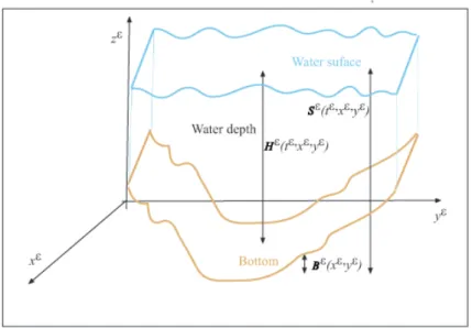
• Sε_(tε_{, x}ε_{, y}ε_{) represents the free surface elevation (unknown) and B}ε _{the bathymetry (it is not}

constant and it is supposed to be known). The water height isHε=Sε−Bε(see Figure 1)

• _U⃗ε_{= (U}ε

1(tε, xε, yε, zε), U2ε(tε, xε, yε, zε), U3ε(tε, xε, yε, zε)) is the three-dimensional velocity of the

fluid

• Pε_(tε_{, x}ε_{, y}ε_{, z}ε_{) is the pressure} • ρ0 denotes the density of the fluid • ν is the kinematic viscosity

• _F⃗ε

e=−g⃗k−2Φ⃗ ×U⃗ε is the volume force per unit mass, whereg is the gravitational acceleration

(assumed constant) and −2⃗Φ×U⃗ε is the Coriolis acceleration (where the angular velocity of

rotation of the Earth is ⃗Φ = Φ

(

sinφ⃗k+ cosφ⃗ȷ

)

with Φ = 7.29×10−5 _{rad/s;⃗ı,⃗ȷ and}⃗_{k denote}

Figure 1: Notations: water heightHε_(tε_{, x}ε_{, y}ε_{), free surfaceS}ε_(tε_{, x}ε_{, y}ε_{) and bottomB}ε_(xε_{, y}ε₎

The kinematic continuity condition

U₃ε=∂H

ε

∂tε +U

ε 1

∂Sε

∂xε +U

ε 2

∂Sε

∂yε atz

ε_=Sε_(tε_{, x}ε_{, y}ε_{) (3)}

is rewritten in equivalent form (for incompressible fluids):

∂Hε

∂tε +

∂ ∂xε

∫ Sε

Bε

U₁εdzε+ ∂

∂yε

∫ Sε

Bε

U₂εdzε= 0 (4)

Equations (1)-(2) must be supplemented by boundary conditions.

• At the bottom,

– the non-penetration condition is satisfied:

⃗

Uε·⃗nε= 0 atzε=Bε(xε, yε) (5)

where⃗nε_{denotes the outward unit normal to the boundary of the domain.}

– tangential forces must be equal to the friction force:

(I−⃗nε⊗n⃗ε)Tε⃗nε=⃗Fε_R atzε=Bε(xε, yε) (6)

Typically, the friction force per unit of surface area is of the formF⃗ε

R =−ρ0CRε|U⃗

ε_|U⃗ε _(Cε R

is small), see for example [7] or [26].

• On the free top surface we assume that the only external force acting on the fluid is the wind stress. In particular, we assume that the surface tension and ambient atmospheric pressure variations are negligible. This leads to the boundary condition

Tε⃗nε=−P_sε(tε, xε, yε)⃗nε+F⃗ε_W atzε=Sε(tε, xε, yε) (7)

where ⃗Fε_W is the force of the wind and P_sε is the atmospheric pressure at the surface (supposed known).

The stress tensor (Tε_{) is given by:}

T_ijε =−Pεδij+µ

(

∂Uε

i ∂xε j

+∂U

ε j ∂xε i

)

i, j= 1,2,3 (8)

wherexε₁=xε,xε₂=yε,xε₃=zε,µ=ρ0ν is the dynamic viscosity andδij is the Kronecker’s delta.

2.2

Non-dimensionalization

The shallow water approximation is characterized by the smallness of a non-dimensional parameter that we can identify assuming that the typical depth of the basin (HC) is much smaller than the typical

horizontal length (LC), i.e., that

HC

LC

=ε where ε <<1 (9)

This small parameter is an aspect ratio.

We introduce the non-dimensional independent variablest,x, yandz by

t= t

ε

TC

, x= x

ε

LC

, y= y

ε

LC

, z= z

ε

εLC

(10)

where TC is a typical time. Recalling (9), the non-dimensional water height and bottom surface are

defined by

h(t, x, y) = H

ε_(tε_{, x}ε_{, y}ε₎

εLC

, b(x, y) =B

ε_(xε_{, y}ε₎

εLC

(11)

so the non-dimensional top surface is given by

s(t, x, y) =S

ε_(tε_{, x}ε_{, y}ε₎

εLC

(12)

We shall now introduce non-dimensional functions and constants:

uεi(t, x, y, z) =

TC

LC

Uiε(tε, xε, yε, zε), i= 1,2,3 (13)

pε(t, x, y, z) = T

2 C ρ0L2C

Pε(tε, xε, yε, zε), ps(t, x, y) = T2

C ρ0L2C

P_sε(tε, xε, yε) (14)

G= T

2 C

LC

g, ϕ=TCΦ (15)

σ_ijε(t, x, y, z) = T

2 C ρ0L2C

T_ijε(tε, xε, yε, zε) i, j= 1,2,3 (16)

⃗

f_Wε = T

2 C ρ0L2_C

⃗

Fε_W, f⃗_Rε = T

2 C ρ0L2_C

⃗

Fε_R (17)

where we have assumed thatpsdoes not depend onε.

2.2.1 The non-dimensional equations

We now express the three-dimensional incompressible Navier-Stokes system (1), (2) and (4) in terms of the above non-dimensional variables and functions:

∂uε 1

∂t +u

ε 1

∂uε 1

∂x +u

ε 2

∂uε 1

∂y +

1

εu

ε 3

∂uε 1

∂z =−

∂pε

∂x +

1

Re

(

∂2_uε 1

∂x2 +

∂2_uε 1

∂y2 +

1

ε2

∂2_uε 1

∂z2

)

+ 2ϕ((sinφ)uε2−(cosφ)u ε

3) (18)

∂uε 2

∂t +u

ε 1

∂uε 2

∂x +u

ε 2

∂uε 2

∂yε +

1

εu

ε 3

∂uε 2

∂z =−

∂pε

∂y +

1

Re

(

∂2_uε 2

∂x2 +

∂2_uε 2

∂y2 +

1

ε2

∂2_uε 2

∂z2

)

−2ϕ(sinφ)uε1 (19)

∂uε3

∂t +u

ε 1

∂uε3

∂x +u

ε 2

∂uε3

∂y +

1

εu

ε 3

∂uε3

∂z =−

1

ε ∂pε

∂z +

1

Re

(

∂2uε3

∂x2 +

∂2uε3

∂y2 +

1

ε2

∂2uε3

∂z2

)

−G+ 2ϕ(cosφ)uε₁ (20)

∂uε 1

∂x +

∂uε 2

∂y +

1

ε ∂uε

3

∂z = 0 (21)

∂h

∂t +

∂ ∂x

∫ s

b

uε₁dz+ ∂

∂y

∫ s

b

whereνTC L2 C

= 1

Re. The non-penetration condition (5) yields:

uε3=ε

The non-dimensional stress tensor can be written:

σε_ij =−pεδij+

so boundary conditions (6)-(7) result



3

Time averaging process

The formal derivation of our shallow water model has two steps. We first obtain the time-averaged Navier-Stokes equations and then make the shallow water approximation.

We define:

¯

If we assume that 0< η <<1, and we approximateuε_i by its Taylor’s expansion forr∈(t−η, t+η):

then we have:

¯

It is easy to demonstrate for regular enough functions fε and gε, and small enough η, that the following equalities are fulfilled:

∂fε

Applying (29), (32) and (34) to equations (18)-(21), they yield:

∂u¯ε

To average equation (22), in first place we writeuε

This averaging process provides from (23)-(27):

Condition (28) is time-averaged too and gives and similar but more complex expression, because s

depends ontand we need to use formula (35).

4

Asymptotic derivation of the shallow water model

After obtaining the time-averaged Navier-Stokes equations, we make the shallow water approximation by formally expanding solutions of the model in powers ofε.

4.1

Asymptotic expansion

Our shallow water model derive from the assumption that the aspect ratio ε is small. We make the shallow water approximation by formally expanding solutions of the model in powers of ε. We seek a formal solution in the form of an asymptotic series:

We substitute now this expansion into the system of equations (37)-(46), and grouping the terms multiplied by the same power ofε, we arrive at a series of equations that will allow us to determine ¯u0_i,

p0_{, etc. Let us show some particular examples.}

The value of ¯u0

3 can be found from the incompressibility condition (40) written at the leading order

O(ε−1_):

∂u¯0₃

∂z = 0⇒u¯

0 3= ¯u

0

3(t, x, y) (48)

We now consider the boundary condition (42); to the leading order it becomes:

¯

u03= 0 forz=b (49)

so

¯

u0₃= 0 (50)

In the same way, upon inserting the above expansion into (44), to order O(ε−1_{), one finds that}

∂u¯0 i

∂z = 0 i= 1,2 (51)

Now, incompressibility equation (40), to the leading orderO(1), gives

¯

u1₃=−

∫ z

b

(

∂u¯0 1

∂x +

∂u¯0 2

∂y

)

dz′+ ¯u1₃(t, x, y, b) (52)

and the boundary condition (42), together with the fact that ¯u01and ¯u02do not depend onz((51)), allows

us to write:

¯

u1₃= (b−z)

(

∂u¯0 1

∂x +

∂u¯0 2

∂y

)

+ ¯u0₁∂b

∂x + ¯u

0 2

∂b

∂y (53)

Equation (39), to orderO(ε−1), together with above expression for ¯u1₃, leads us to conclude that ¯p0 is constant with respect to the vertical variable:

∂p¯0

∂z =

1

Re ∂2u¯13

∂z2 = 0 (54)

and with the information that we obtain from boundary conditions we have:

¯

p0= ¯ps−

2

Re

(

∂u¯0 1

∂x +

∂u¯0 2

∂y

)

(55)

Equation (41), to the leading orderO(1), together with (51) becomes

∂h

∂t +

∂ ∂x

[

h

(

¯

u0₁−η

2

6

∂2_u¯0 1

∂t2

)]

+ ∂

∂y

[

h

(

¯

u0₂−η

2

6

∂2_u¯0 2

∂t2

)]

=O(η4) (56)

In summary, we are able to derive the following first terms and equations:

¯

u0₃= 0 (57)

¯

uk₃= (b−z)

(

∂u¯k₁−1

∂x +

∂¯uk₂−1 ∂y

)

+ ¯uk₁−1∂b

∂x+ ¯u

k−1 2

∂b

∂y, k= 1,2 (58)

¯

p0= ¯ps−

2

Re

(

∂u¯0₁

∂x +

∂u¯0₂

∂y

)

(59)

¯

p1= (s−z)(G−2ϕ(cosφ)¯u0₁)− 2

Re

(

∂u¯1 1

∂x +

∂u¯1 2

∂y

)

(60)

¯

σ0₁₃= ¯σ0₂₃= 0 (61)

∂u¯k₁

∂z =

∂u¯k₂

¯

4.2

First Order Approximation

We can now consider a first order approximation:

˜ of the vertical velocity and the pressure are:

˜

To obtain closed equations for ¯u0

1 and ¯u02we have to get rid of the terms ¯u21 and ¯u22in equations (63)

and (65). We can accomplish this with the following procedure. First integrate those equations in the vertical variablez fromb tos:

∂u¯0

∂z at the top surface and at the bottom. Using (70) and (58), we write:

∂u¯2_i

Next, substitutingzbysandb, we have:

To obtain the value of ¯σ_i1₃ at the top surface and at the bottom, boundary conditions (72), (73), (74) and (75) are used

∂u¯2

When we substitute expressions (85)-(86) into (81)-(82), we obtain

∂u¯0₁

We repeat the process from equations (64) and (66) to obtain closed equations for ¯u1

yield:

Equations (87)-(90) are used to obtain the following equations for ˜uε_i (see (77)):

∂u˜ε₂

The system of equations for ˜ui(i = 1,2) ((91)-(92)) is coupled with the following equation for the

water depth deduced from (67)-(68):

∂h

Therefore, if equations (91)-(93) are solved, we obtain the horizontal velocity and the free surface eleva-tion.

5

Proposed Shallow Water Model

In this section, we go back the original variables:

Hε(tε, xε, yε) =εLCh(t, x, y), Bε(xε, yε) =εLCb(x, y), (94)

and we present the model that we have derived. We begin summarizing the results that we have achieved in this theorem:

Theorem 1 Let us suppose that there exists asymptotic expansion (47). Then approximated solution (94)-(96) verifies

∂U⃗˜ε

We, finally, propose the following model that we have derived neglecting theO(ε2_{) andO(η}4_{) terms}

in the above equations. For notational convenience, we henceforth drop the˜.

∂Hε

Remark 1 In practice, we neglect the term inη2_{in equation (102), because it does not provide}

signifi-cant improvements in the accuracy of the numerical solutions that we present in section 6, but it causes some problems of stability. Therefore, in what follows, we replace (102) by

∂Hε

∂tε +∇

ε_·(_Hε_U⃗_¯ε)_{= 0 (106)}

6

Numerical experiments

asSW, and it can be written as in [18]:

∂Hε

∂tε +∇

ε_·(_Hε_U⃗ε)_{= 0}

∂ ⃗Uε

∂tε +∇U⃗

ε_·U⃗ε₌₋1 ρ0∇

Psε+ν{∆U⃗ε+

1

Hε[∇U⃗

εT _+∇U⃗ε_]∇Hε

+ 1

(Hε₎2∇[(H

ε₎2_{(∇ ·U⃗}ε_{)]} −g∇S}ε₊ 1 ρ0Hε

(

⃗

Fε_W +F⃗ε_R

)

+ 2Φ

{

(sinφ)

(

Uε

2 −Uε

1

)

+ (cosφ)

[

U1∇Sε+

1 2H

ε_∇(Uε 1) +

(

−_U⃗ε_{· ∇B}ε₊1

2H

ε_{∇ ·U⃗}ε

0

)]}

(107)

where the horizontal velocityU⃗ε_{is not averaged in time.}

In order to compare models (103)-(106) and (107), we shall consider some analytical solutions of Navier-Stokes equations ((1)-(8)) whose velocity rapidly oscillates in time. Then we solve numerically the equations (103)-(106) and (107) for the data provided by the analytical solutions of Navier-Stokes equations, and finally we compute the errors committed by each of the models.

To perform the numerical simulations, we have opted to use MacCormack scheme (see [14]) due to its good stability properties, its easy implementation, and to the fact that has been applied successfully to the resolution of similar problems.

Let us introduce now the first family of exact solutions to Navier-Stokes equations that we shall use to compare models SWand NM. Horizontal and vertical velocity oscillate in time, but the horizontal velocity depends on variablexε _{while the vertical velocity depends on variablez}ε_:

U1ε = (A1+A2xε) sin

(

2πn1

Tp tε

)

+ (B1+B2xε) cos

(

2πn1

Tp tε

)

+ (C1+C2xε) sin

(

2πn2

Tp tε

)

+ (D1+D2xε) cos

(

2πn2

Tp tε

)

U₂ε = 0

U₃ε = −zε

[

A2sin

(

2πn1

Tp tε

)

+B2cos

(

2πn1

Tp tε

)

+C2sin

(

2πn2

Tp tε

)

+ D2cos

(

2πn2

Tp tε

)]

Bε = 0

Hε = Ee

Tp

2π  A2

n1 cos

(_2πn

1

Tp tε

)

−B2

n1 sin

(_2πn

1

Tp tε

)

+C2

n2 cos

(_2πn

2

Tp tε

)

−D2

n2 sin

(_2πn

2

Tp tε

) 

P_sε = Pε(zε=Hε)−2µ∂U

ε 3

∂zε +F

ε W3

F_Wε

1 = F

ε W2= 0

⃗

F_Rε = ⃗0 (108)

where Ai, Bi, Ci, Di, ni(i = 1,2) and Tp are any real value. We are able to calculate an analytical

expression forPε_{from equation (1), but it is too long and we have decided not to include it here.}

We consider that D is a rectangular basin of length 10 meters and width 2 meters with a 100×20 points grid (that is, the discretization step used is ∆xε _{= ∆y}ε _{= 0.1). We choose the values of the}

parameters so the maximum depth is always smaller than 1 meter, and thus the aspect ratio is always smaller than 10−1_{. We solve in temporal interval [0,10] with different time steps.}

We introduce these two sets of values for the constants:

A1=B1= 2, C1=D1= 0.5, A2=B2=C2=D2= 0, E= 1 (109)

A1=B1= 1, C1=D1= 0.5, A2=B2= 0.5, C2=D2= 0, E= 0.75 (110)

and (107) with these choices of constants. For both examples we take: Φ = 0, g = 9.8, ρ = 998.2,

ν= 1.02×10−6,Tp= 1,n1= 0.1,n2= 100.

We remark that in model (103)-(106) we must chooseη andTC, whereTC is the characteristic time

and 2η is the length of the averaging interval for the non dimensional time variable; but the relevant choice here is the value of the productηTC because 2ηTC is the length of the averaging interval for the

dimensional time variable.

∆t Error bound Error bound Error bound Error bound forH SW forH NM forU1 SW for ¯U1 NM

0.01 0 0 3.1e3 9.7e−3 0.005 0 0 2.6e0 4.8e−3 0.001 0 0 4.0e−1 9.7e−4 0.0001 0 0 3.8e−2 9.7e−5 0.000025 0 0 9.5e−3 2.4e−5

Table 1: Error bounds for example (108) with data (109) andηTC = 2.5

In Table 1 we show the error bounds when comparing the computed solution ofSWwith the Navier-Stokes solution (108), and when comparing the computed solution of NM with the averaged version of (108). We can see that, to obtain the same order of accuracy than the new model (103)-(106) with ∆t = 10−2_{, model (107) has to be solved taking ∆t = 2.5×10}−5_{, that is, the time step must be 400}

times smaller. In this example, the depth is computed exactly by both models because it just depends on time.

The times (in seconds) required to solve modelsSWandNMfor the example of Table 1 are presented in Table 2. We have used for these computations a personal computer with an Intel(R) Core(TM) i5 2.80 GHz processor (6 Gb RAM). We can see in this Table 2 that execution time for the new model increased compared with model SW for the same time step, but we can observe that it is shorter if we want to obtain the same accuracy. For example in this case, using the new model, in 8.4 seconds we have a more accurate approximation of the solution than the one obtained with model SWin 268 seconds. We see that the time needed to achieve the same accuracy with (107) is 1073 seconds.

∆t= 10−2 _{∆t= 5×10}−3 _{∆t= 10}−3 _{∆t= 10}−4 _{∆t= 2.5×10}−5

SW 2.9 5.4 27.0 268.5 1073.0

NM 8.4 16.4 81.5 812.6 3284.9

Table 2: Execution times (in seconds) of the example of table 1

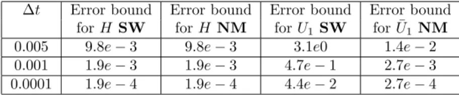
In Table 3 we observe that, when velocity depends on the spatial variable xε, the results achieved with the new model are quite better too. When we introduce data (110), we need to introduce a small value for η (ηTC = 5×10−3) to guarantee the convergence of the scheme for ∆t = 10−4. For larger

values of ∆t, it is possible to choose larger values ofη.

∆t Error bound Error bound Error bound Error bound forH SW forH NM forU1SW for ¯U1NM

0.005 9.8e−3 9.8e−3 3.1e0 1.4e−2 0.001 1.9e−3 1.9e−3 4.7e−1 2.7e−3 0.0001 1.9e−4 1.9e−4 4.4e−2 2.7e−4

Table 3: Error bounds for example (108) with data (110) andηTC = 5×10−3

0.0001 0.001 0.005 10−4

10−3 10−2 10−1

100

∆ t

Error bounds for example (108) with data (110) and η T_C=5 × 10−3

U₁ SW time−averaged U₁ NM

Figure 2: First order accuracy of the numerical scheme

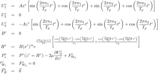
Let us consider now the following solution to Navier-Stokes equations where water depth depends on

xε_:

U₁ε = Axε

[

sin

(

2πn1

Tp tε

)

+ cos

(

2πn1

Tp tε

)

+ sin

(

2πn2

Tp tε

)

+ cos

(

2πn2

Tp tε

)]

U₂ε = 0

U₃ε = −Azε

[

sin

(

2πn1

Tp tε

)

+ cos

(

2πn1

Tp tε

)

+ sin

(

2πn2

Tp tε

)

+ cos

(

2πn2

Tp tε

)]

Bε = 0

Hε = B(xε)me

ATp(m+1) 2π

 cos

( 2πn1

Tp tε

)

−sin (

2πn1

Tp tε

)

n1 +

cos (

2πn2

Tp tε

)

−sin(2πn2

Tc tε)

n2

 

P_sε = Pε(zε=Hε)−2µ∂U

ε 3

∂zε +F

ε W3

F_Wε₁ = F_Wε₂ = 0

⃗

FRε = ⃗0 (111)

withm∈N,A,B,ni(i= 1,2) andTp any real value.

For the following values of the constants

A= 0.03, B= 0.1, n1= 0.1, n2= 100, Tp= 1, m= 1 (112)

time step must be very small (∆t= 10−4_{) to achieve the convergence of modelSWwhile the new model}

gives reasonable results with ∆t= 10−3 _{as we show in Table 4.}

∆t Error bound Error bound Error bound Error bound forH SW forH NM forU1SW for ¯U1NM

0.001 — 1.2e−2 — 2.1e−1 0.0001 7.2e−2 2.9e−3 3.6e−1 5.1e−2

Table 4: Error bounds for example (111) with data (112) andηTC = 1.3034×10−2

We can observe from Tables 3 and 4 that, when the solution depends on xε_{, we need to take small}

values of ηTC. This is due to the fact that approximation (31) (and, as consequence, all formula

0 0.5 1 1.5 2 2.5 3 3.5 4 4.5 5 5.5 −1.5

−1 −0.5 0 0.5 1 1.5

t x=8, y=0.5

U₁ SW (∆ t= 5 10−4)

time−averaged U₁ NM (∆ t=10−2)

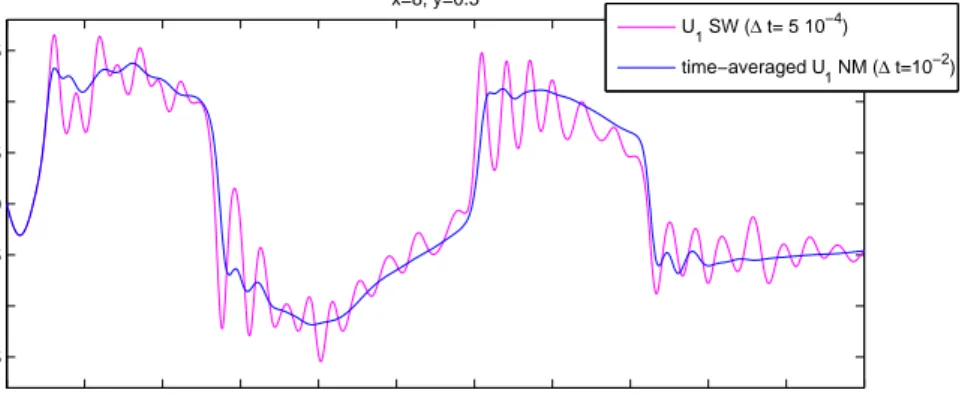
Figure 3: Comparison betweenU1 SWand ¯U1NM

Finally, we present a more realistic numerical experiment which does not give a precise solution of the Navier-Stokes equations. Zero-Dirichlet boundary conditions are imposed for horizontal velocity. At the initial time, horizontal velocity is set to be zero and the the water depth is:

H₀ε(x, y) =

  

1 + 0.1 sin(2πx) ifx∈[0,3)∪(7,10]

1.9 + 0.1 sin(2πx) if [3,7]

(113)

In this case, as we have already commented for the previous example, time step must be quite small (∆t= 5×10−4_{) to achieve the convergence of modelSWwhile the new model gives reasonable results}

even with ∆t= 10−2_{. We have plotted together, in figure 3, the approximations of theU}

1 component

of the horizontal velocity that both models provide. We observe that the new model reduces the high frequency oscillations that appear using the shallow water model. If we compare the execution times, we have that the time required to solve modelSW with this data is 45 seconds while modelNMruns in just 7 seconds.

7

Conclusions

We have used asymptotic analysis to obtain from the time-averaged non-dimensional Navier-Stokes equations a new shallow water model. The new model is able to filter (in some representative cases) the high frequency oscillations and this allows us to choose a much larger time step.

We have made some numerical comparisons between the new model and the shallow water model proposed in [17]. Numerical experiments confirm that this new model is able to obtain a given accuracy using larger time steps than the time step needed by the other shallow water model (see Tables 1, 3-4 and figure 3). In some cases, the time step can be even four hundred times larger. This enhancement leads to much shorter execution times compared with the execution times required by the classical shallow water model to obtain the same precision (see Table 2).

Although the numerical results achieved improve those of the model without time filtering, we have observed not so good results in some cases. We think that it can be caused by the absence of spacial filtering, and it would be convenient to use a combination of spacial and time filters, as suggested in [4], because the use of spacial “projective” filters or modelling of subgride-scale stress tensor is necessary to reduce the number of degrees of freedom of the problem.

References

[2] P. Az´erad, F. Guill´en, Mathematical justification of the hydrostatic approximation in the primitive equations of geophysical fluid dynamics,Siam J. Math. Anal.,33(4), 847–859, (2001).

[3] D. Carati, F.S. Winckelmans, H. Jeanmart, “On the modelling of the subgrid-scale and filtered-scale stress tensors in large-eddy simulation”, Journal of Fluid Mechanics, 441, 119-138, 2001.

[4] D. Carati, A.A. Wray, “Time filtering in large eddy simulations”, Proceedings of the summer Pro-gram 2000 Center for Turbulence Research, 263-270, 2000.

[5] E. Casas, Introducci´on a las ecuaciones en derivadas parciales, Universidad de Cantabria, (1992).

[6] M. J. Castro, J. M. Gonz´alez-Vida, C. Par´es, Numerical treatment of wet/dry fronts in shallow flows with modified roe schemes,Math. Mod. Meth. Appl. Sci.,16(6), 897–932, (2006).

[7] M. J. Castro, J. Mac´ıas, “Modelo matem´atico de las corrientes forzadas por el viento en el mar de Albor´an”, Grupo de An´alisis Matem´atico, Universidad de M´alaga, 1994.

[8] P. G. Ciarlet, Mathematical Elasticity. Volume II: Theory of Plates, North-Holland, (1997).

[9] P. G. Ciarlet, Mathematical Elasticity. Volume III: Theory of Shells, North-Holland, (2000).

[10] P. Destuynder, Une Th´eorie Asymptotique des Plaques Minces in ´Elasticit´e Lin´eaire, Masson, (1986).

[11] J.-F. Gerbeau, B. Perthame, Derivation of viscous Saint-Venant system for laminar shallow water; numerical validation,Discrete and Continuous Dynamical Systems-Series B,1(1), 89–102, (2001).

[12] J.-L. Guermond, J. T. Oden, S. Prudhomme, “Mathematical Perspectives on Large Eddy Simulation Models”, Journal of Mathematical Fluid Mechanics for Turbulent Flows, 6, 194-248, 2004.

[13] P.L. Lions,“Mathematical Topics in Fluid Mechanics. Vol. 1: Incompressible models”, Oxford Uni-versity Press, 1996.

[14] R. W. MacCormack, Numerical solution of the interaction of a shock wave with a laminar boundary layer, Proceedings 2nd Int. Conf. on Num. Methods in Fluid Dynamics, M. Holt, Springer-Verlag, 151–163, (1971).

[15] B. Di Martino, P. Orenga, M. Peybernes, Simulation of a spilled oil slick with a shallow water model with free boundary,Math. Mod. Meth. Appl. Sci., 17(3), 393–410, (2007).

[16] C. Pruett, “Temporal large-eddy simulation: theory and implementation”, Theor. Comput. Pluid Dyn., 22, 275-304, 2007.

[17] J. M. Rodr´ıguez and R. Taboada-V´azquez, From Navier-Stokes equations to Shallow Waters with viscosity by asymptotic analysis,Asymptotic Analysis 43(4), 267–285 (2005).

[18] J. M. Rodr´ıguez and R. Taboada-V´azquez, Comportamiento Num´erico de un Modelo de Aguas Someras con Viscosidad,Proceedings of the Conference M´etodos Num´ericos en Ingenier´ıa 2005.

[19] J. M. Rodr´ıguez and R. Taboada-V´azquez, From Euler and Navier-Stokes equations to Shallow Waters with viscosity by asymptotic analysis,Advance in Engineering Software38, 399-409 (2007).

[20] J. M. Rodr´ıguez, R. Taboada-V´azquez, A new shallow water model with linear dependence on depth,

Mathematical and Computer Modelling,48, 634–655, (2008), DOI:10.1016/j.mcm.2007.11.002.

[21] J. M. Rodr´ıguez, R. Taboada-V´azquez, A new shallow water model with polinomial dependence on depth,Math. Meth. Appl. Sci.,31, 529–549, (2008), DOI: 10.1002/mma.924.

[22] J. M. Rodr´ıguez and R. Taboada-V´azquez, Bidimensional shallow water model with polynomial dependence on depth through vorticity, Journal of Mathematical Analysis and Applications, 359

(2), 556–569 (2009).

[24] P. Sagaut, “Large Eddy Simulation for Incompressible Flows”, Springer, 2006.

[25] R. Taboada-V´azquez,Modelos de aguas poco profundas obtenidos mediante la t´ecnica de desarrollos asint´oticos, PhD Thesis, Universidade da Coru˜na, (2006).

[26] Tan Weiyan, “Shallow Water Hydrodynamics”, Elservier, 1992.

[27] R. Teman, A. Miranville,Mathematical Modeling in Continuum Mechanics, Cambridge University Press, (2001).

[28] L. Trabucho, J. M. Via˜no,Mathematical modelling of rods, P. G. Ciarlet, J.-L. Lions (Eds.), Hand-book of Numerical Analysis, Vol. IV: 487–974, North-Holland, (1996).

[29] G. B. Whitham,Linear and nonlinear Waves, John Wiley & Sons, (1974).