Design, simulation and application of a PCL membrane with TiO2 and Ag nanoparticles for a novel geometry fog water harvesting device

Texto completo

(1)Instituto Tecnológico y de Estudios Superiores de Monterrey Campus Monterrey. School of Engineering and Sciences. Design, simulation and application of a PCL membrane with TiO2 and Ag nanoparticles for a novel geometry fog water harvesting device A thesis presented by. César Iván Borbolla Torres Submitted to the School of Engineering and Sciences in partial fulfillment of the requirements for the degree of Master of Science In Nanotechnology. Monterrey Nuevo León, May 20th, 2019 1.

(2) 2.

(3) 3.

(4) Dedication Time flies, it goes faster than what we are willing to admit. In the sense of learning and acquiring knowledge nothing is better than encountering the correct people to confront this difficult task. I´m more than thankful to all those that lend me their patience, their time, their support, their skills, their knowledge, but above all: their love. This thesis work is dedicated to all those that kept encouraging me, to my family, to the friends I had before starting my master and, specially, to the friends I made along the journey. Thank you, thank you, thank you infinitely.. 4.

(5) Acknowledgements Nothing that is presented in this work would have been possible without the guidance, patience and knowledge of Dr. Karina del Ángel Sánchez, such an amazing researcher and, above all, human being. Thank you for your patience, your knowledge, your willingness to teach, the time and the effort in allowing me to discover and make use of my own potential, I will indeed miss you a lot. I would like to thank Dr. Alex for the opportunity to be part of the Nanotechnology and device research group, the opportunity to challenge myself, learn and use of highly interesting equipment. To Dr. Nicolás for his guidance and friendship during worktime and outside it and the high quality of the knowledge transmitted and his impact on my formation as a student, a researcher and a human being. To MSc. Jorge Islas, for his friendship and guidance in the hard times of my master. I would also like to thank Eng. Rodrigo and Eng. Eduardo for their assistance on my project, their friendship and their help to make the journey funnier and a lot more enjoyable. Thanks to those that helped me in important task like Dr. Luis Manuel, Eng. Germán Mancera, MSc. Regina, Eng. Daniel and Eng. Emiliano. Also, I´m deeply thankful to the other researchers in the group, for their time and help, even if it was a small amount. Finally, I´m extremely thankful to Tecnológico de Monterrey for the support on tuition, a fantastic opportunity and to CONACyT for the support for living.. 5.

(6) Design, simulation and application of a PCL membrane with TiO2 and Ag nanoparticles for a novel geometry fog water harvesting device. by César Iván Borbolla Torres. Abstract Nowadays, the world faces an increasing water crisis problem that will become even more severe in the years to come. Fog-water harvesting represents an economical and efficient alternative to address water scarcity around the world. In this study a report on the development of Polycaprolactone (PCL) composite membranes using TiO2 nanoparticles (NPs), Ag NPs and AgTiO2 NPs is presented, besides the effect of using two different solvents, acetic acid and a mixture of chloroform and N,N-dimethylformamide (DMF), to achieve a hydrophobic material capable of assisting fog-water harvesting applications. The proposal of a novel geometry is presented validated through mechanical and air-flow simulation. Beside the investigation and development of a new manufacture procedure for the application of the composite polymer material on a commercial Rashel mesh to enhance its properties. Surface morphology and roughness were explored by scanning electron and infinity focus microscopy, a more homogeneous morphology was observed for composites elaborated with chloroform-DMF. The degree of crystallinity and structural properties were investigated by differential scanning calorimetry and x-ray diffraction. The interaction between PCL and the dopants NPs was studied by Fourier transform infrared spectroscopy, detecting a shift to lower wavenumbers in the principal polymer modes corroborating a compatibility between the solvents, the NPs and the PCL polymer matrix. The permeability of the membranes was analyzed by water contact angle and the mechanical 6.

(7) performance was investigated by using a uniaxial quasi-static test and equibiaxial cyclic test. The results obtained show an improvement in such properties for the composites elaborated with chloroform-DMF. Air-flow simulation shows a smoother flux and focused condensation on the pores´ edges. Finite element analysis showed an increase on the mechanical stability of the mesh when the geometry is changed. The geometry proposed enhances water collection against planar profiles. Values obtained in the fog-water collection efficiency tests demonstrate the feasibility and the potential of the composite material developed whit the highest value of 5 l/m2/hr. achieved. This research is relevant to set the experimental parameters and the application procedure to manufacture a high collection efficiency fog-water harvesting device based on a PCL.. 7.

(8) List of Figures Figure 1. Relationship between air temperature, relative humidity and dewpoint. ...................... 23 Figure 2. Thermogravimetry Analysis of A1, C1 and Pellets Samples. And the derivate curves. 33 Figure 3. Differential Scanning Calorimetry (DSC) ..................................................................... 34 Figure 4. X-Ray Diffraction Analysis (XRD) for samples elaborated with synthetized TiO2, commercial TiO2 Degussa, Ag and Ag-TiO2 NP´s. Fig. 4a) samples elaborated with acetic acid. Fig 4b) samples elaborated with Chloroform-DMF. Fig. 4b) X-Ray Diffraction Analysis (XRD) for samples elaborated with synthetized TiO2 and commercial TiO2 Degussa............................. 36 Figure 5. SEM image that shows a TiO2 cluster. TEM image that the TiO2 synthetized NP´s and their size. ....................................................................................................................................... 37 Figure 6. SEM morphology of PCL membranes with TiO2 nanoparticles. .................................. 38 Figure 7. SEM morphology of PCL membranes with Ag and Ag-TiO2 nanoparticles ................ 38 Figure 8. EDS diagram for A4-Sg membrane. ............................................................................. 39 Figure 9. EDS diagram for C3-SL membrane. ............................................................................. 39 Figure 10. EDS diagram for T-S3 membrane. .............................................................................. 39 Figure 11. Fourier Transformed -Infra Red of all the samples compared against PCL Pellet. And detailed vibration bands for the functional C=O bond and the different dopants and solvents. ... 41 Figure 12. Result for the HPLC performed on A1........................................................................ 42 Figure 13. Result for the HPLC performed on C1. ....................................................................... 43 Figure 14. Comparison between the contact angle and the yield stress for the different materials developed. ..................................................................................................................................... 44 Figure 15. Values of the roughness obtained via microscopy examination. ................................ 45 Figure 16. Results of the biaxial mechanical test performed on sample A1 and C1. ................... 47 Figure 17. Comparison between planar geometries with and without the pore geometry. Airflow and FEM analysis performed. ....................................................................................................... 49 Figure 18. Comparison between planar geometries with and without the pore geometry. Airflow and FEM analysis performed. ....................................................................................................... 50 Figure 19. Geometry based on the Stenocara gracilipes beetle, tested in the smoke tunnel. Figure 22b) Half-cycloidal geometry tested in the smoke tunnel. ........................................................... 51 Figure 20.. Simulation of the air speed changes whe10n passing over a cycloidal geometry. Figure 24b) Simulation of the air-flow stream lines that shows the increase in air speed alongside the geometry path. ......................................................................................................................... 51 Figure 21. Set-up for the cross-linking applied to the sample. ..................................................... 53 Figure 22. Laser cut pattern sample .............................................................................................. 54 Figure 23. CAD model of the proposed geometry using cycloid curve and 0.30 of friction coefficient. .................................................................................................................................... 54 Figure 24. Schematic model that shows the set-up for the fog efficency recollection. ................ 54. 8.

(9) List of Tables Table 1. Time-line comparison of fog water harvesters. .............................................................. 17 Table 2. Description of the solutions used to produce polymeric membranes ............................. 28 Table 3. Comparison between offset melting temperature, change in enthalpy and percentage of crystallinity for Neta PCL, A1 and C1 samples. ........................................................................... 35 Table 4. Maximum values (in ppm) allowed for chloroform and acetic acid in water and the results of the tests. ......................................................................................................................... 43 Table 5. UTS results comparison of the sample membranes. ....................................................... 45 Table 6. Model parameters for equation fitting for both samples................................................. 46 Table 7. Efficiency results comparison for different geometries with different friction coefficients. ................................................................................................................................... 55 Table 8. Efficiency results comparison for different materials..................................................... 55. 9.

(10) List of Equations (Equation 1) .................................................................................................................................. 24 (Equation 2) .................................................................................................................................. 24 (Equation 3) .................................................................................................................................. 24 (Equation 4) .................................................................................................................................. 24 (Equation 5) .................................................................................................................................. 25 (Equation 6) .................................................................................................................................. 25 (Equation 7) .................................................................................................................................. 25 (Equation 8) .................................................................................................................................. 25 (Equation 9) .................................................................................................................................. 25 (Equation 10) ................................................................................................................................ 25 (Equation 11) ................................................................................................................................ 26 (Equation 12) ................................................................................................................................ 31 (Equation 13): ............................................................................................................................... 48. 10.

(11) Contents Abstract ........................................................................................................................................... 6 List of Figures ................................................................................................................................. 8 List of Tables .................................................................................................................................. 9 List of Equations ........................................................................................................................... 10 CHAPTER 1 ................................................................................................................................. 14 INTRODUCTION ........................................................................................................................ 14 1.1 Introduction .......................................................................................................................... 14 1.2 State of the art ...................................................................................................................... 19 1.3 Biomimetic........................................................................................................................... 19 1.4 Background Science............................................................................................................. 20 1.4.1 Types of fogs.................................................................................................................. 20 1.4.2 Condensation types and structure effects on condensation............................................ 22 1.4.3 Temperature Effects on condensation ............................................................................ 23 1.4.4 Cycloid ........................................................................................................................... 23 1.4 Hypothesis and objectives.................................................................................................... 26 CHAPTER 2 ................................................................................................................................. 27 METHODOLOGY ....................................................................................................................... 27 2.1 Synthesis description and membrane preparation................................................................ 27 2.1.1 Materials ........................................................................................................................ 27 2.1.2 TiO2 synthesis by Sol-gel method.................................................................................. 27 2.1.3 Ag-TiO2 synthesis by sol-gel method ............................................................................ 27 2.1.4 PCL composite membranes manufacturing ................................................................... 27 2.2 Nanoparticles and developed membranes´ characterization ................................................ 28 2.2.1 Thermogravimetric Analysis (TGA) Degradation Analysis .......................................... 28 2.2.2 Differential Scanning Calorimetry (DSC) ..................................................................... 29 2.2.3 X-Ray Diffraction (XRD) .............................................................................................. 29 2.2.4. Scanning Electron Microscopy (SEM) ....................................................................... 29. 2.2.5. Transmission Electron Microscopy (TEM) ................................................................ 29. 2.2.6 Fourier Transformed Infrared (FT-IR)........................................................................... 29 2.2.7 High-Performance Liquid Chromatography (HPLC) .................................................... 30 2.2.8 Contact Angle (CA) ....................................................................................................... 30 2.2.9 Roughness properties measurement ............................................................................... 30 11.

(12) 2.2.10 Uniaxial Mechanical Properties ................................................................................... 30 2.2.11 Biaxial Mechanical Properties ..................................................................................... 30 2.3 Membrane´s simulation ....................................................................................................... 31 2.3.1 Air force calculation ...................................................................................................... 31 2.3.2 Software´s description ................................................................................................... 31 2.4 Prototype development ........................................................................................................ 32 2.4.1 Film deposition on commercial Raschel Mesh .............................................................. 32 2.4.2 Cross-linking .................................................................................................................. 32 2.4.2 Pore geometry ................................................................................................................ 32 2.4.3 Laser cut ......................................................................................................................... 32 2.4.4 Efficiency test ................................................................................................................ 32 CHAPTER 3 ................................................................................................................................. 33 EXPERIMENTAL CHARACTERIZATION RESULTS AND DISCUSSIONS ........................ 33 3.1 Thermogravimetric Analysis (TGA) Degradation Analysis ................................................ 33 3.2 Differential Scanning Calorimetry (DSC) ........................................................................... 33 3.4 X-Ray Diffraction (XRD) .................................................................................................... 35 3.5. Nanoparticles size (TEM) and Morphology of PCL membrane (SEM) ........................ 37. 3.7 Fourier Transformed-Infra Red (FT-IR) .............................................................................. 40 3.8 High-Performance Liquid Chromatography (HPLC) .......................................................... 41 3.9 Contact Angle ...................................................................................................................... 43 3.10 Roughness test ................................................................................................................... 44 3.11 Uniaxial mechanical properties.......................................................................................... 45 3.12 Biaxial mechanical properties ............................................................................................ 46 CHAPTER 4 ................................................................................................................................. 48 COMPUTER MODELING OF THE OPTIMAL MESH GEOMETRY ..................................... 48 4.1 Finite Element Analysis. ...................................................................................................... 48 4.2 Smoke tunnel and flow simulation for cycloidal geometry validation ................................ 50 4.3 Flow simulation over geometry profile................................................................................ 51 CHAPTER 5 ................................................................................................................................. 53 WATER HARVESTING DEVICE MANUFACTURING PROCESS ........................................ 53 5.1 Film deposition on Raschel Mesh: spraying. ....................................................................... 53 5.2. Geometry CAD modeling ................................................................................................... 54 5.3 Efficiency collection test...................................................................................................... 54 CHAPTER 6 ................................................................................................................................. 56 12.

(13) CONCLUSIONS AND FUTURE WORKS ................................................................................. 56 CHAPTER 7 ................................................................................................................................. 59 REFERENCES ............................................................................................................................. 59 Appendix A ................................................................................................................................... 65 Published papers ........................................................................................................................... 67. 13.

(14) CHAPTER 1 INTRODUCTION 1.1 Introduction It is undeniable that the most precious resource on Earth is water. Approximately, 1,386,000,000 cubic kilometers water (including the water in the oceans, rivers, lakes and atmospheric water) and only less than 1% is potable water available for billions of human beings [1]. Unfortunately, a great part of this water is polluted and scarce. It is a natural resource necessary, as one of the strongest contributors to humanity´s survival, growth and development all around the world. The change of the weather conditions affects people that depend on the stationary weather to obtain fresh water. It is estimated an increase form 1.4 billion to 5 billion people between 2011 and 2030 [2]. Water distribution is really unbalanced and most of the fresh water located in rivers (40%) can be found in 5 countries: Brazil, Russia, Canada, U.S.A, China and India [3]. This means that countries like Mexico have a water scarcity problem due to lack of rain or polluted rain by heavy metals from the mining industry this is a problem that is needed to be solves; mainly in the north part of the country. Rain in the north part of Mexico represents less than the 40% of the precipitation along all the territory. The lack of water is aggravated with the existence of the International Water Treaty of 1944 which states that Mexico must deliver 432 million cubic meters of water every year to the United States [4]. On the other hand, the existence of one of the biggest cities in the world, Mexico City which has a water scarcity, states the urge to find new and more efficient solutions for obtaining fresh drinkable water [5]. The World Health Organization estimates 1 billion people have no access to clean water and that nearly 1.6 million people die every year from drinking polluted contaminated water (in majority the fatalities are children under the age of five) [6]. In 6 years from now, at least 48 countries are expected to face water shortages generating approximately a 30% of agricultural losses [2]. Considering its importance, access to fresh unpolluted water should be considered a human right 14.

(15) as declared on the UN Committee on Economic, Social and Cultural Rights: “The human right to water is indispensable for leading a life in human dignity” [7]. Due to the above, polymers deposited in passive dew harvesting devices offer a great option to water harvesting with good efficiency. The most used polymers due to the permeability they bring to the device are perfluoro decanethiol (PEDT) with a further deposition on polystyrene (PS) achieved a superhydrophobic-hydrophilic profile [8], Polyacrylonitrile (PAN) and expanded graphite (EG) allowed investigators to generate a hydrophobic/hydrophilic profile with an electrospinning technique, presenting a good durability from various cycles and a water harvesting efficiency of 744 mg/cm2∙h [9], Cellulose acetate-poly(N-isopropylacrylamide) (CA-PNIPAM) fibers present both hydrophilic and hydrophobic profiles due to a temperature trigger that switches the material´s wettability properties [10], Polyvinylidene fluoride (PVDF) membranes present hydrophobic water contact angle and a reusable virtue [11]. The biopolymer of polydopamine (PDA) with a hydrophobic background of polypropylene (PP) membranes with a high rate of water collection (97 mg/cm2∙h) highlighted the impact of hydrophilic patters and wetting properties in mist harvesting [12]. Polyethylene (PE) was deposited on pristine vertical aligned carbon nanotubes (VACNT´s)/ steel screen which generated a superhydrophobic surface, with a best result of about 30 (L/m2∙h) of water vapor collected under controlled conditions [13]. Also, Poly methyl methacrylate (PMMA) is used in order to try and achieve the hydrophobic profile to enhance a good water collection [14]. And, very recently granular isotactic polypropylene (PP) and track-etched polycarbonate membranes were used to generate a hydrophobic-hydrophilic profile in the material to enhance dew water collection efficiency [15]. The papers mentioned did not included the mechanical properties and only focused on generating information regarding the chemical properties of the material, but it is important to take into account both of them, since the material will be exposed to the conditions of the environment: air, dust, dirt. From the different option, we opted for poly-caprolactone, due to the little information of this polymer in a water harvesting application. PCL (Poly-caprolactone) is a polymer used in antibacterial applications due to its solubility, they perform a good antimicrobial rate and the anti-adherence of E. coli bacteria which is favored by the degradation of the polymer [16]. The attractive advantages of PCL are: its approval by the Food and Drug Administration (FDA) for use in humans, its biodegradability, good processability, ease of melt processing due to its high thermal stability and its relatively low cost [17]. 15.

(16) Bacteria is a major concern in many applications whenever the material has contact with the human body or is related to it including medical, textiles, food packaging and water treatment among others. The infection can be very harmful to human beings. Polymers matrix can act as binding agents of antimicrobial agents [18]. It has been investigated in the recent years the effect of antimicrobial nanoparticles such as silver (Ag), copper (Cu), zinc oxide (ZnO) and titanium oxide (TiO2) and their uses in coating, pharmaceutical and medical industry where good results have been reported. The fine dispersion of the particles increases the antibacterial effect [19]. Ag nanoparticles are effective against S. aureus and E. coli bacteria and Candida albicans fungi. They release highly reactive silver ions (Ag+) which can inhibit the microorganism replication [19], [20]. Silver and titanium oxide have interacted in films generation which present a dual mechanism of action and anti-bacterial properties against E. coli in darkness with enhanced properties due to UV light because of the photoactivation of TiO2 nanoparticles [21]. Roe et al. [22] by functionalizing catheters with silver nanoparticles were able to inhibit, in more than 50%, the growth of P. aeruginosa, Enterococcus and coagulase-negative Staphylococci. As beforementioned, TiO2 exhibits photoactivity when it gets in contact with the sun-light rays, that enables the material to activate and achieve antibacterial properties, playing an important role as self-cleaning material and as a way of treating contaminants in wastewater [23–26]. TiO2 nanoparticles (NPs) have been widely investigated due to their low cost, high photoactivity, low toxicity and good chemical and thermal stability. For a better performance and efficiency, it is required that TiO2 is present in the surface of the film in contact with the water, since a good distribution of it in the polymer membrane does not guarantee high performance in photocatalysis [27]. The original approach of this thesis will be to elaborate membranes of neat PCL polymeric matrix and PCL with TiO2 and Silver nanoparticles due to the good performance that have been reported previously as antimicrobial and self-cleaning nanoparticles, also the design and a development of a prototype for fog´s water harvesting. These membranes are elaborated by a simple, low-cost manufacturing method. Further, the membranes will be characterized physical-chemically by SEM, roughness, contact angle, F-TIR analysis, TGA and DSC thermic analysis; their mechanically properties by uniaxial and biaxial tension tests. Finally, the fog´s harvesting water will be designed using membrane with trapezoidal morphology pores cut by laser technique and a. 16.

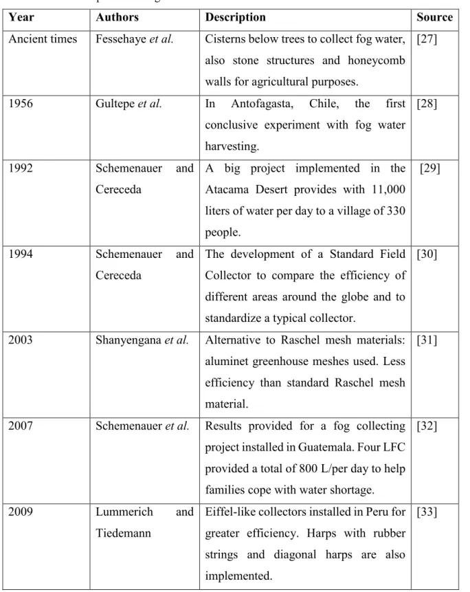
(17) cycloidal geometry for the collecting structure. A Quality Function Deployment (QFD) is presented in Annex A. Table 1. Time-line comparison of fog water harvesters.. Year. Authors. Description. Source. Ancient times. Fessehaye et al.. Cisterns below trees to collect fog water, [27] also stone structures and honeycomb walls for agricultural purposes.. 1956. Gultepe et al.. In. Antofagasta,. Chile,. the. first [28]. conclusive experiment with fog water harvesting. 1992. Schemenauer. and A big project implemented in the. Cereceda. [29]. Atacama Desert provides with 11,000 liters of water per day to a village of 330 people.. 1994. Schemenauer. and The development of a Standard Field [30]. Cereceda. Collector to compare the efficiency of different areas around the globe and to standardize a typical collector.. 2003. Shanyengana et al.. Alternative to Raschel mesh materials: [31] aluminet greenhouse meshes used. Less efficiency than standard Raschel mesh material.. 2007. Schemenauer et al.. Results provided for a fog collecting [32] project installed in Guatemala. Four LFC provided a total of 800 L/per day to help families cope with water shortage.. 2009. Lummerich. and Eiffel-like collectors installed in Peru for [33]. Tiedemann. greater efficiency. Harps with rubber strings and diagonal harps are also implemented. 17.

(18) 2010. Fessehaye et al.. SS mesh with polypropylene yarn.. [27]. 2010. Fessehaye et al.. 3D mesh structure with polymers.. [27]. 2014. Pinheiro et al.. VACNT´s with polyethylene generates a [13] hydrophobic-hydrophilic surface.. 2014. P. Moassam et al.. PDA-PP. make. a. hydrophobic- [12]. hydrophilic structure. 2014. Le Bouef and De la The results of a project to ensure a [34] Jara. freshwater source from fog collection. An average of 10 L/per m2/ per day was achieved. They highlight the feasibility of the project but mentions that more efficiency should be achieved.. 2017. Ye Tian et al.. Water collectors that mimic spider´s silk, [35] improved efficiency is reported.. 2018. Fessehaye et al. A 10 years project developed in Eritrea [36] which achieved 3.1 L per m2 per day. They highlighted the importance of seasonal fog collecting and the breaking of meshes.. 2018. Aliabadi et al.. Horn Lizard inspired fog collector.. [37]. 2018. Dai et al.. A hydrophobic directional rough surface [38] for a rapid nucleation and removal of droplets based on pitcher plants and rice leaves.. 2018. W. Shi et al.. Harp collector, using metallic materials [39] (aluminum and stainless steel), prevents clogging of water droplets and enhances efficiency of recollection.. 18.

(19) 1.2 State of the art To support this thesis, work of many papers was reviewed and analyzed, that are in the following resume (see the Table 1) [28–31]. The following analysis states solutions and important aspects for the design of different fog´s water collectors previously fabricated. 1.3 Biomimetic Biomimetic is used as inspiration to develop many models of fog collectors, the most recent research regarding this topic is presented in the inspiration taken from the Texas horned lizard [37]. Many different hydrophobic and hydrophilic profiles in a PMMA polymer were analyzed as well as different geometries of the meshes holes. They made a comparison between the different geometries and concluded that the collection rate is highly dependent of the geometry. The hydrophobic pattern has, generally, a better collection rate than the hydrophilic pattern in the polymer. Inspiration was taken from Stenocara gracilipes beetle´s profile. The super-hydrophobic surface generated by depositing polyethylene on pristine VACNT´s/steel screen and the super-hydrophilic surface by functionalized VACNT´s on carbon fiber. The collection result reported by the researchers had a best value of 30 L/m2∙h under controlled conditions [40]. The inspiration from cactus spines is implemented in 3D surface fog harvesting devices using also the dual profile hydrophilic and hydrophobic that has been reported before on dessert beetles [41]. A superhydrophilic-hydrophobic integrated conical stainless-steel needle is fabricated. The hydrophilic property is obtained by soaking it vertically in a dopamine solution, further painted with 3% chitosan solution followed by immersing vertically into a 5% glutaraldehyde solution and dried at vacuum. The super hydrophobic property was obtained by heating the needles at 200ºC and as they cooled down, they were covered by a 2% PVDF-HFP DMF solution. They reported an increase in water transportation due to the Laplace Force acting on the droplet and an efficiency of 235 mL after 200 minutes. Polydopamine (PDA) and negative photolithography method was used to produce a porous membrane with hydrophilic and hydrophobic patterns thanks to having a background of polypropylene (PP). This solution derives from the biomimicry of Stenocara gracilipes and the different profiles the insect carry on its back (hydrophilic bumps with hydrophobic surfaces). The efficiency reported is of 97 mg/cm2∙h[12]. 19.

(20) To prevent clogging formation of droplets that usually happens on normal mesh structures, “fog harps” were developed using different diameter string made of steel and aluminum in order to develop a fog harvesting device. The results provided by the researchers, state that they enhanced 3 times the efficiency of fog-harvesting rate compared to equivalent meshes [39]. 1.4 Background Science 1.4.1 Types of fogs Information regarding the types of fogs and their parameters taken from [42]. Precipitation fogs A type of fog that form during precipitation events, in these cases the air is colder than the falling raindrops. The wet-bulb temperature of a non-saturated air will be lower than the actual air temperature and that of the failing raindrops. This will cause evaporation of the raindrops to occur, a temperature drops from the air to its wet-bulb temperature and condensation. This often happens when two air masses with different properties interact together, so it is also known as “frontal fogs”. Other physical phenomena that may lead to precipitation fog formation are adiabatic cooling by orographic lifting, diabatic cooling, local-scale turbulent mixing of radiative cooling of nearsurface air over a wet land surface. This type of fog is recognized as a fog event if it is: •. Preceded by precipitation. •. Light rain or drizzle is present during fog duration with rates less than 14 mm/h.. Radiation fog This type of fog occurs often at night with a clear sky and calm winds. A radiative cooling phenomenon is present that causes the air to become saturated. Radiative cooling happens when the ground emits more long-wave radiation than it receives from the atmosphere. It can also be enhanced by sinking cold air into topographic depressions such as valleys and basins. Other factors that impact greatly the radiation fog formation are the moisture transport in the soil and the vegetation. This type of fog is recognized as a fog event if it has: •. Cloud cover less than 25% or cloudy with rise of cloud base before onset.. •. Wind speed less than 1.5 m/s. •. Cooling at onset or prior to onset with slight warming at onset. •. Onset between sunset and sunrise. 20.

(21) Advection fog This type of fog forms when warm air presents an advection phenomenon over a cold area. The air cools, saturates and forms a fog. They are formed, usually, over large water bodies with different surface temperatures and are expected to be frequent around islands, coastal areas, or inland-type areas near large lakes. That is the reason why it is also known as “sea fog”. This type of fog is defined as a fog event if: •. Wind speed is greater than 1.5 m/s. •. A sudden decrease in visibility is present.. Advection-radiation fog This type of fog derives from advection fog and forms when the advection phenomena takes place if sea are is transported via sea breeze over the land and is cooled during the night. They also form in coastal areas and have a limitation that is determined by how far inland the sea breeze front penetrates and remains through sunset. It is defined as a fog event if: •. Clear sky before fog onset. •. Onset during night-time. •. Slow visibility degradation before onset. •. Wind speed equal or greater than 1.5 m/s. Cloud base lowering (CBL) fog This type of fogs develops when the top of a stratus cloud acts as a radiative cooling surface and distributes the heat loss downward, cooling the air below the cloud layer and lowering the condensation level. For this fog to develops thin stratus clouds are usually required. It is defined as a fog event if: •. Cloud cover over 25%. •. Initial cloud height is 1 km. •. Gradual lowering of cloud base within 6 hours prior to fog onset.. Steam fog This type of fog may form over wet soil such as wetlands, swamps, rivers, lakes and irrigated croplands. Evaporation occurs from a warm water surface into cold air, leading to further 21.

(22) condensation. They often appear during calm wind conditions, however if the temperature difference is large enough, they can also form under strong wind conditions. The morning evaporation fog includes fogs that form 1 hour after sunrise. This type of fogs is heavily influenced by the presence of an artificial water body, since they are caused by the addition of moisture from these bodies to the air by evaporation. Steam fog, thus, needs and increase in specific humidity during fog formation regardless of the time of fog event (it does not matter if it occurs during morning-time or night-time). Steam fog is classified as a fog event if: •. The sky is clear before fog onset. •. There is an increase in the specific humidity of the air during fog onset.. 1.4.2 Condensation types and structure effects on condensation Condensation is an important phenomenon that directly affects the efficiency of water harvesting devices. The permeability of the surface (hydrophilic or hydrophobic), the nucleation energy and heat transfer coefficient are important factors that determine how water condensates. Water vapor has a reduced activation energy of heterogeneous nucleation compared to that of the homogeneous nucleation on a solid surface [43]. Two types of condensation are the ones that we are concerned with, primarily: dropwise and filmwise condensation. Filmwise In this type of condensation, the vapor condenses on thin layers of condensate already present. If the surface is hydrophilic, then condensation will be driven by the formation of an accumulative liquid film which is immobile. This means low heat transfer coefficient, despite the preference of the initial nucleation. Heterogeneous condensation occurs when vapor condenses on a cooled surface, when the surface is wettable, filmwise condensation occurs. [44], [45] Dropwise This condensation type is present when the surface is non-wettable, with an increase in heat and mass transfer performance, with easily removed condensed droplets. This means that dropwise condensation occurs on hydrophobic and superhydrophobic surfaces, it requires that the surface is continually bared to the vapor by the formation and coalescence of drops. The nucleation of drops. 22.

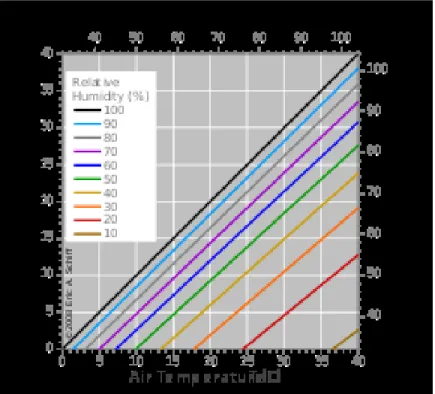
(23) is enhanced by the combination of small droplets, they get to form and reach a maximum size, before they drop due to the force of gravity[43,44]. 1.4.3 Temperature Effects on condensation Humidity is important in cloud and fog formation. Different temperatures have a great impact on the activation of the drop condensation nuclei. This nucleation requires supersaturation, more than 100% of relative humidity, in the direct vicinity of the particles. After activation of the nucleation phenomenon, condensation process decreases the gas phase humidity content, and increase the liquid water content, leading to a modification of the droplet size distribution. Adiabatic cooling, isobaric cooling and mixing of air flows with high relative humidity, but different temperatures, are some of the main processes leading to condensation. The point in temperature were the air starts to form drops is known as Dewpoint. In the following Figure 1 this is shown as a relationship of the air temperature and its relative humidity [46].. Figure 1. Relationship between air temperature, relative humidity and dewpoint.. 1.4.4 Cycloid To enhance the recollection efficiency, a geometry that follows the path of a cycloid is proposed. Since the cycloid resolves the problem of a curve that describes the fastest way a particle can reach 23.

(24) from point A to point B in the shortest amount of time, considering only the action of gravity, this kind of geometry should enhance the velocity of drop recollection. The equation used for the cycloid is solved as it follows: (Equation 1). If kinetic friction is included, the problem can also be solved analytically, although the solution is significantly messier. In that case, terms corresponding to the normal component of weight and the normal component of the acceleration (present because of path curvature) must be included. The tangent and normal vectors are: (Equation 2). gravity and friction are then: (Equation 3). and the components along the curve are: (Equation 4). so Newton's Second Law gives:. 24.

(25) (Equation 5). But: (Equation 6). So: (Equation 7). Using the Euler-Lagrange differential equation gives: (Equation 8). This can be reduced to: (Equation 9). Now letting: (Equation 10). the solution gives the following parametric equations: 25.

(26) (Equation 11). 1.4 Hypothesis and objectives Titanium dioxide and silver nanoparticles doped PCL matrix can be nano-structurally synthetized to improve water collection and purification rates that can be later used for the manufacture of weather conditions resistant and physiochemically balanced fog water harvesters. A novel geometry for the collector can be proposed via simulation and manufacturing methods to enhance water collection efficiency and mechanical properties to manufacture low-cost water harvesting devices. General objective: Develop a novel functional prototype of a fog´s water harvester validated trough simulation using a PCL polymer matrix doped with nanoparticles resistant to environmental conditions applied to commercial Rashel mesh that may improve collection´s efficiency of commercial Rashel mesh-based existing prototypes. Specific objectives: 1. Develop neat PCL, TiO2, Ag and Ag-TiO2 doped PCL membranes to obtain materials with hydrophilic and hydrophobic properties that improve commercial Raschel mesh performance in fog´s water collection. 2. Obtain the physical and chemical properties of the material. through the following. characterization techniques: TGA, DSC, XRD, SEM, TEM, FT-IR, HPLC, Contact angle, Roughness via Alicona, Uniaxial Test and Biaxial Test. 3. Development of a novel geometry trough computational simulation for the fog´s water collection device and manufacture a functional prototype that can be compared against collection efficiencies of existing models.. 26.

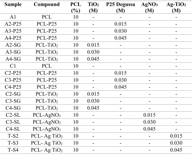
(27) CHAPTER 2 METHODOLOGY 2.1 Synthesis description and membrane preparation 2.1.1 Materials The reactive materials used to synthesize TiO2 and Ag-TiO2 for the membrane manufacturing are deionized water, nitric acid (95%) and titanium (IV) isopropoxide (97%), silver nitrate, PCL (Wm 80,000), chloroform, N,N-dimethyl-formamide (DMF) in a ratio of 97:3 (V:V) and acetic acid ( 95%), TiO2 and P25 Degussa, all of them purchased in Sigma Aldrich. All these materials were used without any further purification. 2.1.2 TiO2 synthesis by Sol-gel method The TiO2 NPs synthesis was carried out mixing deionized water, nitric acid (95%) and titanium (IV) butoxide (97%) in a 3-mouth flask at 25ºC under magnetic agitation. Subsequently, the solution was heated to 70-90 ºC for 8-12 hours and assisted with a water cooler reflux. The gel obtained was dried to 80ºC for 10 hours and thermally annealed at 400ºC for 4 hours to remove organic material, solvents and humidity. The procedure of the synthesis is detailed in [47]. 2.1.3 Ag-TiO2 synthesis by sol-gel method The synthesis was carried out mixing deionized water, nitric acid (Sigma Aldrich, 95%) and titanium (IV) isopropoxide (Sigma Aldrich, TTIP 97%) and Silver Nitrate (Sigma Aldrich) in a 3mouth flask at 25ºC under magnetic agitation. Subsequently, the solution was heated to 70-90 ºC for 4 hours and assisted with a water cooler reflux. The gel obtained was dried to 80ºC for 10 hours and thermally annealed at 400ºC for 4 hours to remove organic material, solvents and humidity. A one-hour hand-milling process was applied to homogenize the material obtained. 2.1.4 PCL composite membranes manufacturing The solutions used for the membranes production consisted in PCL pellets diluted in two solvents: chloroform with DMF in a ratio of 97:3 (V:V) and Acetic Acid (Sigma Aldrich) to obtain a 10 % 27.

(28) polymeric matrix solution. P25 Degussa, AgNO3 (Sigma Aldrich) and synthetized TiO2 and AgTiO2 were added in different concentrations 0.015 M, 0.030M and 0.045M into the polymeric matrix solution to obtain the doped ones. The solutions used for the membranes production are listed in Table 2. The polymeric solution was then deposited on glass substrate with further manual dispersion of the solution along the surface and then leave till solvent completely evaporates. Afterwards each membrane underwent a washing process which consisted of three cycles of 5 minutes each side under the water faucet and one minute of gentle shaking between each step. Table 2. Description of the solutions used to produce polymeric membranes. Sample. Compound. A1 A2-P25 A3-P25 A4-P25 A2-SG A3-SG A4-SG C1 C2-P25 C3-P25 C4-P25 C2-SG C3-SG C4-SG C2-SL C3-SL C4-SL T-S2 T-S3 T-S4. PCL PCL-P25 PCL-P25 PCL-P25 PCL-TiO2 PCL-TiO2 PCL-TiO2 PCL PCL-P25 PCL-P25 PCL-P25 PCL-TiO2 PCL-TiO2 PCL-TiO2 PCL-AgNO3 PCL-AgNO3 PCL-AgNO3 PCL- Ag TiO2 PCL- Ag TiO2 PCL- Ag TiO2. PCL (%) 10 10 10 10 10 10 10 10 10 10 10 10 10 10 10 10 10 10 10 10. TiO2 (M) 0.015 0.030 0.045 0.015 0.030 0.045 -. P25 Degussa (M) 0.015 0.030 0.045 0.015 0.030 0.045 -. AgNO3 (M) 0.015 0.030 0.045 -. Ag-TiO2 (M) 0.015 0.030 0.045. 2.2 Nanoparticles and developed membranes´ characterization 2.2.1 Thermogravimetric Analysis (TGA) Degradation Analysis The thermogravimetric analyses were performed on a TGA Perkin-Elmer Pyris 8000 equipment with a heating rate of 10°C/min. The samples were scanned in a temperature ranges from 50°C to 28.

(29) 600°C using nitrogen as purge gas and then heated up to 700°C in oxygen for ultimate thermooxidation. 2.2.2 Differential Scanning Calorimetry (DSC) Degree of crystallinity and melting temperature of PCL were measured by using a DSC PerkinElmer Pyris 8000 equipment. The melting temperature was determined considering the onset melting endotherm (𝑻𝒐𝒏𝒔𝒆𝒕 ). The degree of crystallinity (χc) was estimated using the enthalpy of 𝒎 melting change according to the equation: 𝜒𝑐=(𝛥𝐻𝑚)/(1−𝑤) ∆𝑯𝟎𝒎 , where 𝛥𝐻𝑚 and ∆𝑯𝟎𝒎 are the melting and the fully crystalline melting (139.5 J/g) enthalpies of the PCL, respectively, and w is the dopants weight fraction. All of the samples (average weight 10 mg) were held in standard aluminum pans and covers. The specimens were scanned from 50°C to 70°C with a heating rate of 10°C/min, in a nitrogen gas atmosphere. The DSC analysis curves for the material samples was carried out for the materials as received (first run data). 2.2.3 X-Ray Diffraction (XRD) The XRD measurements of developed composite membranes and bare materials were carried out using a PanAnalytical X'Pert Pro PW1800 diffractometer with a scanning rate of 2°/min and by using Cu–Kα radiation. The system was operated at 45 mA and 40 kV and the XRD data was collected in the 2θ range of 10º-40º. 2.2.4 Scanning Electron Microscopy (SEM) A SEM (ZEISS model EVO MA 25) was used with an accelerating voltage of 10.00 kV and a work distance of 7.0 mm to observe the morphology and state of aggregation of the samples in the form of powders and fibers of the synthesized compounds. 2.2.5 Transmission Electron Microscopy (TEM) A TEM (JEOL 2100) was used to observe the internal morphology of the clustered particles in order to determine the diameter of the synthetized TiO2 NPs. 2.2.6 Fourier Transformed Infrared (FT-IR) A FT-IR (Perkin-Elmer Frontier) equipment with an UATR accessory was used to carry out the IR analysis. The procedure consisted in placing the developed mesh scaffolds on the ZnSediamond crystal of the UATR and pressed with a tip to assure a good contact between the sample. 29.

(30) and the incident IR beam. The IR spectra were measured in the interval range of 4000 cm-1 to 380 cm-1 with a resolution of 4 cm-1, and by considering an average of 16 scans. 2.2.7 High-Performance Liquid Chromatography (HPLC) Analysis performed to determine the presence of Chloroform and Acetic Acid on the samples. This is done on the material with no dopants and the ones with the higher concentration of dopant. A base standard curve is first taken and then by duplicates each sample is measured. 2.2.8 Contact Angle (CA) CA measurements were performed using a Data physics (OCA, 15EC) system. The CA was measured between the mesh scaffold surface and a water droplet using SCA20_U software. The procedure consisted in placing a water droplet, from a dispenser with a volume capacity of 10 μL and deposition ratio of 2 μL/s, onto the mesh scaffold surface. The CA value retrieved from the calculation corresponds to the average considering the value calculated from the right and left side of the droplet. 2.2.9 Roughness properties measurement An Alicona (Infinite Focus microscope) was used to determine the roughness caused by the use of solvents during the manufacturing of the membranes. The parameters used to analyze the surface condition of the membranes were 700μs of brightness, 4 of contrast with an objective of 20X, VR of 0.60μm and LR of 6μm. The roughness average values were retrieved from the whole image area (1” X 1”). Compliance of ISO 4287 was achieved. 2.2.10 Uniaxial Mechanical Properties Uniaxial tests were performed using an Instron 3365 equipment, which can support loads between 5 N-5 kN. The calculations of the yield stress and ultimate tensile strength were retrieved considering a three-point average thickness according to the norm ISO-527-3 specimen type 4. 2.2.11 Biaxial Mechanical Properties Biaxial cyclic loading tests were performed using an ElectroForce LM1 TestBench. The major components of this system consist of four linear actuators and load cells attached to the end of the actuators, one in each direction. The maximum load allowed in the actuators is 17 N with a range of displacement of 19 mm. The strain field values on the sample surface were measured by using. 30.

(31) a digital image correlation (DIC) system Aramis V8. The measurements were performed at room temperature using a cruciform sample with geometry taken from [48], which consisted in a threecycle deformation with specified displacement of 1, 2 and 3 mm. In order to study the biaxial response caused by the loading and unloading cycles and the Mullins effect, the following expression proposed in [48], [49] is used to describe the stress-softening material behavior: (Equation 12). Here c is a constant parameter related to residual strains, b is a dimensionless material softening parameter, m represents the stretch intensity which is defined for equibiaxial extension as 𝒏 = √𝟐𝝀𝟐 + 𝝀−𝟖 , and mmax = M is the amount of maximum strain intensity at the point at which the material is unloaded, ℵ is a material response function [48] and λ represents the chain stretch. The corresponding principal engineering stress σ can be computed from the expression σ=TF-1 where F-1 represent the inverse of the tensor deformation gradient. 2.3 Membrane´s simulation 2.3.1 Air force calculation Smoke tunnel done with a speed of 2 m/s to observe the flux and the behavior or the air flow in two geometries: a half cycloid and a profile based on the Stenocara gracilipes beetle. For the simulation of forces acting on the mesh and obtaining the resultant force, the procedure form section 4.3.2.8 taken from Mexican Federal Electric Commission´s wind design manual [50] was used. This section corresponds to wind design for isolated signs and walls. To obtain the different constants required for the calculations, it was assumed that the structure would be functioning in Monterrey, Nuevo León; Mexico. Geometries were elaborated using SolidWorks software. The geometry profile for the curved surface is based in the cycloid curvature considering a friction coefficient μ = 0.30. Planar geometries were created considering a 10x10 cm surface area. 2.3.2 Software´s description Simulations performed using OpenFoam for the air flow simulation and ANSYS for the parts design and the simulation of the Finite Element Analysis (FEA). 31.

(32) 2.4 Prototype development 2.4.1 Film deposition on commercial Raschel Mesh Polymeric solution elaborated with PCL pellets, solvent and dopants were properly diluted in an Ultrasonic Tip. This solution was then sprayed over a HDPE commercial Raschel Mesh using an air painting gun from Surtek, with a pressure of 50 psi and at 10 cm from the mesh sample. Three layers of the solution were applied achieving a final thickness of 0.01mm. 2.4.2 Cross-linking After the application, the polymer underwent a cross-linking process of 3 hours. The set-up for the cross-linking is shown in Figure 22 and a long wavelength was employed for the UV radiation. The UV lamp is located at 15 cm from the center of the sample. 2.4.2 Pore geometry Pore geometry of the mesh is adapted from [51] using Type II of the explored geometries they proposed. The structure is trapezoidal and the geometry´s dimensions can be consulted in the annex. 2.4.3 Laser cut Laser cutting is performed in a Rayjet laser machine using the following parameters: speed 7.6 and power 50. 2.4.4 Efficiency test To be capable of obtaining the fog-harvesting efficiency value of the membranes that were sprayed with the selected polymeric solutions, laboratory-controlled conditions were set. The samples, along with a Sunbeam humidifier model 644 and a 4¨ fan from Steren were placed inside a squared crystal box with 50x50 cm dimensions. The relative humidity inside the collection´s chamber was set to 100%, temperature of the fog was 18.5ºC and a wind speed of 2.5 m/s. Different samples (10x10cm) were placed in the 3D printed frame and left for one hour. The water collected on a container was measured to obtain the values.. 32.

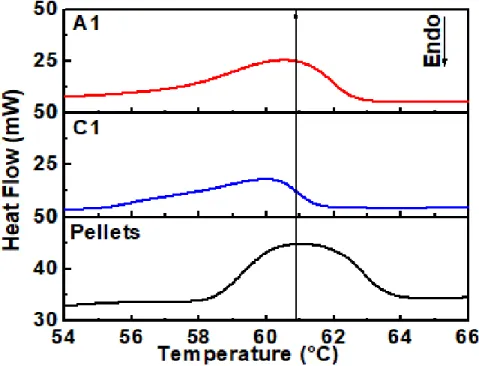
(33) CHAPTER 3 EXPERIMENTAL CHARACTERIZATION RESULTS AND DISCUSSIONS 3.1 Thermogravimetric Analysis (TGA) Degradation Analysis Thermal degradation analyses for PCL reference (pellets) and developed A1 and C1 composite membranes are shown in Figure 2. Temperature dependence of the PCL reference and samples A1 and C1 shows one-step weight loss between 360ºC-450ºC with an inflection point around 415ºC. Such thermal behavior is attributed, mainly, to the PCL decomposition to methyl pentanoate, water and carbon dioxide [52], [53].. Figure 2. Thermogravimetry Analysis of A1, C1 and Pellets Samples. And the derivate curves.. 3.2 Differential Scanning Calorimetry (DSC) As it was discussed previously, SEM analysis show a change on the surface morphology of the PCL membrane composites when using different solvents. In order to investigate the structural modifications in PCL caused by the solvents, DSC thermograms were measured for samples A1, 33.

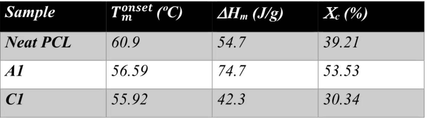
(34) C1 and compared with a PCL reference (pellet); the results are shown in Figure 3. The thermogram of the PCL reference (pellet) shows an onset melting temperature at 50.8ºC, as well as a broader melting curve between 58ºC and 64ºC. The thermogram for sample A1 (PCL membrane dissolved in acetic acid) shows a similar lineshape than PCL reference with a decrement of its amplitude and a increment of its broadening, such changes suggest that the acetic acid modifies in a low proportion the PCL crystal domains. On the other hand, the thermogram for sample C1 (PCL membrane dissolved in chloroform-DMF) shows that the lineshape has a shift to lower temperatures (below 60ºC) and the same broadening detected in sample A1.. Figure 3. Differential Scanning Calorimetry (DSC). The values calculated for 𝑻𝒐𝒏𝒔𝒆𝒕 , ∆𝑯𝟎𝒎 and χc are listed in Table 3. The χc value calculated for the 𝒎 PCL reference (39.2 %) is lower than the calculated for the sample A1 (53.6%), while the χc value for sample C1 (30.3%) is much lower than A1. The increment in the degree of crystallinity value in sample A1 is due to the broadening in its DSC lineshape. Contrary to A1, in sample C1 the decrement in its degree of crystallinity value indicates that the solvent had an impact in the formation of PCL crystal domains, as it was observed by DSC. SEM results in combination with. 34.

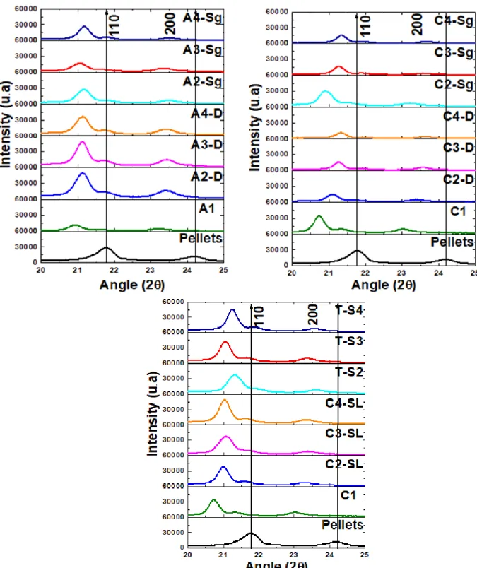
(35) DSC suggest that the chloroform-DMF promotes a better interaction with the PCL polymeric chains. Table 3. Comparison between offset melting temperature, change in enthalpy and percentage of crystallinity for Neta PCL, A1 and C1 samples.. Sample. 𝑻𝒐𝒏𝒔𝒆𝒕 (ºC) 𝒎. Hm (J/g). c (%). Neat PCL. 60.9. 54.7. 39.21. A1. 56.59. 74.7. 53.53. C1. 55.92. 42.3. 30.34. 3.4 X-Ray Diffraction (XRD) The diffractogram for the PCL reference (pellets) shows two peaks at 21.7º y 24.1º corresponding to (110) and (200) diffraction planes, as it is shown in Figure 4. These peaks are characteristic of the PCL orthorhombic unit cell [54]. As expected, the use of acetic acid as solvent [Figure 4 (a)] during the preparation of the PCL composite membrane (A1), induces a modification on the PCL crystal formation which is represented as a shift to lower angles of the (110) and (200) planes, as well as the detection of the (111) plane. The diffractograms for the rest of PCL-TiO2 composite membranes (A2-D, A3-D, A4-D, A2-Sg, A3-Sg and A4-Sg) show the same behavior that PCL reference membrane (A1), which indicate that the presence of TiO2 (P25 Degussa or the synthesized by sol-gel) does not modify the crystallization of the PCL matrix. Similar to A1, the PCL membrane manufactured using chloroform-DMF (C1) as a solvent [Fig. 4(b) and Fig 4(c).] induces a crystal modification and is represented as a shift to lower angles; and contrary to the manufactured ones using acetic acid, the diffractograms for PCL-TiO2 , PCL-Ag and PCL-Ag-TiO2 composite membranes using chloroform-DMF show different crystallizations, which are represented with a shift of the (110), (200) and (111) reflection planes. Such results are of great relevance, since corroborates the observations and analyses by SEM and DSC; and reveal that the presence of chloroform-DMF promotes the interaction of the different nanoparticles and the PCL polymeric chains thus, modifying in this way its crystallinity. 35.

(36) Figure 4. X-Ray Diffraction Analysis (XRD) for samples elaborated with synthetized TiO2, commercial TiO2 Degussa, Ag and Ag-TiO2 NP´s. Fig. 4a) samples elaborated with acetic acid. Fig 4b) samples. 36.

(37) elaborated with Chloroform-DMF. Fig. 4b) X-Ray Diffraction Analysis (XRD) for samples elaborated with synthetized TiO2 and commercial TiO2 Degussa. 3.5 Nanoparticles size (TEM) and Morphology of PCL membrane (SEM) When observing the TiO2 nanoparticles in the microscope, several clusters and agglomerations of the particles was detected (Figure 5). The size ranges from 150-300 nm in diameter. Afterwards, the images were analyzed via Transmission Electron Microscope. Figure 5 for the synthesized TiO2 NPs shows how the cluster observed in SEM is composed by isolated NPs with average sizes centered around 10 nm.. Figure 5. SEM image that shows a TiO2 cluster. TEM image that the TiO2 synthetized NP´s and their size.. The morphology obtained for the membrane composites are shown in the Figure 6 It is possible to note that the membranes manufactured with chloroform-DMF show a better surface homogeneity than the observed in the membranes manufactured with acetic acid, which exhibit porosity on the surface. Such behavior is attributed to a good nanoparticle dispersion and affinity between the reagents.. 37.

(38) C1. 20 m. C2-D. 20 m. 20 m A2-D. A1. 20 m. C2-Sg. 20 m. A2-Sg. 20 m. Figure 6. SEM morphology of PCL membranes with TiO2 nanoparticles.. Figure 7. SEM morphology of PCL membranes with Ag and Ag-TiO2 nanoparticles. Behavior of the polymer matrix regarding the dopant’s addition is similar when employing silver nanoparticles as can be observed in Fig.7. The use of chloroform as a solvent provides a good surface finish with low porosities. This only change whit the use of the Ag-TiO2 synthesis, which exhibits more porosities around the surface. Energy Dispersive Spectroscopy (EDS) was performed to show the presence of the desired elements inside the material. This confirms the realization of a composite material from the polymeric matrix and the nanoparticles.. 38.

(39) Figure 8. EDS diagram for A4-Sg membrane.. Figure 9. EDS diagram for C3-SL membrane.. Figure 10. EDS diagram for T-S3 membrane.. 39.

(40) 3.7 Fourier Transformed-Infra Red (FT-IR) The IR analyses of the developed composite membranes exhibit the characteristic vibrational modes of the PCL, as shown in Figure 11. The FT-IR spectrum measured for the PCL reference (pellet) shows modes at 2925 cm-1 and 2840 cm-1 corresponding to an asymmetric (νas) and symmetric (νs) stretching modes originated by CH=O groups, strong bands around 1725 cm-1 and 1698 cm-1 which are related to C=O stretching (νs) mode. The presence of CH2 and CH3 groups related to bending (δ) modes corresponding to the range 1473 cm-1 to 1342 cm-1 bonds respectively. Also, the regions of 1294 cm-1 and 1157 cm-1 are associated to the crystalline (νcr) and amorphous (νam) characteristics that corresponds to the C-O and C-C modes. On the other hand, the modes detected at 1240 cm-1 and 1170 cm-1 are associated to asymmetric (νas) and symmetric (νs) modes originated by COC groups. The FT-IR spectra of the developed composite membranes using acetic acid (Figure 11) shows the same vibrational modes than the reference, nevertheless in samples A1, A2-D, A3-D and A4-D the band for the C-O mode exhibit a shift to lower wavenumbers [55] due to the interaction between the solvent and TiO2 NPs, contrary to samples A2-Sg, A3-Sg and A4-Sg where the shift is not present. On the other hand, the spectra measured for the composite membranes developed using chloroform-DMF (Figure 11) shows the same shifts to lower wavenumbers thus indicating, as previously discussed, compatibility between the reagents, this includes samples elaborated with TiO2, Ag and Ag-TiO2.. 40.

(41) Figure 11. Fourier Transformed -Infra Red of all the samples compared against PCL Pellet. And detailed vibration bands for the functional C=O bond and the different dopants and solvents.. Interaction between the polymer matrix and the dopants is clearly observed when we zoom in to the shifts that vibration bands presents. This is observed in Fig 11. how the principal vibration bands shift as dopants are added, which presents and interaction and the confirmation of having a composite material. 3.8 High-Performance Liquid Chromatography (HPLC). 41.

(42) The test results obtained from HPLC for A1, when trying to identify traces of acetic acid inside the membrane are shown in Figure 12. Peak of the acetic acid presents an elusion at 9.108 minutes. It can be observed that for the A1 sample, no traces of solvent (up to 50 ppm) is present in the material. In the same way, for sample C1, with chloroform the result is shown in Figure 13. demonstrating that there is no peak present at 14 minutes in which chloroform presents its elusion.. Figure 12. Result for the HPLC performed on A1.. The sensibility of the chromatographer for sample A1 allows us to quantify values that exceed 50 ppm, in this case, since the peak is not visible, then our sample is below that the aforementioned value. The chromatographer for sample C1 has a higher sensibility, since the maximum permitted limit (MPL) is lower than 1 ppm. According to Mexican norms: NOM-199-SCFI-2017 and NOM250-SSAI-2014, that states the maximum values of acetic acid allowed for human consumption and the maximum values for chloroform in wastewater treatments, it can be concluded that sample A1 has an appropriate amount of solvent remnant for a secure use in the desired application. In the same way, as summed up in Table 4, chloroform was not detected when the material was characterized with the chromatographer. Both results validate the non-toxicity of the membrane and the safe use of them in water harvesting applications.. 42.

(43) Figure 13. Result for the HPLC performed on C1. Table 4. Maximum values (in ppm) allowed for chloroform and acetic acid in water and the results of the tests.. Solvent. Result (ppm). MPL (ppm). Acetic acid. Not detected. 1200. Chloroform. Not detected. 0.2. 3.9 Contact Angle The values for water contact angle are displayed in Figure 14. Reference samples A1 and C1 exhibit a similar hydrophobic permeability behavior due to the presence of CH2 groups in the PCL backbone. For composite membranes elaborated with acetic acid a relative decrement in the contact angle is observed (Figure 16), the latter could be associated to the low compatibility between the reagents as previously discussed. On the other hand, the samples developed with chloroform-DMF solvent exhibit slight changes on their water contact angle, while maintaining a hydrophobic behavior, compared to the reference, this can be attributed to the compatibility between the reagents. In specific, C3-Sg and C3-SL sample shows the best performance in water contact angle. 43.

(44) In the same way, the results obtained from uniaxial test measurements (Figure 14) show a lower mechanical performance for samples elaborated using acetic acid compared to those elaborated with chloroform-DMF solvent. Similarly, to contact angle results, sample C3-Sg presents better values in its mechanical properties. The difference in the yield stress values is due to the higher compatibility between the solvent used (chloroform-DMF) and the TiO2 and Ag NPs. Such results are in concordance with the results discussed in SEM morphology characterization and DSC.. Figure 14. Comparison between the contact angle and the yield stress for the different materials developed.. 3.10 Roughness test The images from the surface obtained with the Alicona microscope are shown in the following Figure number 15. In the image, the roughness of the sample A3-Sg and the different types of porosities can be appreciated. The difference of roughness between the composite membranes can be observed by analyzing the values obtained for each solvent, we observed that composite membranes using acetic acid presented higher roughness values [Figure 15], than that prepared with chloroform-DMF solvent [Figure 15]. As discussed previously, the decrement in the roughness values is attained to the compatibility between the reagents during the elaboration of composite membranes.. 44.

(45) Figure 15. Values of the roughness obtained via microscopy examination.. 3.11 Uniaxial mechanical properties Results of the mechanical tests are shown in the comparison graphics between contact angle and Yield stress. The results for the Ultimate Tensile Strength (UTS) of the sample tested is reported in the following Table 5 and show the same relationship and influence of the dopant on the samples. Table 5. UTS results comparison of the sample membranes.. Material A1 A2-P25 A3-P25 A4-P25 A2-Sg A3-Sg A4-Sg C1 C2-P25 C3-P25 C4-P25 C2-Sg C3-Sg. UTS (MPa) 2.35 1.90 2.45 2.6 3.19 2.78 2.14 6.03 7.29 13.93 15.03 11.67 15.47 45.

(46) C4-Sg C2-SL C3-SL C4-SL T-S2 T-S3 T-S4. 14.07 11.14 10.50 8.53 8.95 6.46 10.71. The information matches and shows how, mechanically, the sample C3-Sg exhibits good properties that are above from the rest of the samples tested. 3.12 Biaxial mechanical properties Figure 16 shows the performance of A1 and C1 material samples during the equibiaxial cyclic test. The data measured during the test are represented by black dots, while the solid lines are theoretical predictions computed from Equation (12). The material shear modulus µ, the chain number of links N, the energy density parameters A1 and A2, the stress softening and residual stress parameters b, and c used to fit experimental data in Equation (12) are summarized in Table 6. The sample C1, elaborated using chloroform-DMF as solvent, exhibit higher stiffness than the obtained for the sample A1 (elaborated with acetic acid as solvent), such values are 450 MPa and 130 MPa, respectively (Table 6). Table 6. Model parameters for equation fitting for both samples. Sample. µ (MPa). N. F. A1. A2. b. c. A1. 130. 4. 0.7. 0. -2700. 7. 2.5. C1. 450. 40. 0.6. 0. 0. 10. 15. 46.

(47) Figure 16. Results of the biaxial mechanical test performed on sample A1 and C1.. It can be noted that sample A1 absorbs less energy than sample C1 and has a greater elastic behavior and deformation value. The difference in engineering stress values, is in concordance with the rigidity values reported in Table 6 and the results obtained from uniaxial tests. The solvent has a great impact on the elasticity of the material, since the curves are barely shown for sample C1, it can be seen how the material has a very short elastic region compared to A1 which has a more elastic behavior. Additionally, there is a significant change in the energy absorption in both samples, A1 and C1, which is evident in the softening parameters b and c and in the permanent set values. As shown in Figure 16 and in Table 6, the sample C1 experiences almost no permanent set for this cyclic loading conditions.. 47.

(48) CHAPTER 4 COMPUTER MODELING OF THE OPTIMAL MESH GEOMETRY 4.1 Finite Element Analysis. Net pressure acting over the structure was calculated using the following equation: (Equation 13): 𝑝𝑛 = 𝐶𝑝𝑛 𝐾𝑝 𝑞𝑧. 𝑪𝒑𝒏 is the net pressure coefficient acting normal to the surface of the wall or sign, is obtained from Tables 4.3.16 (from (a) to (d)) and with the help of Figure 4.3.14 and Figure 4.3.15, dimensionless. 𝑲𝒑 the pressure reduction factor by porosity, dimensionless; this factor is given by: [1 - (1 - φ) 2], where φ is the solidity ratio of the sign or wall. φ ratio of the solid area between the total area of the sign surface or wall, dimensionless, and 𝒒𝒛 the dynamic pressure of the wind base calculated according to subsection 4.2.5, at height H of the sign or wall, in Pascals. The resulting pressure is calculated as: 𝑝𝑛 = (1.345)(0.684156)(58.21860575583594 𝑃𝑎 ) 𝑝𝑛 = 53.5721683511136375781308 𝑃𝑎. Thus, the resultant net force (𝑭𝒏 ) that the wind applies to the surface is the result of multiplying the net pressure times the area of application. In this case, the area selected (Areff) for the structural and geometrical analysis is equal to:. 48.

(49) 𝐴𝑟𝑒𝑓𝑓 = . 01𝑚2 𝐹𝑛 = .535721683511136375781308 𝑁. The mesh with the applied sample was cut using a laser machine, to perform the specified geometry pore sizes reported in [51]. This pore was selected due to its enhanced efficiency in drop collection. The pore was cut through the HDPE in the CAD design in order to compare the behavior of the air flow and the mechanical analysis and affectations that this pore will have on the meshes. HDPE was assumed has the dominant material in the mechanical behavior of the overall system.. Figure 17. Comparison between planar geometries with and without the pore geometry. Airflow and FEM analysis performed.. 49.

(50) Figure 18. Comparison between planar geometries with and without the pore geometry. Airflow and FEM analysis performed.. The graphical results shown from Figure 17 and 18 allows us to observe the behavior of the different geometries and how they deform when wind pressure is applied to them. The small values for the total displacements indicate that the HDPE meshes will not be affected by high wind pressures that may present at Monterrey city. None of the values exceeds or even get close to the yield strength of the polymer. However, there is no significative difference in the total deformation values that each of the solid experiments. Thus, indicating that the change in geometry and the pore cutting will not affect the mechanical stability of the membrane, making it a good candidate for being used as a fog-water harvesting device.. 4.2 Smoke tunnel and flow simulation for cycloidal geometry validation Two geometries were tested inside a smoke tunnel to compare the way the air flux passed around them in order to compare aerodynamic characteristics of both profiles, the smoke-flow is observed in Figure 19. One is based on the geometry of the Stenocara gracilipes beetle´s back and the other is an approximation to the beetles’ profile but assuming a half-cycloid. The path of the flow is 50.

(51) observed in the following figures and differences in the turbulence the flow presents at the end of the geometry can be clearly observed. Both geometries were tilted 27°, which test the collecting angle for a beetle similar to the Namib dessert beetle.. Figure 19. Geometry based on the Stenocara gracilipes beetle, tested in the smoke tunnel. Figure 22b) Halfcycloidal geometry tested in the smoke tunnel.. 4.3 Flow simulation over geometry profile. Afterwards, the complete cycloidal geometry was simulated in OpenFoam, to observe the flow behavior and how does it speed alongside the geometry profile and path. The following two images shows us the zone were the air speed increases, which goes in concordance with the proposed hypothesis and indicates the advantages in fog´s water collection and the efficiency increase.. Figure 20.. Simulation of the air speed changes whe10n passing over a cycloidal geometry. Figure 24b) Simulation of the air-flow stream lines that shows the increase in air speed alongside the geometry path.. Simulation shown in Figure 20 indicates us the red zone, located near the center of the geometry, which points the area where speed increases. Also, blue spots can be shown as locations where the air has less speed than the initial. These zones are also important, at the beginning and at the end 51.

(52) of the geometry, because they are important condensation points for a further speed increase in the drop leading to a higher recollection.. 52.