Astronomy
&
Astrophysics
https://doi.org/10.1051/0004-6361/201730562
© ESO 2018
Oxygen and zinc abundances in 417 Galactic bulge red giants
?
C. R. da Silveira
1, B. Barbuy
1, A. C. S. Friaça
1, V. Hill
2, M. Zoccali
3,4, M. Rafelski
5, O. A. Gonzalez
6,
D. Minniti
4,7, A. Renzini
8, and S. Ortolani
91Universidade de São Paulo, IAG, Rua do Matão 1226, Cidade Universitária, São Paulo 05508-900, Brazil e-mail:[email protected]
2Université de Sophia-Antipolis, Observatoire de la Côte d’Azur, CNRS UMR 6202, BP4229, 06304 Nice Cedex 4, France 3Pontificia Universidad Católica de Chile, Instituto de Astrofísica, Casilla 306, Santiago 22, Chile
4Millenium Institute of Astrophysics, Av. Vicuña Mackenna 4860, Macul, Santiago, Chile 5Space Telescope Science Institute, 3700 San Martin Drive, Baltimore, MD 21218, USA
6Institute for Astronomy, University of Edinburgh, Royal Observatory, Blackford Hill, Edinburgh EH9 3HJ, UK 7Departamento de Ciencias Físicas, Universidad Andres Bello, República 220, Santiago, Chile
8Osservatorio Astronomico di Padova, Vicolo dell’Osservatorio 5, 35122 Padova, Italy
9Università di Padova, Dipartimento di Astronomia, Vicolo dell’Osservatorio 2, 35122 Padova, Italy
Received 5 February 2017 / Accepted 21 February 2018
ABSTRACT
Context. Oxygen and zinc in the Galactic bulge are key elements for the understanding of the bulge chemical evolution. Oxygen-to-iron abundance ratios provide a most robust indicator of the star formation rate and chemical evolution of the bulge. Zinc is enhanced in metal-poor stars, behaving as anα-element, and its production may require nucleosynthesis in hypernovae. Most of the neutral gas at high redshift is in damped Lyman-alpha systems (DLAs), where Zn is also observed to behave as anα-element.
Aims. The aim of this work is the derivation of theα-element oxygen, together with nitrogen, and the iron-peak element zinc abun-dances in 417 bulge giants, from moderate resolution (R∼22 000) FLAMES-GIRAFFE spectra. For stars in common with a set of UVES spectra with higher resolution (R∼45 000), the data are intercompared. The results are compared with literature data and chemodynamical models.
Methods. We studied the spectra obtained for a large sample of red giant stars, chosen to be one magnitude above the horizontal branch, using FLAMES-GIRAFFE on the Very Large Telescope. We computed the O abundances using the forbidden [OI] 6300.3 Å and Zn abundances using the ZnI6362.34 Å lines. Stellar parameters for these stars were established in a previous work from our group.
Results. We present oxygen abundances for 358 stars, nitrogen abundances for 403 stars and zinc abundances were derived for 333 stars. Having oxygen abundances for this large sample adds information in particular at the moderate metallicities of −1.6 < [Fe/H] <−0.8. Zn behaves as anα-element, very similarly to O, Si, and Ca. It shows the same trend as a function of metallicity as theα-elements, i.e., a turnover around [Fe/H]∼ −0.6, and then decreasing with increasing metallicity. The results are compared with chemodynamical evolution models of O and Zn enrichment for a classical bulge. DLAs also show an enhanced zinc-to-iron ratio, suggesting they may be enriched by hypernovae.
Key words. Galaxy: bulge – Galaxy: abundances – stars: abundances
1. Introduction
Oxygen and zinc are key elements for the understanding of the star formation rate and chemical enrichment of the Galactic bulge. Oxygen is the prime and most robust probe for testing the timescale of bulge formation, because it has no contribution from SNIa, and because the prescriptions from different authors (e.g. Woosley & Weaver 1995, hereafter WW95; Kobayashi et al. 2006) produce the same behaviour.Woosley et al.(2002) describe the nucleosynthesis production of the different ele-ments. In all cases oxygen is produced in hydrostatic phases of massive star evolution.
?Observations collected at the European Southern Observatory,
Paranal, Chile (ESO programmes 71.B-0617A, 73.B0074A); TableB.1 is only available in electronic form at the CDS via anonymous ftp to http://cdsarc.u-strasbg.fr/ (130.79.128.5) or via http://cdsarc.u-strasbg.fr/viz-bin/qcat?J/A+A/vol/page.
Oxygen abundances in bulge field stars have been derived in several studies, among which the most recent are Alves-Brito et al. (2010); Bensby et al. (2013); Friaça & Barbuy (2017); Johnson et al. (2014); Jönsson et al. (2017); Meléndez et al. (2008);Rich et al.(2012); Ryde et al.(2010);Schultheis et al. (2017), andSiqueira-Mello et al.(2016). A review on abundances in the Galactic bulge is given in McWilliam (2016). A more general review on the MW bulge is presented inBarbuy et al. (2018).
[O/Fe] vs. [Fe/H] by the models, that occur when SNIa start to give a contribution in Fe.
Zinc is key to probe the contribution of hypernovae at the lower metallicities during the bulge chemical enrichment pro-cess. The high [Zn/Fe] ratios in bulge metal-poor stars can at present only be explained by enrichment from hypernovae (Kobayashi et al. 2006; Nomoto et al. 2013) as discussed in Barbuy et al.(2015). Zinc enhancements in metal-poor stars were derived in the literature also in halo stars byCayrel et al.(2004); Nissen & Schuster (2011), in the thick disk by Bensby et al. (2014);Reddy et al.(2006);Mishenina et al.(2011), and in metal-poor bulge stars byBensby et al.(2013,2017), andBarbuy et al. (2015).
Zinc is also useful for comparisons with data from damped Lyman-alpha systems (DLAs). DLAs are neutral hydrogen gas systems observed in absorption to background quasars, with minimum hydrogen column densities of 2×1020cm−2. DLAs dominate the neutral gas content at high redshift, and the metal-licity in DLAs is observed to decrease with increasing redshift (Pettini et al. 1999; Rafelski et al. 2012, 2014), similar to the decrease of metallicity with age of stars in our Galaxy. More-over, due to the neutrality of the gas, the metallicity of the gas can be measured quite precisely without ionization corrections, making them a premier site to measure abundances at high red-shift. Additionally, DLAs have been found to beα-enhanced and show enhanced [Zn/Fe] ratios (Rafelski et al. 2012).
We have previously studied the oxygen and zinc abundances in the Galactic bulge based on high resolution FLAMES-UVES spectra of 56 bulge giants (Zoccali et al. 2006; Lecureur et al. 2007;Barbuy et al. 2015; FB17). In the present work we derive O and Zn abundances for 417 red giants observed with FLAMES-GIRAFFE, within the same observational programmes as the FLAMES-UVES data, at the Very Large Telescope. The stars were observed in two fields, selected among the four fields observed by Zoccali et al.(2008): Baade’s Window (BW) (l= 1.14◦,b = −4.2◦), and a field at b = −6◦(l = 0.2◦,b = −6◦). These stars had already been analysed byZoccali et al.(2008), andGonzalez et al.(2011) derived abundances of theα-elements Mg, Si, Ca, and Ti for the sample.
The sample covers a range in metallicity [Fe/H] that allows us to investigate the bulge chemical evolution history in con-nection to other Galactic components. It includes 65 stars with [Fe/H]≤ −0.5, and 14 with [Fe/H]≤ −1.0, thus covering the required range, to help impose fundamental constraints on chem-ical enrichment models from oxygen and zinc abundances. This is so because the bulk of the bulge stars cover the metal-licity range of ∼−1.3 < [Fe/H] <∼+0.5 (Hill et al. 2011; Ness et al. 2013;Rojas-Arriagada et al. 2017;Zoccali et al. 2017), so that stars with metallicities in the range of−1.3 < [Fe/H] <−0.8 are important to understand the metal-poor end of the bulge chemical enrichment. A metal-poor end at these relatively high metallicities can be explained by the fast chemical enrichment that takes place in the bulge, rapidly reaching the metallicity of [Fe/H]∼ −1.0 (e.g.Cescutti et al. 2008, and in prep.; Wise et al. 2012). In other words, the equivalent of [Fe/H]∼ −3.0 in the halo, is [Fe/H]∼ −1.0 in the bulge. It can also help to bet-ter constrain the inbet-terfaces between the old bulge with the inner halo, and the thick disk. Hawkins et al. (2015) suggested that moderately metal-poor stars in the bulge could define the inter-face of Galactic disk and inner halo, by studying stars within
−1.20 < [Fe/H] <−0.55. The connection between thin and thick disks has also been studied byMikolaitis et al.(2014).
In the present paper we have adopted the chemodynami-cal evolution models for an old classichemodynami-cal bulge described in
Table 1.Fields observed: coordinates, distance to Galactic centre, red-dening as adopted inZoccali et al.(2008), number of stars observed, and typical signal-to-noise ratios.
Barbuy et al. (2015) and FB17, with some modifications. In Sect. 2 the observations are summarized. In Sect.2 the basic stellar parameters are reported, and the abundance derivation of O and Zn is described. In Sect.2 results and discussion are presented, including comparison with literature and chemody-namical evolution models. In Sect. 6 O-poor and N-rich field stars are selected. A summary is given in Sect.6.
2. Observations
The present data were obtained using the FLAMES-GIRAFFE instrument at the 8.2 m Kueyen of the Very Large Telescope, at the European Southern Observatory (ESO), in Paranal, Chile, as described in Zoccali et al. (2008; ESO Projects 071.B-067, 071.B-0014; PI: A. Renzini). Targets are bulge K giants, with magnitudes∼1.0 above the red clump, originally in four fields.
In the present work, we have analysed stars from two fields, reported in Table 1, among the four fields studied in Zoccali et al. (2008). These two fields were observed in setups HR13 (612.0–640.5 nm), HR14A (630.8–670.1 nm) and HR15 (660.7– 696.5 nm), with resolving power respectively ofR = 26 400, 18 000, and 21 350. The other two fields, NGC 6553 field at (l,b) = (5◦.25, 3◦.02) and Blanco field at (l,b) = (0◦,12◦), observed with setups HR11, HR13, and HR15, were reanalysed byJohnson et al.(2014), chosen by them because the HR11 setup contains copper lines. They derived abundances of the light elements Na, Al,α-elements O, Mg, Si and Ca, and the Fe-peak elements Cr, Fe, Co, Ni, and Cu, for 156 red giants in those fields.
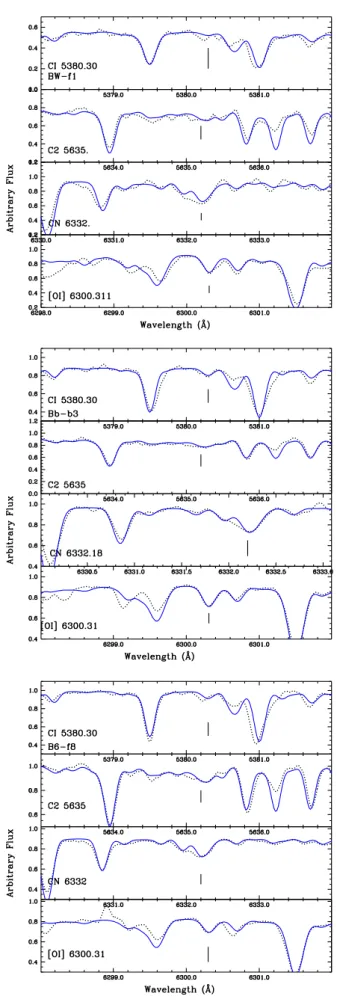
Given that the same stars observed with FLAMES-UVES were also observed with FLAMES-GIRAFFE, the oxygen and zinc were derived also from the GIRAFFE spectra. The fits to both UVES and GIRAFFE spectra are shown in Appendix A for the stars in common between the two.
stars identified by B6b, and faint ones by B6f. These iden-tifications for the UVES stars are inverted for the GIRAFFE identifications, that is, a BWb or B6b star in UVES will be a BWf or B6f in GIRAFFE, with numbers at random, corre-sponding to a random allocation of fibres for the observations with GIRAFFE.
3. Abundance analysis
Elemental abundances were obtained through line-by-line spec-trum synthesis calculations, carried out using the code described in Barbuy et al. (2003) and Coelho et al. (2005). The main molecular lines present in the region, namely the CN B2Σ−X2Σ blue system, CN A2Π−X2Σred system, C
2Swan A3Π−X3Π, MgH A3Π−X3Σ+, and TiO A3Φ−X3∆γand B3Π−X3∆γ’ systems were taken into account. The atmospheric models were obtained by interpolation in the grid of spherical and mildly CN-cycled ([C/Fe] = 0.13, [N/Fe] = +0.31) MARCS models by Gustafsson et al.(2008). These models consider [α/Fe] = +0.20. These models were chosen as these C and N abundances are compatible with the C, N values in normal red giants, and have suitableα-element enhancements.
We adopted the stellar parameters established by our group, given inZoccali et al.(2006,2008), and reported in TableB.1. A brief description of the methods follows:
– Photometric colours [V,I] were used together with colour-temperature calibrations by Ramírez & Meléndez (2005). Another useful indicator was also used: the intensity of TiO bands. Given that RGB stars were chosen, intentionally not very bright, in order to avoid too strong TiO bands, it was possible to define a TiO band index, measuring its strength at 6190–6250 Å, for stars withTeff <4500 K (seeZoccali
et al. 2008for further details). Effective temperatures were then checked by imposing excitation equilibrium for FeI and FeII lines of different excitation potential, using about 60 FeI lines, selected to be suitable for metallicities down to [Fe/H]∼ −0.8, and another line list for more metal-poor stars.
Since the final temperatures are spectroscopic, the red-dening E(B−V) and photometric temperatures were used only as initial guesses. The values of reddening reported in Table1are fromZoccali et al.(2006,2008), and are compat-ible with the minimum values given inSchlafly & Finkbeiner (2011) in fields of 2◦.1
– Photometric gravities of the sample stars were obtained adopting a classical relation, where the bolometric correc-tions were obtained using relacorrec-tions byAlonso et al.(1999). – Microturbulent velocitiesvtwere determined by imposing a
constant [Fe/H] derived from FeI lines of different expected equivalent widths.
– Finally, the metallicities for the sample stars were derived using a set of equivalent widths of FeIlines.
These stellar parameters were also adopted byGonzalez et al. (2011), for the derivation ofα-element abundances. For stars in common with the UVES data, the stellar parameters derived by Zoccali et al.(2006) from FLAMES-UVES data were used.
InZoccali et al.(2006) andLecureur et al.(2007), the oxy-gen abundance for the 56 giants observed with FLAMES-UVES were derived. InBarbuy et al.(2015) these values were revisited, with the unique aim of obtaining reliable CN strengths. In FB17 the oxygen abundances in stars of this sample, observed with both UVES and GIRAFFE spectrographs, were further revised 1 http://irsa.ipac.caltech.edu/applications/DUST/.
by taking into account in more detail the abundances of car-bon based on the C2(0,1) bandhead at 5635.2 Å and the CI 5380.3 Å line. These derivations replace the previous values by Zoccali et al. (2006), and Lecureur et al. (2007). A mean [C/Fe] =−0.07±0.09 was found for the UVES sample. Recently, Jönsson et al.(2017) and Schultheis et al.(2017) reanalysed a fraction of the FLAMES-UVES sample.
3.1. Zinc
InBarbuy et al.(2015), we derived zinc abundances for 56 red giants observed with the FLAMES-UVES spectrograph. The ZnI 4810.53 and 6362.34 Å lines were used to derive the zinc abundances. The sample in the present work contains 23 stars observed with UVES. We revised the Zn abundances from the ZnI 4810.53 Å line observed with UVES for stars in common with the present sample. The abundances from Barbuy et al. (2015) are reported in Table2. In a few cases a corrected value is indicated in bold face.
In the present work, the FLAMES-GIRAFFE spectra con-tain the ZnI 6362.34 Å line alone. As mentioned above, in AppendixAthe fits to this line with both UVES and GIRAFFE spectra are shown, for the stars common to the two samples. Lit-erature and adopted oscillator strengths were reported, together with blending lines in Table 1 ofBarbuy et al.(2015). The effect of a continuum lowering in the range∼6360.8–6363.1 Å, due to the CaI6361.940 autoionization line was taken into account. The continuum in the range 6361–6362 Å was the prime reference for fitting the Zn line, where the effects of the CaI autoioniza-tion line put this region and the ZnIline at the same continuum level. TheFWHMof lines was fitted for each star for a region around the ZnIline.
The ZnI 6362.339 Å line is sometimes blended with CN lines, as extensively discussed inBarbuy et al.(2015). For this reason, it is necessary to have a suitable derivation of C, N, and O abundances. In the present work we have derived Zn abun-dances for 333 stars among the 417 sample ones, where the line was well defined.
3.2. Carbon, nitrogen, and oxygen abundances
The derivation of C, N, and O abundances proceeded as described below.
Carbon: since the present spectra have neither the Swan C2 (0,1) A3Π−X3Π bandhead at 5635 Å, nor the CI 5380.3 Å line, and in the absence of a reliable C abundance indicator, we adopted a value of [C/Fe] =−0.2 for all stars, a deficiency expected in red giants (e.g.Smiljanic et al. 2009), compatible with the mean [C/Fe] = −0.07 found for the UVES sample, see FB17, their Table A.1. For stars that are also observed with UVES, as well as withZoccali et al.(2006);Barbuy et al.(2015), and FB17, the UVES results are preferred. The effect of C abun-dance in the O abunabun-dance is illustrated inBarbuy(1988, their Fig. 2). The N abundance, as derived from a CN bandhead depends on the C abundance adopted. Despite an uncertainty on the N abundance due to this assumption, we remind the reader that the main aim here is to be able to reproduce the CN line intensities, given the blend with CN lines on the right wing of the ZnI6362.339 Å line.
Tsuji 1973;Irwin 1988). In red giants N abundances are more informative on the CN-cycle than on chemical evolution. This is due to the transformation of C into N due to the CNO-cycle that takes place along the ascent of the giant branch. Added to the expected mixing process, there is an observed extra-mixing (see e.g.Smiljanic et al. 2009). Therefore the enhanced N abun-dances observed are due to stellar evolution processes, and do not reflect necessarily the N abundance of the gas from which the star formed. The very few cases of very high nitrogen abun-dances, combined with low oxygen abunabun-dances, are discussed in Sect.6.
Oxygen: the forbidden oxygen [OI]6300.311 Å line was used to derive O abundances, adopting log gf = −9.716, and tak-ing into account the blends with NiI lines at 6300.300 and 6300.350 Å, where we adopted Ni abundances varying in lock-step with Fe, as expected (e.g.Bensby et al. 2014,2017). A solar abundance ofA(O) = 8.76 is adopted (Steffen et al. 2015).
In conclusion, the abundances of N, O and Zn were derived iteratively in this order. The CN line intensity that appears as an asymmetry on the right wing of the ZnI6362 Å line, is also used to check the N and O abundances.
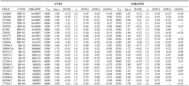
Table B.1 gives the atmospheric parameters adopted from Zoccali et al.(2008), and the resulting N, O, and Zn abundances for 417 stars in Baade’s window and the −6 degree fields. In Table2are presented the abundances derived for N, O, and Zn for the 23 sample stars having FLAMES-UVES spectra. The Zn abundances from the ZnI 4810 Å line were revised, and slightly modified in a few cases (indicated in bold face). For deriving the present N, O, and Zn abundances for these stars, we adopted the parameters from the UVES analysis (Zoccali et al. 2006; Lecureur et al. 2007). As explained above (Sect.3), the C, N, and O abundances reported first inZoccali et al.(2006) andLecureur et al.(2007), were partially revised inBarbuy et al.(2015), and the revision was further completed by FB17, and these latter are the values adopted here.
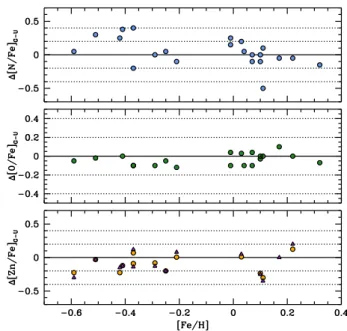
In Table3 we report the stellar parameters and N, O, and Zn abundances for the 23 stars from both UVES and GIRAFFE data. In Fig. 1 we compare the abundances of O, N, and Zn derived from the GIRAFFE data with those derived from the UVES spectra. The oxygen abundances are in very good agreement. Nitrogen abundances appear somewhat higher in GIRAFFE spectra with respect to those in UVES. For N we could not refit C, since we have no atomic or molecular line for this element, and this may be the source of the discrepancy. Zinc tends to be lower in GIRAFFE spectra than in the UVES ones; in Fig.1the difference is larger for the UVES values given for the mean of abundances derived from the two lines ZnI4810.5 and 6362.3 Å, and less discrepant when comparing results for the same line as in the GIRAFFE spectra.
3.3. Errors
For stars in common with UVES, we adopted the same uncer-tainties given in Barbuy et al. (2013), amounting to Teff ± 150 K for effective temperature, logg±0.20 for surface gravity, [Fe/H]±0.10 in metallicity, andvt ±0.10 km s−1 for microtur-bulent velocity. For the stars that have only GIRAFFE spectra we adopted higher uncertainties, due to having a lower reso-lution in the measurements of FeI and FeII lines, of±200 K forTeff,±0.40 for logg,±0.10 in [Fe/H] and±0.30 km s−1 for microturbulent velocity.
The errors in [O/Fe] and [Zn/Fe] are computed by using model atmospheres with parameters changed by these uncertain-ties, applied to the representative stars: the cooler star BW-b6,
Fig. 1.Comparison between GIRAFFE and UVES abundances for O, N, and Zn for the stars common to the two sets of spectra (Table3). For Zn: orange full circles consider the mean of two lines in the UVES results, and violet full triangles compare results for the same line.
and the hotter star B6-b3. Both of these were also analysed by Jönsson et al.(2017), as shown in Table5.
These uncertainties are given in Table 4. Since the stel-lar parameters are covariant, the sum of these errors is an upper limit. On the other hand, a continuum location uncer-tainty introduces a further unceruncer-tainty in [O/Fe]∼ ±0.05 and [Zn/Fe]∼ ±0.05.
4. Results
TableB.1reports the stellar parameters byZoccali et al.(2008) for the GIRAFFE sample. For stars for which we have both UVES and GIRAFFE spectra, the two sets of parameters and results are reported in Table B.1, with the UVES ones first, marked with a star (*), and the GIRAFFE ones just below. In this Table are given the OGLE, GIRAFFE and UVES names, stellar parameters, the derived N, O and Zn abundances, and theα-elements Mg, Si, Ca, and Ti analysed byGonzalez et al. (2011).
4.1. Oxygen abundances
In FB17 we discussed the available previous work on bulge sam-ples with reported derivations of oxygen abundances. These were the bulge dwarfs byBensby et al.(2013), the red giant stars from Alves-Brito et al.(2010) that were carried out in the optical for the same stars as in Meléndez et al. (2008); Cunha & Smith (2006); Ryde et al. (2010); Rich et al. (2012); Johnson et al. (2014);Rich and Origlia(2005) andFulbright et al.(2007).
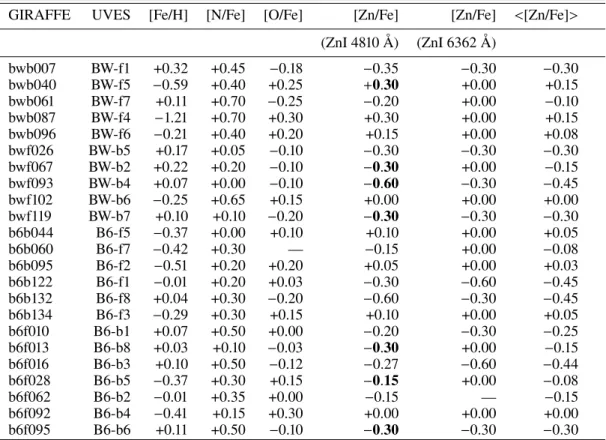
Table 2.Sample of stars observed with both FLAMES-UVES and FLAMES-GIRAFFE.
GIRAFFE UVES [Fe/H] [N/Fe] [O/Fe] [Zn/Fe] [Zn/Fe] <[Zn/Fe]> (ZnI 4810 Å) (ZnI 6362 Å)
bwb007 BW-f1 +0.32 +0.45 −0.18 −0.35 −0.30 −0.30
bwb040 BW-f5 −0.59 +0.40 +0.25 +0.30 +0.00 +0.15
bwb061 BW-f7 +0.11 +0.70 −0.25 −0.20 +0.00 −0.10
bwb087 BW-f4 −1.21 +0.70 +0.30 +0.30 +0.00 +0.15
bwb096 BW-f6 −0.21 +0.40 +0.20 +0.15 +0.00 +0.08
bwf026 BW-b5 +0.17 +0.05 −0.10 −0.30 −0.30 −0.30
bwf067 BW-b2 +0.22 +0.20 −0.10 −0.30 +0.00 −0.15
bwf093 BW-b4 +0.07 +0.00 −0.10 −0.60 −0.30 −0.45
bwf102 BW-b6 −0.25 +0.65 +0.15 +0.00 +0.00 +0.00
bwf119 BW-b7 +0.10 +0.10 −0.20 −0.30 −0.30 −0.30
b6b044 B6-f5 −0.37 +0.00 +0.10 +0.10 +0.00 +0.05
b6b060 B6-f7 −0.42 +0.30 — −0.15 +0.00 −0.08
b6b095 B6-f2 −0.51 +0.20 +0.20 +0.05 +0.00 +0.03
b6b122 B6-f1 −0.01 +0.20 +0.03 −0.30 −0.60 −0.45
b6b132 B6-f8 +0.04 +0.30 −0.20 −0.60 −0.30 −0.45
b6b134 B6-f3 −0.29 +0.30 +0.15 +0.10 +0.00 +0.05
b6f010 B6-b1 +0.07 +0.50 +0.00 −0.20 −0.30 −0.25
b6f013 B6-b8 +0.03 +0.10 −0.03 −0.30 +0.00 −0.15
b6f016 B6-b3 +0.10 +0.50 −0.12 −0.27 −0.60 −0.44
b6f028 B6-b5 −0.37 +0.30 +0.15 −0.15 +0.00 −0.08
b6f062 B6-b2 −0.01 +0.35 +0.00 −0.15 — −0.15
b6f092 B6-b4 −0.41 +0.15 +0.30 +0.00 +0.00 +0.00
b6f095 B6-b6 +0.11 +0.50 −0.10 −0.30 −0.30 −0.30
Notes.Metallicities [Fe/H] are fromZoccali et al.(2006), N, O abundances are fromFriaça & Barbuy(2017). [Zn/Fe] fromBarbuy et al.(2015) for ZnI4810.54 Å and if revised they are indicated in bold face; [Zn/Fe] for the ZnI6362.3 Å line in both UVES and GIRAFFE spectra are shown in AppendixA.
stars were given; (d) recent results for microlensed dwarf stars byBensby et al.(2017).
Figure3 shows the [O/Fe] vs. [Fe/H] for the present sam-ple (excluding six N-rich, O-poor stars), plotted together with oxygen abundances from UVES data for stars in common, anal-ysed both by FB17, and Jönsson et al.(2017), as well asRyde et al.(2010);Schultheis et al.(2017), andBensby et al.(2017). Also included are recent oxygen abundances for metal-poor stars located in outer bulge fields: five stars fromGarcía-Pérez et al. (2013), two stars fromHowes et al.(2016), and three stars from Lamb et al.(2017).
In Figs. 3 and 4 we overplot the behaviour of oxygen and zinc respectively, in chemodynamical models representing a classical bulge, as described in FB17, and briefly summa-rized as follows. The evolution of the model was followed up to 13 Gyr, and although the bulge is formed rapidly the star formation goes on, and the stellar mass is built up dur-ing at least ≈3 Gyr, allowing for a contribution from type Ia supernovae (SNIa). The best fit model for oxygen, based on previous data, was assumed to have a specific star formation rate ofνSF = 0.5 Gyr−1, following conclusions by FB17, and
Cavichia et al.(2014).
Comparison with literature. Part of the present data set has been under study recently byJönsson et al.(2017) andSchultheis et al. (2017). Given that this may be considered as a refer-ence sample for bulge studies, it is important to compare these different analyses.
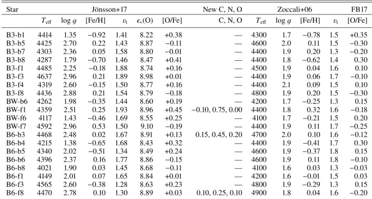
In Table 5 we give the stellar parameters rederived by Jönsson et al. (2017), their oxygen abundances given in
(O)2, and their [O/Fe] = (O)∗−(O)−[Fe/H], assuming (O) = 8.76 (Steffen et al. 2015). For a comparison with the present work, the stellar parameters fromZoccali et al. (2006) adopted in the present work and in FB17 are reported in the same table, and in the last column the abundance ratio of oxygen-to-iron as rederived by FB17.
We restrict these comparisons to the BW and−6◦ samples studied in the present work. For three stars (B6-b3, B6-f3, and B6-f8) the effective temperatures differ by ∆Teff (Zoccali+06-Jönsson+17) = −237 K, +364, and +232 K. For three stars the [O/Fe] value is different by more than 0.2 dex, with [O/Fe](Jönsson+17,FB17): BW-f1: +0.45,−0.18; B6-b3: +0.13,
−0.12; B6-f8: +0.03, −0.20, and we inspect these stars in particular more closely.
For these three metal-rich stars: BW-f1, B6-b3, and B6-f8, we employed the new stellar parameters from Jönsson et al. (2017), and rederived the C, N, and O abundances in the same way described in FB17, and the results are reported in Table 5. Only for BW-f1 the oxygen abundance differs from that of Jönsson et al., whereas for the other two stars they are simi-lar. Whereas the [O/Fe] values are comparable, it seems to us that both sets of parameters may be hinting at uncertainties: on the one hand, for some cases the gravities may be too high in Jönsson et al. given that we are dealing with stars located one magnitude above the horizontal branch, and on the other, the Zoccali et al. metallicities for some of the metal-rich stars may be too high. In the mean∆[Fe/H](Zoccali+06-Jönsson+17)
Table 3.Sample of 23 stars observed with both FLAMES-UVES, and FLAMES-GIRAFFE for comparison purposes.
UVES GIRAFFE
OGLE UVES GIRAFFE Teff logg [Fe/H] vt [N/Fe] [O/Fe] [Zn/Fe] Teff logg [Fe/H] vt [N/Fe] [O/Fe] [Zn/Fe]
433669 BW-f1 bwb007 4400 1.80 0.32 1.6 0.45 −0.18 −0.30 4300 1.67 0.32 1.5 0.30 −0.25 −0.40
240260 BW-f5 bwb040 4800 1.90 −0.59 1.3 0.40 0.25 0.00 5150 2.07 −0.59 1.4 0.45 0.20 0.30
357480 BW-f7 bwb061 4400 1.90 0.11 1.7 0.70 −0.25 −0.10 4800 2.06 0.11 1.4 0.20 −0.25 −0.15
537070 BW-f4 bwb087 4800 1.90 −1.21 1.7 0.70 0.30 0.15 5150 2.14 −1.21 1.1 0.54 0.30 —
392918 BW-f6 bwb096 4100 1.70 −0.21 1.5 0.40 0.20 0.08 4600 1.97 −0.21 1.4 0.30 0.08 0.22
82760 BW-b5 bwf026 4000 1.60 0.17 1.2 0.05 −0.10 −0.30 4300 1.87 0.17 1.5 0.00 0.00 —
214192 BW-b2 bwf067 4300 1.90 0.22 1.5 0.20 −0.10 −0.15 4450 1.96 0.22 1.3 0.15 −0.10 −0.20
545277 BW-b4 bwf093 4300 1.40 0.07 1.4 0.00 −0.10 −0.45 4100 1.84 0.07 1.2 −0.10 −0.20 —
392931 BW-b6 bwf102 4200 1.70 −0.25 1.3 0.65 0.15 0.00 4450 1.89 −0.25 1.5 0.70 0.10 0.20
554694 BW-b7 bwf119 4200 1.40 0.10 1.2 0.10 −0.20 −0.30 4300 1.89 0.10 1.2 0.10 −0.20 −0.10
33058c2 B6-f4 b6b044 4500 1.80 −0.37 1.4 0.00 0.10 0.05 4550 1.84 −0.37 1.7 0.40 0.00 0.08
100047c6 B6-f7 b6b060 4300 1.70 −0.42 1.6 0.30 0.25 −0.08 4350 1.72 −0.42 1.5 0.55 0.25 0.15
90337c7 B6-f2 b6b095 4700 1.70 −0.51 1.5 0.20 0.20 0.03 4850 2.02 −0.51 1.5 0.50 0.18 0.08
23017c3 B6-f1 b6b122 4200 1.60 −0.01 1.5 0.20 0.03 −0.45 4250 1.65 −0.01 1.5 0.35 0.07 0.00 11653c3 B6-f8 b6b132 4900 1.80 0.04 1.6 0.30 −0.20 −0.45 4850 1.91 0.04 1.5 0.35 −0.30 −0.50
21259c2 B6-f3 b6b134 4800 1.90 −0.29 1.3 0.30 0.15 0.05 5000 2.02 −0.29 1.5 0.30 0.05 0.13
29280c3 B6-b1 b6f010 4400 1.80 0.07 1.6 0.50 0.00 −0.25 4350 1.80 0.07 1.5 0.50 0.04 —
108051c7 B6-b8 b6f013 4100 1.60 0.03 1.3 0.10 −0.03 −0.15 4250 1.79 0.03 1.6 0.30 0.00 −0.05 31220c2 B6-b3 b6f016 4700 2.00 0.10 1.6 0.50 −0.12 −0.44 4400 1.81 0.10 1.7 0.40 −0.15 −0.05 31090c2 B6-b5 b6f028 4600 1.90 −0.37 1.8 0.30 0.15 −0.08 4700 1.98 −0.37 1.5 0.10 0.05 0.14 83500c6 B6-b2 b6f062 4200 1.50 −0.01 1.4 0.35 0.00 −0.15 4400 2.00 −0.01 1.4 0.60 −0.10 —
60208c7 B6-b4 b6f092 4400 1.90 −0.41 1.7 0.15 0.30 0.00 4400 1.83 −0.41 1.6 0.53 0.30 0.12
77743c7 B6-b6 b6f095 4600 1.90 0.11 1.8 0.50 −0.10 −0.30 4350 1.78 0.11 1.5 0.60 — −0.15
Table 4.Uncertainties on the derived [O/Fe] and [Zn/Fe] values for model changes of∆Teff = 150,200 K,∆logg = +0.2,0.4,∆vt = +0.1, 0.2, 0.3 km s−1, for UVES and GIRAFFE data respectively, and corresponding total error, applied to the stellar parametersT
eff, logg, [Fe/H],vtof stars BW-b6 (4200 K, 1.7,−0.25, 1.3 km s−1), and B6-b3 (4700 K, 2.0, 0.10, 1.6 km s−1).
Star Element ∆Teff ∆logg ∆vt (Px2)1/2 Continuum (Px2)1/2
(+150 K) (+0.2) (+0.1 km s−1) (parameters) (final)
UVES [C/Fe](CI) +0.00 +0.00 +0.00 +0.00 ±0.02 0.02
BW-b6 [C/Fe](CH) +0.00 +0.00 +0.00 +0.00 ±0.05 0.05
[N/Fe] −0.08 +0.02 +0.00 +0.08 ±0.02 0.08
[O/Fe] +0.00 +0.02 +0.00 +0.02 ±0.05 0.05
[Zn/Fe] −0.08 +0.06 +0.00 +0.10 ±0.05 0.11
∆Teff ∆logg ∆vt (Px2)1/2 Continuum (Px2)1/2
(+200 K) (+0.4) (+0.2 km s−1) (parameters) (final)
GIRAFFE [C/Fe](CI) +0.00 +0.00 +0.00 +0.00 ±0.05 0.05
BW-b6 [C/Fe](CH) +0.00 +0.00 +0.00 +0.00 ±0.05 0.05
[N/Fe] −0.10 +0.05 +0.00 +0.11 ±0.02 0.07
[O/Fe] +0.00 +0.05 +0.00 +0.05 ±0.05 0.07
[Zn/Fe] −0.10 +0.12 +0.00 +0.16 ±0.05 0.17
∆Teff ∆logg ∆vt (Px2)1/2 Continuum (Px2)1/2 (−150 K) (+0.2) (+0.1 km s−1) (parameters) (final)
UVES [C/Fe](CI) +0.08 +0.00 +0.00 +0.08 ±0.02 0.08
B6-b3 [C/Fe](CH) +0.00 +0.00 +0.00 +0.00 ±0.05 0.05
[N/Fe] +0.08 +0.00 +0.00 +0.08 ±0.02 0.08
[O/Fe] +0.00 +0.03 +0.00 +0.03 ±0.05 0.06
[Zn/Fe] −0.05 +0.03 +0.00 +0.06 ±0.05 0.08
∆Teff ∆logg ∆vt (Px2)1/2 Continuum (Px2)1/2 (−200 K) (+0.4) (+0.2 km s−1) (parameters) (final)
GIRAFFE [C/Fe](CI) +0.10 +0.00 +0.00 +0.10 ±0.05 0.11
B6-b3 [C/Fe](CH) +0.00 +0.00 +0.00 +0.00 ±0.05 0.05
[N/Fe] +0.10 +0.00 +0.00 +0.10 ±0.02 0.10
[O/Fe] +0.00 +0.05 +0.00 +0.05 ±0.05 0.07
[Zn/Fe] −0.07 +0.06 +0.00 +0.09 ±0.05 0.10
Notes.The errors are given such as the difference is the amount needed to recover the correct fit.
∼0.05dex. Except for a large difference in [O/Fe] for BW-f1, the two sets of results agree rather well, and are well-reproduced by the models.
Fig. 2. CNO abundances rederived for stars BW-f1 B6-b3, B6-f8, adopting stellar parameters defined byJönsson et al.(2017). Symbols: black dotted line: observed spectra; blue solid line: synthetic spectra.
These differences could be taken as the uncertainty expected from different analyses. The comparison of parameters results in the following differences: in effective tem-peratures ∆Teff (Jönsson+17-Zoccali+06) = −94 K, and
∆Teff(Schultheis+17-Zoccali+08) = +250 K; and in grav-ity values ∆log g(Jönsson+17-Zoccali+06) = +0.46 and
∆log g(Schultheis+17-Zoccali+08) = +0.10 (excluding the very discrepant star 2MASS 18042724-3001108). Schultheis et al.(2017) also found∆[Fe/H] (Schultheis+17-Zoccali+08) = 0.1 dex, and it is different if considering only the metal-poor and metal-rich stars separately where stars with [M/H] < 0 are systematically more metal-poor in Zoccali et al. (2008) with respect to the APOGEE measurements. The differences are larger in effective temperatures with respect to Schultheis et al. and in gravity with respect to Jönsson et al. (2017). The results will become more accurate in the near future, due to the possibility of fixing gravity values with data from the next release of theGaia Collaboration(2017).
4.2. Zinc abundances
Figure4 gives [Zn/Fe] vs. [Fe/H] for the sample stars, together with the UVES sample from Barbuy et al. (2015), the recent Zn abundances derived for 90 microlensed bulge dwarf stars by Bensby et al. (2017), and metal-poor stars analysed by Howes (2015); Howes et al. (2014, 2015, 2016) and Casey & Schlaufman(2015). This figure shows that for bulge metal-poor stars with [Fe/H].−1.4, Zn is enhanced with [Zn/Fe]∼+0.4. This behaviour is in agreement with the same trend of increas-ing [Zn/Fe] values with decreasincreas-ing metallicities for thick disk and halo stars as shown in Fig. 7 byBarbuy et al.(2015), where results byBensby et al.(2014);Ishigaki et al.(2013);Nissen & Schuster(2011);Mishenina et al.(2011);Prochaska et al.(2000); Reddy et al.(2006);Cayrel et al.(2004) were reported.
In Fig. 5, Zn abundances are plotted, compared with the α-element abundances of O, as derived in the present work, and Mg, Si, Ca, and Ti from Gonzalez et al. (2011). The trend shown by Zn appears similar to that of the α-elements, and more closely to oxygen, silicon, and calcium. The low [Zn/Fe] for high metallicity stars is compatible with the oxygen abundances.
Chemodynamical evolution models of zinc were com-puted for a small classical spheroid, with a baryonic mass of 2×10⁹ M
, and a dark halo mass MH = 1.3×10¹⁰ M, by Barbuy et al.(2015), FB17. The code allows for inflow and out-flow of gas, treated with hydrodynamical equations coupled with chemical evolution.
Table 5.Sample of stars observed with both FLAMES-UVES, and reanalysed byJönsson et al.(2017).
Star Jönsson+17 New C, N, O Zoccali+06 FB17
Teff logg [Fe/H] vt ∗(O) [O/Fe] C, N, O Teff logg [Fe/H] vt [O/Fe]
B3-b1 4414 1.35 −0.92 1.41 8.22 +0.38 — 4300 1.7 −0.78 1.5 +0.35
B3-b5 4425 2.70 0.22 1.43 8.87 −0.11 — 4600 2.0 0.11 1.5 −0.30
B3-b7 4303 2.36 0.05 1.58 8.80 −0.01 — 4400 1.9 0.20 1.3 −0.20
B3-b8 4287 1.79 −0.70 1.46 8.47 +0.41 — 4400 1.8 −0.62 1.4 0.30
B3-f1 4485 2.25 −0.18 1.88 8.74 +0.16 — 4500 1.9 0.04 1.6 0.10
B3-f3 4637 2.96 0.21 1.89 8.98 +0.01 — 4400 1.9 0.06 1.7 −0.10
B3-f4 4319 2.60 −0.15 1.50 8.77 +0.16 — 4400 2.1 0.09 1.5 0.10
B3-f8 4436 2.88 0.21 1.54 8.79 −0.18 — 4800 1.9 0.20 1.5 −0.30
BW-b6 4262 1.98 −0.35 1.44 8.60 +0.19 — 4200 1.7 −0.25 1.3 0.15
BW-f1 4359 2.51 0.25 1.93 8.96 +0.45 −0.10, 0.75, 0.00 4400 1.8 0.32 1.6 −0.18
BW-f6 4117 1.43 −0.46 1.69 8.55 +0.25 — 4100 1.7 −0.21 1.5 0.20
BW-f7 4592 2.96 0.53 1.50 9.10 −0.19 — 4400 1.9 0.11 1.7 −0.25
B6-b3 4468 2.48 0.02 1.67 8.91 +0.13 0.15, 0.45, 0.20 4700 2.0 0.10 1.6 −0.12
B6-b4 4215 1.38 −0.65 1.68 8.43 +0.32 — 4400 1.9 −0.41 1.7 0.30
B6-b5 4340 2.02 −0.51 1.34 8.49 +0.24 — 4600 1.9 −0.37 1.8 0.15
B6-b6 4396 2.37 0.16 1.77 8.86 −0.15 — 4600 1.9 0.11 1.8 −0.10
B6-b8 4021 1.90 0.03 1.45 8.68 −0.11 — 4100 1.6 0.03 1.3 −0.03
B6-f1 4149 2.01 0.07 1.65 8.84 +0.01 — 4200 1.6 −0.01 1.5 0.03
B6-f3 4565 2.60 −0.38 1.28 8.63 +0.23 — 4800 1.9 −0.29 1.3 0.15
B6-f8 4470 2.78 0.10 1.30 8.89 +0.03 0.10, 0.25, 0.10 4900 1.8 0.04 1.6 −0.20
Notes.Columns 8–11: stellar parameters fromZoccali et al.(2006); Column 12: [O/Fe] abundances fromFriaça & Barbuy(2017).
Fig. 4.[Zn/Fe] vs. [Fe/H] for the present sample (333 stars), compared with literature. Symbols: red filled circles: present work; black squares: results for stars in common based on UVES data (Barbuy et al. 2015); blue filled pentagons:Bensby et al.(2017); magenta open heptagons:Howes et al.(2015,2016); blue open heptagons:Casey & Schlaufman(2015). Chemodynamical evolution models by FB17 with formation timescale of 2 (black lines) and 3 Gyr (blue lines), or specific star formation rate of 0.5, 0.3 Gyr−1are overplotted. The model lines correspond to different radii from the Galactic centre: solid lines:r<0.5 kpc; dotted lines: 0.5<r<1 kpc; dashed lines: 1<r<2 kpc; long-dashed lines: 2<r<3 kpc. A typical error bar is indicated in the right upper corner, corresponding to a mean between the two reference stars (Table4).
range. It is important to note that chemodynamical models are suitable to indicate the inflexion of the [X/Fe] values due to enrichment of Fe from SNIa.
4.2.1. Comparison with literature
Comparisons with literature Zn abundances of microlensed dwarf bulge stars by Bensby et al. (2013), were discussed in Barbuy et al. (2015). In Fig. 4 we show the updated abun-dances for microlensed bulge dwarfs by Bensby et al. (2017). There is good agreement between the present results and Barbuy et al.(2015) and those by Bensby et al. at metallicities
−1.4 < [Fe/H] < 0.0, whereas the behaviour for metal-rich giants with [Fe/H] >0.0 are distinct. The microlensed dwarfs show a contant [Zn/Fe], whereas the bulge red giants show a decreasing trend with metallicity, although with a large spread of
−0.6 < [Zn/Fe] < +0.15.
At the high metallicity end, since there is progressive enrich-ment in Fe by SNIa, a constant [Zn/Fe] would imply that there is chemical enrichment in both Zn and Fe on similar timescales. Instead, a decrease of [Zn/Fe] would correspond to the enrichment in Fe by SNIa, with no enrichment in Zn by the same SNIa, as happens for theα-elements.
This discrepancy has been addressed byDuffau et al.(2017), who found, at supersolar metallicities, a decreasing [Zn/Fe] for red giants, and constant [Zn/Fe] for dwarfs. Their interpretation is that the dwarfs are old and the red giants are young. This inter-pretation cannot be applied here, given that at least part of the bulge metal-rich red giant stars should be old, as can be seen in
the distribution of ages given inBensby et al.(2017), see their Figs. 14 and 15).
The derivation of [Zn/Fe] in stars of dwarf galaxies by Skúladóttir et al.(2017;2018, and references therein) indicated a decreasing [Zn/Fe] with increasing metallicities. This behaviour is in agreement with an Fe enrichment by SNIa, but not with a Zn enrichment.
4.2.2. Comparison with damped Lyman-alpha systems
Fig. 5.[O, Mg, Si, Ca,Ti/Fe] vs. [Fe/H] and [Zn/Fe] vs. [Fe/H] for the 417 red giants. Symbols: Red filled circles: O from this work; Green filled circles: Zn from this work; Blue open triangles: Mg, Si, Ca, and Ti fromGonzalez et al.(2011). Typical error bars are indicated for [α/Fe] and [Zn/Fe].
rich regime, Fe is strongly depleted by dust, while on the metal-poor side, the oscillator strengths of Zn result in the absorption lines too weak to be detected in low-metallicity systems. To reduce the biases from dust depletion and undetected Zn absorp-tion lines, we limited our comparison in Fig.6to systems with
−2.5<[α/H]<−1.0. In this comparison, no correction for dust is applied.
Figure6a shows an enhanced zinc-to-iron ratio for the DLA data which is consistent with the present sample, although DLAs typically reside at lower metallicities. We note that Fig.6 exag-gerates the difference in metallicity ([Fe/H]) due to the removal of higher metallicity systems to avoid biases caused by dust depletion of Fe. Other literature data similarly show a spread in [Zn/Fe] (Akerman et al. 2005;Cooke et al. 2013– seeBarbuy et al. 2015), but is also compatible with a [Zn/Fe] enhancement. Cooke et al.(2015) argue instead that [Zn/Fe] in DLAs can be assumed to drop to solar at [Fe/H]≈ −2.0, based on a compi-lation of halo stars data by Saito et al. (2009). They assume therefore that Zn tracks Fe for [Fe/H] >−2.0. However, we show
in Fig.6a that both the present sample and the DLAs have ele-vated [Zn/Fe] at−2.5 <[α/H] <−1.0. Moreover, inRafelski et al.(2012), we find that Zn and S trace each other one-to-one, not consistent with the solar value, but rather consistent with the models inFenner et al.(2004), suggesting that Zn behaves like an α-element in DLAs, meaning that it is enhanced in metal-poor DLAs. In conclusion, Zn and α-elements show similar behaviour in metal-poor DLAs, and so can be expected to trace one another.
Fig. 6.Panel a:[Zn/Fe] vs. [Fe/H]: same as in Fig.4, including the damped Lyman-alpha systems data byRafelski et al.(2012). Models from FB17 are overplotted (same details as in Fig.4);panel b:[α/Fe] vs. [Fe/H]: data byRafelski et al.(2012), [O/Fe] in DLAs byCooke et al.(2015) and present results for [O/Fe] in the sample stars. The model lines inpanel a:correspond to the same Galactic bulge radii as in Fig.4. A typical error bar is indicated in the right upper corner in both panels: for [Zn/Fe] it corresponds to a mean value of the two reference stars given in Table4. For [α/Fe] the error is of±0.10 for both the stars and DLAs.
can be accomplished by studies of theα-enhancement [α/Fe] at [α/H].−1.0.
Figure 6b shows an α-element enhancement of DLAs at [Fe/H] <−1.0 compared with [O/Fe] values for the present sam-ple. In Fig. 6b we also include [O/Fe] values derived for metal-poor DLAs byCooke et al.(2015). The enhanced [α/Fe] for stellar data with [Fe/H] <∼−0.6, is consistent with the alpha-element enhancement of the DLA data.
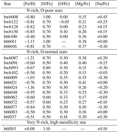
5. Oxygen-poor, nitrogen-rich stars
Enhanced nitrogen is expected in red giants due to CN-cycle (Iben 1967), and extra-mixing (e.g. Smiljanic et al. 2009, as reviewed byKarakas & Lattanzio 2014, and references therein). The situation is different for N-rich and O-poor stars, which were first detected in globular clusters (e.g. Sneden et al. 1997). These stars are not only O-poor and N-rich, but also
Na-rich, and anomalous also in Mg and Al. In the case of bulge red giants,Schiavon et al.(2017) identified N-rich stars, with a peak in metallicity at [Fe/H]∼ −1.0. They included in this category stars with [N/Fe]&+0.5, which in their sample of 5140 bulge giants, correspond to 58 of them, therefore in a proportion of 1.1%. Schiavon et al. interpreted these stars as second generation members evaporated from globular clusters. Carretta et al.(2009) have shown that second generation stars have low O, and high N and Na.
Table 6.N-rich and/or O-poor stars.
Star [Fe/H] [N/Fe] [O/Fe] [Mg/Fe] [Na/Fe] N-rich, O-poor stars
bwb008 −0.80 1.00 0.00 0.15 +0.45
bwb122 −0.81 0.70 −0.05 0.21 +0.25
bwb128 −0.82 0.70 0.00 0.23 +0.15
bwb130 −0.85 0.70 0.10 0.26 +0.15
b6b100 −0.40 0.50 0.00 0.36 +0.00
b6b011 −1.13 1.00 — 0.38 +0.00
b6b016 −0.81 0.70 — 0.37 −0.10
N-rich, O-normal stars
bwb087 −1.21 0.70 0.30 0.38 +0.20
bwb091 −0.60 0.50 0.40 0.40 −0.15
bwb093 −0.67 0.80 0.30 0.15 −0.30
bwb102 −0.50 0.50 0.20 0.15 −0.05
b6b009 −1.03 0.50 0.35 0.35 −0.30
b6b021 −0.76 0.70 0.30 0.41 +0.00
b6b024 −1.16 0.50 0.30 0.26 −0.20
b6b048 −0.95 0.50 0.33 0.25 −0.30
b6b062 −0.60 0.60 0.33 0.17 −0.05
b6b072 −0.57 0.60 0.25 0.27 +0.10
b6b077 −0.84 0.50 0.30 0.10 −0.30
b6b083 −0.50 0.50 0.30 0.18 +0.00
b6f037 −0.51 0.50 0.18 0.20 +0.30
Very N-rich, high metallicity star
b6f015 +0.08 1.10 — — +0.10
Notes.Na abundances are a mean of abundances from NaI6154.23 and 6160.75 Å lines.
with [Fe/H]≤ −0.5; (iii) one star very N-rich [N/Fe]>1.0 with [Fe/H] = +0.08 ([OI] line is blended with telluric lines in this case). These selected stars are listed in Table6, where besides the [Na/Fe] value reported, [Mg/Fe] values are also given for an indi-cation of theα-element enrichment in these stars as compared with the oxygen abundances.
If the criterion of [N/Fe]≥0.5 for stars with [Fe/H]≤ −0.5, is adopted, we find 21 stars, corresponding to about 5% of the sample. If we consider the N-rich ones together with [Na/Fe]>0.0, then we have 3.5% of them. Finally, if we dis-card the N-rich but O-normal, keeping only the O-poor ones ([O/Fe].0.1), then we have five stars left, corresponding to about 1% of the sample, in agreement with the percentage given by Schiavon et al. (2017). It would be interesting to derive Al for these stars in order to verify a possible Mg-Al anticorrelation also detected in second generation globular cluster stars. The cause of these anomalies is currently under debate in the literature, with the more massive low-Z asymp-totic giant branch stars as the likely site for such nucleosynthesis products (Renzini et al. 2015).
6. Summary
We studied oxygen and zinc abundances for 417 field red giants in the Galactic bulge. We were able to derive Zn, O, and N abun-dances for 333, 358 and 403 of them, respectively. We have identified five stars, corresponding to a 1% of stars that are simultaneously N-rich ([N/Fe]>0.5), and O-poor ([O/Fe].0.1), and this reduces to four stars if the more rigorous criterion of also being Na-rich ([Na/Fe]>0.0) is applied. According to
Schiavon et al.(2017), these characteristics could be attributed to evaporated second generation stars of globular clusters.
The sample contains a number of moderately metal-poor stars (−1.7 < [Fe/H] <−0.5) that define better the behaviour of [O/Fe] and [Zn/Fe] vs. [Fe/H] in this metallicity range. The present chemodynamical evolution modelling of a clas-sical bulge is able to reproduce the behaviour of O and Zn abundances in the Galactic bulge, except for Zn in the range
∼−1.6.[Fe/H].−0.8, where the yields from WW95 show a drop. We remind the reader that the models presented here con-sider yields from WW95 for [Fe/H]>−2.0, and a mean of mod-els by WW95 andKobayashi et al.(2006) for−4 < [Fe/H] <−2. The high [Zn/Fe] in very metal-poor stars favours enrich-ment from hypernovae, as defined byNomoto et al.(2013 and references therein) acting at these low metallicities. In damped Lyman-alpha systems (DLAs), a high [Zn/Fe] in metal-poor DLAs is also well reproduced by hypernovae yields. In DLAs Zn appears to behave similarly to α elements, and show an enhancement of [α/Fe] similar to the metal poor stars in the present sample. At the metal-rich end, a discrepancy persists between a decreasing [Zn/Fe] with increasing metallicity in the present sample of red giants, and an approximately constant [Zn/Fe] with metallicity for dwarf bulge stars. In conclusion, studies of the Galactic bulge with high-resolution spectroscopy for several hundred stars such as the present study, as well as work based on APOGEE data by Schiavon et al. (2017), and Schultheis et al. (2017), are crucial to better understand the chemical evolution and formation of the Galactic bulge.
Acknowledgements.CRS acknowledges a CAPES/PROEX PhD fellowship. BB
and AF acknowledge partial financial support by CNPq, CAPES and FAPESP. MZ and DM acknowledge support by the Ministry of Economy, Development, and Tourism’s Millenium Science Initiative through grant IC120009, awarded to The Millenium Institute of Astrophysics, MAS, and from the BASAL Center for Astrophysics and Associated Technologies PFB-06 and FONDECYT Projects 1130196 and 1150345. SO acknowledges the Italian Ministero dell’Università e della Ricerca Scientifica e Tecnologica (MURST), Italy.
References
Akerman, C. J., Ellison, S. L., Pettini, M., & Steidel, C. C. 2005,A&A, 440, 499 Alonso, A., Arribas, S., & Martínez-Roger, C. 1999,A&AS, 140, 261
Alves-Brito, A., Meléndez, J., Asplund, M., et al. 2010,A&A, 513, A35 Asplund, M., Grevesse, N., Sauval, A. J., & Scott, P. 2009,ARA&A, 47, 481 Barbuy, B. 1988,A&A, 191, 121
Barbuy, B., Perrin, M.-N., Katz, D., et al. 2003,A&A, 404, 661 Barbuy, B., Hill, V., Zoccali, M., et al. 2013,A&A, 559, A5 Barbuy, B., Friaça, A., da Silveira, C. R., et al. 2015,A&A, 580, A40
Barbuy, B., Chiappini, C., & Gerhard, O. 2018, ARA&A, submitted, [arXiv:1805.01142]
Bensby, T., Feltzing, S., & Lundström, I. 2004,A&A, 415, 155 Bensby, T., Yee, J. C., Feltzing, S., et al. 2013,A&A, 549, A147 Bensby, T., Feltzing, S., & Oey, M. S. 2014,A&A, 562, A71 Bensby, T., Feltzing, S., Gould, A., et al. 2017,A&A, 605, A89 Carpenter, J. M. 2001,AJ, 121, 2851
Carretta, E., Bragaglia, A., Gratton, R. G., et al. 2009,A&A, 505, 117 Casey, A. R, & Schlaufman, K. C. 2015,ApJ, 809, 110
Cavichia, O., Mollá, M., Costa, R. D. D., & Maciel, W. J. 2014,MNRAS, 437, 3688
Cayrel, R., Depagne, E., Spite, M., et al. 2004,A&A, 416, 1117
Cescutti, G., Matteucci, F., Lanfranchi, G. A., & McWilliam, A. 2008,A&A, 491, 401
Coelho, P., Barbuy, B., Meléndez, J., Schiavon, R. P., & Castilho, B. V. 2005, A&A, 443, 735
Cooke, R., Pettini, M., Jorgenson, R. A., et al., 2013,MNRAS, 431, 1625 Cooke, R. J., Pettini, M., & Jorgenson, R. A. 2015,ApJ, 800, 12 Cunha, K., & Smith, V. V. 2006,ApJ, 651, 491
Davis, S. P., & Phillips, J. G. 1963,The Red System (A2Π−X2Σ) of the CN molecule(Berkeley: University of California Press)
Fenner, Y., Prochaska, J. X., & Gibson, B. K 2004,ApJ, 606, 116 Friaça, A. C. S., & Barbuy, B. 2017,A&A, 598, A121
Fulbright, J. P., McWilliam, A., & Rich, R. M. 2007,ApJ, 661, 1152 Gaia Collaboration (Clementini, G., et al.) 2017,A&A, 605, A79 García-Pérez, A. E., Cunha, K., Shetrone, M., et al. 2013,ApJ, 767, L9 Gonzalez, O. A., Rejkuba, M., Zoccali, M., et al. 2011,A&A, 530, A54 Gustafsson, B., Edvardsson, B., Eriksson, K., et al. 2008,A&A, 486, 951 Hawkins, K., Jofré, P., Masseron, T., & Gilmore, G. 2015,MNRAS, 453, 758 Hill, V., Lecureur, A., Gómez, A., et al. 2011,A&A, 534, A80
Howes, L. M. 2015, PhD Thesis, Australian National University Howes, L. M., Asplund, M., Casey, A. R., et al. 2014,MNRAS, 445, 4241 Howes, L. M., Casey, A. R., Asplund, M., et al. 2015,Nature, 527, 484 Howes, L. M., Asplund, M., Keller, S. C., et al. 2016,MNRAS, 460, 884 Iben, I. Jr. 1967,ARA&A, 5, 571
Irwin, A. W. 1988,A&AS, 74, 145
Ishigaki, M. N., Aoki, W., & Chiba, M. 2013,ApJ, 771, 67
Johnson, C. I., Rich, R. M., Kobayashi, C., Kunder, A., & Koch, A. 2014,AJ, 148, 67
Jönsson, H., Ryde, N., Schultheis, M., & Zoccali, M. 2017,A&A, 600, A2 Karakas, A. I., & Lattanzio, J. C. 2014,PASA, 31, 30
Kobayashi, C., Umeda, H., Nomoto, K., Tominaga, N., & Ohkubo, T. 2006,ApJ, 643, 1145
Lamb, M., Venn, K., Andersen, D. et al. 2017,MNRAS, 465, 3536 Lecureur, A., Hill, V., Zoccali, M., Barbuy, B., et al. 2007,A&A, 465, 799 McWilliam, A. 2016,PASA, 33, 40
Meléndez, J., Asplund, M., Alves-Brito, A., et al. 2008,A&A, 484, L21 Mikolaitis, S., Hill, V., Recio-Blanco, A., et al. 2014,A&A, 572, A33
Mishenina, T. V., Gorbaneva, T. I., Basak, N. Y., et al. 2011,Astron. Rep. 55, 689 Momany, Y., Vandame, B., Zaggia, S., et al. 2001,A&A, 379, 436
Ness, M., Freeman, K., Athanassoula, E., et al. 2013,MNRAS, 430, 836 Nissen, P. E., & Schuster, W. J. 2011,A&A, 530, A15
Nomoto, K., Tominaga, N., Umeda, H., Kobayashi, C., & Maeda, K. 2006,Nucl. Phys. A, 777, 424
Nomoto, K., Kobayashi, C., & Tominaga, N. 2013,ARA&A, 51, 457 Pettini, M., Ellison, S. L., Steidel, C. C., & Bowen, D. V. 1999,ApJ, 510, 576 Prochaska, J. S., Naumov, S. O., Carney, B. W., McWilliam, A., & Wolfe, A. M.
2000,AJ, 120, 2513
Rafelski, M., Wolfe, A. M., Prochaska, J. X., et al. 2012,ApJ, 755, 89 Rafelski, M., Neeleman, M., Fumagalli, M., et al. 2014,ApJ, 782, L29 Ramírez, I., & Meléndez, J. 2005,ApJ, 626, 465
Reddy, B. E., Lambert, D. L., & Allende Prieto, C. 2006, MNRAS, 367, 1329
Renzini, A., D’Antona, F., Cassisi, S., et al. 2015,MNRAS, 454, 4197 Rich, R. M., & Origlia, L. 2005,ApJ, 634, 1293
Rich, R. M., Origlia, L., & Valenti, E. 2012,ApJ, 746, 59
Rojas-Arriagada, A., Recio-Blanco, A., de Laverny, P., et al. 2017,A&A, 601, A140
Ryde, N., Gustafsson, B., Edvardsson, B., et al. 2010,A&A, 509, A20 Saito, Y.-J., Takada-Hidai, M., Honda, S., & Takeda, Y. 2009,PASJ, 61, 549 Schiavon, R. P., Zamora, O., Carrera, R., et al. 2017,MNRAS, 465, 501 Schlafly, E. F., & Finkbeiner, D. P. 2011,ApJ, 737, 103
Schultheis, M., Rojas-Arriagada, A., García-Pérez, A. E., et al. 2017,A&A, 600, A14
Siqueira-Mello, C., Chiappini, C., Barbuy, B., et al. 2016,A&A, 593, A79 Skúladóttir, Á., Tolstoy, E., Salvadori, S., Hill, V., & Pettini, M. 2017,A&A, 606,
A71
Skúladóttir, Á., Salvadori, S., Pettini, M., Tolstoy, E., & Hill, V. 2018,A&A, in press, DOI:10.1051/0004-6361/201732359
Smiljanic, R., Gauderon, R., North, P., et al. 2009,A&A, 502, 267 Sneden, C., Kraft, R. P., Shetrone, M. D., et al. 1997,AJ, 114, 1964 Steffen, M., Prakapavicius, D., Caffau, E., et al. 2015,A&A, 583, A57 Tsuji, T. 1973,A&A, 23, 411
Udalski, A., Szymanski, M., Kubiak, M., et al. 2002,Acta Astron. 52, 217 Umeda, H., & Nomoto, K. 2002,ApJ, 565, 385
Umeda, H., & Nomoto, K. 2003,Nature, 422, 871 Umeda, H., & Nomoto, K. 2005,ApJ, 619, 427
Vladilo, G., Abate, C., Yin, J., Cescutti, G., & Matteucci, F. 2011,A&A, 530, A33
Wise, J. H., Turk, M. J., Norman, M. L., & Abel, T. 2012,ApJ, 745, 50 Woosley, S. E., & Weaver, T. A. 1995,ApJS, 101, 181
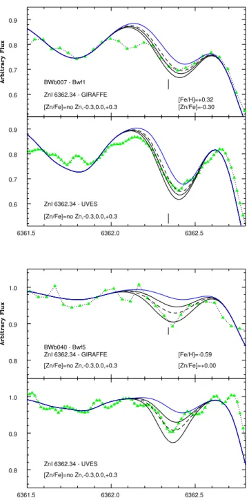
Appendix A: Comparison between GIRAFFE and UVES spectra
FiguresA.1present the fits of the ZnI 6362.3 Å line, for both spectra GIRAFFE and UVES for stars in common between the two sets of observations.
Fig. A.1.Comparison between UVES and Giraffe spectra with fits of the ZnI6362.3 Å line, for stars in common. Symbols: dotted black line and green filled triangles correspond to the observed spectra: black lines: synthetic spectra, dashed line: synthetic spectrum for the chosen [Zn/Fe] value. Blue solid line: synthetic spectra without Zn, showing the CN line.
Fig. A.1.continued.
Appendix B: Final abundances.
Table B.1.OGLE and GIRAFFE names, stellar parameters, resulting [N/Fe], [O/Fe], [Zn/Fe], and alpha-element abundances.
OGLE GIRAFFE Te f f logg [Fe/H] vt [N/Fe] [O/Fe] [Zn/Fe] [Mg/Fe] [Si/Fe] [Ca/Fe] [Ti/Fe]
Baade’s window bright: BW-f
423342 bwb002 4650 1.99 0.46 1.3 −0.05 −0.35 −0.30 −0.04 −0.08 0.13 0.03 423323 bwb003 4200 1.59 −0.48 1.5 0.00 0.10 0.22 0.43 0.26 0.15 0.23 412779 bwb004 4850 1.93 −0.37 1.5 0.20 — 0.13 0.23 0.22 0.29 0.48
412803 bwb005 4000 1.52 0.51 1.3 −0.20 −0.35 −0.40 — — — —
423359 bwb006 4650 1.92 −1.23 1.4 — — 0.30 0.34 0.43 0.30 0.48 433669* bwb007* 4400 1.80 0.32 1.6 0.45 −0.18 −0.30 −0.02 −0.10 0.01 −0.04 433669 bwb007 4300 1.67 0.32 1.5 0.30 −0.25 −0.40 −0.02 −0.10 0.01 −0.04 412752 bwb008 4900 1.98 −0.80 1.5 1.00 <0.00: — 0.15 0.30 0.34 0.51 412794 bwb009 4600 1.94 0.13 1.3 0.00 −0.25 0.00 −0.04 −0.08 0.28 0.30 402327 bwb011 4800 2.00 0.15 1.2 0.00 — −0.03 0.08 −0.17 0.36 0.20 412924 bwb014 4800 2.05 0.48 1.5 0.00 −0.40 −0.33 −0.04 −0.13 0.07 0.17 575317 bwb015 4550 1.78 0.22 1.4 −0.10 −0.35 −0.05 0.14 0.03 0.16 0.07 92600 bwb016 4250 1.70 0.05 1.0 0.50 −0.20 −0.05 0.20 0.08 0.15 0.29 412759 bwb017 4900 1.98 −0.39 1.4 0.30 0.30 0.20 0.24 0.16 0.26 0.31
575356 bwb021 4050 1.56 0.39 1.4 0.05 −0.30 — — — — —
423331 bwb022 4500 1.88 0.18 1.5 0.10 −0.30 −0.25 −0.02 −0.02 −0.06 −0.14 564797 bwb024 4200 1.69 0.24 1.5 −0.25 −0.30 — 0.02 −0.11 −0.01 0.08 564792 bwb025 5000 2.09 −0.68 1.4 0.00 <0.00: 0.10 0.28 0.30 0.32 0.36 412931 bwb026 4450 1.87 −0.15 1.3 0.20 0.04 0.05 0.25 0.11 0.25 0.31 564988 bwb027 4750 2.04 −0.24 1.4 0.30 0.15 0.30 0.32 0.14 0.19 0.43 412792 bwb030 4450 1.83 −0.26 1.4 0.10 — 0.12 0.29 0.18 0.20 0.43 564762 bwb031 4700 1.87 −0.63 1.6 0.25 0.30 0.15 0.35 0.36 0.19 0.49 564757 bwb033 4800 2.01 0.38 1.3 −0.25 −0.30 −0.15 0.04 −0.08 0.17 −0.07 564807 bwb035 4850 2.00 −0.67 1.5 0.30 0.35 0.15 0.34 0.32 0.26 0.34 575293 bwb037 4450 1.79 0.41 1.3 0.20 −0.25 0.00 0.09 −0.02 0.34 0.11 92537 bwb038 4500 1.81 −0.56 1.3 0.30 0.25 0.15 0.40 0.31 0.37 0.51 575303 bwb039 4850 2.02 −0.27 1.5 — — 0.10 0.35 0.26 −0.03 0.33 240260* bwb040* 4800 1.90 −0.59 1.3 0.40 0.25 0.00 0.29 0.09 0.27 0.35 240260 bwb040 5150 2.07 −0.59 1.4 0.45 0.20 0.30 0.29 0.09 0.27 0.35 82762 bwb041 4450 1.81 0.31 1.4 0.05 −0.30 −0.20 0.09 0.01 0.30 −0.06 92565 bwb042 4400 1.84 −0.05 1.5 0.40 — 0.15 0.06 0.01 0.06 0.16 240210 bwb043 4800 2.00 −0.04 1.2 0.30 0.00 0.00 0.23 0.22 0.31 0.28 554722 bwb044 4600 1.67 −0.44 1.6 0.40 0.10 — 0.20 0.26 0.12 0.36 82725 bwb045 4750 1.98 −0.70 1.3 — — 0.30 0.30 0.41 0.16 0.37 231262 bwb046 4930 2.04 −0.10 1.4 0.30 — — 0.16 0.10 0.07 0.30 231099 bwb047 5100 2.06 −0.22 1.6 0.30 −0.17 — 0.09 0.09 0.16 0.34 82747 bwb048 5000 2.06 −0.26 1.3 0.00 0.05 — 0.14 0.20 0.27 0.44 63856 bwb049 4700 2.01 0.33 1.3 0.00 −0.25 0.00 0.03 0.00 0.01 −0.06 231144 bwb050 4700 1.94 −0.20 1.5 0.45 0.05 0.10 0.24 0.01 0.22 0.47 231364 bwb053 4800 1.99 0.27 1.5 −0.10 −0.30 — 0.01 −0.11 0.10 0.04 82742 bwb054 4400 1.68 0.17 1.5 0.20 −0.30 −0.30 0.09 0.04 0.03 −0.11 73506 bwb055 4200 1.67 −0.24 1.5 0.50 0.10 — 0.30 0.09 0.10 0.29 222451 bwb056 4750 1.94 −0.33 1.3 −0.10 0.18 0.17 0.22 0.24 0.08 0.32 73504 bwb057 4550 1.92 −0.16 1.4 0.50 0.15 0.10 0.25 0.10 0.20 0.38 82761 bwb058 4800 2.01 −0.21 1.5 0.30 0.25 0.17 0.20 0.13 0.32 0.41 73490 bwb059 4300 1.74 0.49 1.2 −0.40 −0.35 −0.45 0.08 −0.04 0.04 0.00 222618 bwb060 4800 2.03 −0.33 1.4 0.30 0.15 0.10 0.28 0.17 0.31 0.44 357480* bwb061* 4400 1.90 0.11 1.7 0.70 −0.25 −0.10 −0.12 −0.10 0.08 0.00 357480 bwb061 4800 2.06 0.11 1.4 0.20 −0.25 −0.15 −0.12 −0.10 0.08 0.00 554664 bwb062 4600 1.91 −0.48 1.5 — 0.10 — 0.33 0.31 0.29 0.54 73514 bwb064 4900 2.04 −0.41 1.5 0.50 0.25 0.22 0.35 −0.04 0.29 0.50 205243 bwb065 4900 2.13 0.31 1.4 0.35 −0.30 0.00 0.16 −0.13 0.28 0.30 82705 bwb066 4500 1.80 −0.19 1.4 0.40 0.15 0.17 0.24 0.23 0.32 0.42 205257 bwb068 4600 1.94 −1.10 1.5 0.10 — 0.40 0.29 0.42 0.00 0.19
Table B.1.continued.
OGLE GIRAFFE Te f f logg [Fe/H] vt [N/Fe] [O/Fe] [Zn/Fe] [Mg/Fe] [Si/Fe] [Ca/Fe] [Ti/Fe]
82831 bwb069 4750 1.99 0.33 1.4 −0.05 −0.35 0.00 0.09 0.07 0.22 0.16 205436 bwb071 5200 2.27 0.16 1.4 0.30 −0.10 −0.20 0.05 −0.10 0.10 0.28 82798 bwb072 5050 2.17 −0.06 1.1 0.40 — 0.15 0.21 0.03 0.26 0.29 73515 bwb073 4550 1.81 −0.45 1.4 0.00 0.10 0.15 0.30 0.18 0.38 0.45 214035 bwb074 4650 1.92 0.26 1.4 0.25 — −0.30 0.08 −0.01 0.20 0.10 63794 bwb076 4750 2.00 −0.31 1.3 0.50 0.23 0.07 0.16 0.29 0.39 0.31 63792 bwb077 4450 1.82 −0.15 1.3 0.20 0.10 0.10 0.39 0.17 0.25 0.34 54167 bwb078 4800 2.06 −0.38 1.4 0.50 0.10 0.10 0.25 0.41 0.14 0.30 54104 bwb079 4550 1.95 −0.28 1.5 0.60 0.10 0.00 0.28 0.00 0.00 0.20 54132 bwb080 4950 2.06 −0.11 1.4 0.50 0.18 0.00 0.27 0.18 0.11 0.35
54273 bwb081 4850 2.12 0.45 1.3 0.20 −0.35 0.00 — — — —
44560 bwb082 4550 1.93 −0.23 1.4 0.20 0.13 0.00 0.14 0.12 0.16 0.21 205356 bwb083 4950 2.16 −0.19 1.5 0.65 0.15 0.10 0.11 0.17 0.01 0.01 63800 bwb085 4850 1.96 0.31 1.5 0.10 −0.40 −0.20 0.16 −0.14 0.25 0.12 63849 bwb086 4750 1.97 −0.92 1.4 0.30 0.30 0.15 0.35 0.41 0.33 0.48 537070* bwb087* 4800 1.90 −1.21 1.7 0.70 0.30 0.15 0.38 0.30 0.35 0.49 537070 bwb087 5150 2.14 −1.21 1.1 0.54 0.30 — 0.38 0.30 0.35 0.49 63823 bwb088 4550 1.87 −0.04 1.4 0.20 — 0.15 0.16 0.03 0.07 0.23 545401 bwb090 5150 2.22 0.01 1.4 — −0.10 −0.05 0.11 0.02 0.18 0.14 545440 bwb091 4500 1.91 −0.60 1.5 0.50 0.40 0.40 0.43 0.34 0.31 0.30 54311 bwb092 4900 2.15 0.26 1.5 −0.05 −0.30 0.00 0.06 −0.03 0.09 0.22 537101 bwb093 4800 2.07 −0.67 1.3 0.80 0.30 0.15 0.14 0.31 0.28 0.23 554655 bwb095 4900 2.03 −0.34 1.5 0.40 — 0.08 0.13 0.17 0.11 0.24 392918* bwb096* 4100 1.70 −0.21 1.5 0.40 0.20 0.08 0.11 0.10 0.24 0.32 392918 bwb096 4600 1.97 −0.21 1.4 0.30 0.08 0.22 0.11 0.10 0.24 0.32 63839 bwb097 4300 1.74 −0.22 1.4 0.30 0.20 0.10 0.24 0.09 0.21 0.25 554700 bwb098 4900 2.02 −0.17 1.4 0.20 — 0.05 0.11 0.15 0.14 0.31 554787 bwb099 4700 2.04 −0.58 1.2 0.00 0.15 0.18 0.31 0.31 0.39 0.36 63855 bwb100 4200 1.67 0.40 1.4 −0.45 −0.35 −0.40 0.14 0.10 −0.04 −0.04
63850 bwb101 4600 1.78 -1.61 1.6 0.00 0.35 0.40 — — — —
402294 bwb102 4800 2.05 −0.50 1.2 0.50 0.20 0.15 0.43 0.31 0.38 0.53 63820 bwb103 5100 2.19 −0.14 1.2 0.20 −0.10 0.08 0.11 0.10 0.31 0.27 393015 bwb104 4850 2.09 −0.06 1.3 0.20 0.02 0.02 0.41 0.02 0.36 0.35 554663 bwb105 4700 1.86 −0.72 1.3 0.40 0.35 0.22 0.40 0.44 0.36 0.33 63834 bwb106 4950 2.08 0.16 1.4 0.20 −0.30 −0.20 0.21 0.01 0.19 0.25 402361 bwb107 4950 2.00 −1.05 1.4 0.00 0.28 0.22 0.24 0.41 0.30 0.40 402307 bwb109 4600 1.93 0.40 1.5 −0.05 −0.40 −0.30 0.05 −0.11 0.17 0.10 402414 bwb110 4650 1.99 −0.21 1.4 0.20 −0.10 −0.20 0.39 0.29 0.11 0.49 545288 bwb111 4600 1.94 0.13 1.3 0.20 −0.30 −0.20 0.19 0.11 0.20 0.15 554889 bwb112 5000 2.18 −0.10 1.3 0.30 −0.10 −0.10 0.12 0.13 0.33 0.30 402315 bwb113 4750 1.97 −0.17 1.4 0.20 0.00 0.14 0.25 0.08 0.31 0.41 554811 bwb114 4900 2.11 0.17 1.3 0.15 −0.25 −0.15 0.04 0.00 0.30 0.05 234671 bwb115 4500 1.86 0.06 1.4 −0.15 −0.10 −0.10 0.04 −0.03 0.05 0.05 402332 bwb117 4500 1.82 −0.31 1.4 0.30 0.10 0.25 0.26 0.28 0.19 0.41 402322 bwb118 4800 1.94 −0.94 1.5 0.00 — 0.32 0.36 0.32 0.36 0.35 564743 bwb119 4250 1.70 0.21 1.4 0.20 −0.20 — 0.12 −0.04 0.03 0.06 402311 bwb120 4500 1.89 0.08 1.5 0.00 −0.20 0.10 0.12 0.00 0.15 0.26 244582 bwb122 4950 2.01 −0.81 1.3 0.70 <−0.05: 0.30 0.21 0.20 0.33 0.30 244504 bwb123 4550 1.83 −0.25 1.4 0.30 0.15 0.10 0.26 0.27 0.22 0.35 402607 bwb128 4800 2.04 −0.82 1.3 0.70 <0.00: 0.35 0.23 0.39 0.28 0.40 402531 bwb130 5100 2.21 −0.85 1.2 0.70 <0.10: 0.12 0.26 0.36 0.28 0.51 402325 bwb132 4500 1.87 −0.32 1.4 0.50 0.15 0.05 0.23 0.29 0.13 0.36
Table B.1.continued.
OGLE GIRAFFE Te f f logg [Fe/H] vt [N/Fe] [O/Fe] [Zn/Fe] [Mg/Fe] [Si/Fe] [Ca/Fe] [Ti/Fe]
Baade’s window faint: BW-f
585982 bwf003 4600 1.99 −0.08 1.4 0.20 −0.05 0.03 0.41 0.09 0.15 0.28 575308 bwf004 4350 1.84 0.27 1.4 0.10 −0.25 — 0.16 0.08 0.26 0.27 575289 bwf005 4450 1.92 −0.50 1.5 0.20 — — 0.49 0.21 0.29 0.45 423298 bwf007 4400 1.91 −0.08 1.2 0.50 −0.05 0.05 0.12 0.20 0.28 0.24 433830 bwf008 4200 1.87 0.18 1.5 0.20 −0.25 −0.25 0.25 −0.04 −0.08 0.00 564963 bwf009 4250 1.83 0.34 1.0 0.30 −0.30 −0.35 0.19 −0.05 0.14 0.14 554980 bwf010 4600 1.99 0.31 1.5 0.00 −0.40 −0.40 0.03 −0.18 0.03 0.08 423304 bwf013 4350 2.03 0.22 1.4 0.15 −0.30 −0.10 0.02 −0.09 0.06 0.24 102833 bwf014 4500 2.05 0.29 1.5 −0.10 −0.40 −0.15 0.11 −0.15 0.24 0.17 102853 bwf015 4400 1.86 0.15 1.2 0.45 −0.20 — 0.14 0.00 0.27 0.27 564768 bwf016 4150 1.74 −0.30 1.3 0.50 0.15 0.13 0.06 0.28 0.28 0.42 586077 bwf017 4500 2.02 0.21 1.3 −0.05 −0.30 −0.22 0.07 −0.16 0.04 0.08 586005 bwf018 4400 1.91 0.29 1.3 0.10 −0.30 — 0.00 −0.18 0.08 0.09 564789 bwf019 4100 1.70 −0.15 1.2 0.30 0.10 0.05 0.03 0.04 0.10 0.42 596502 bwf020 4150 1.87 0.28 1.1 0.35 −0.25 — 0.19 0.10 0.03 0.10
575360 bwf021 4500 1.96 −0.05 1.2 0.60 −0.10 — — — — —
Table B.1.continued.
OGLE GIRAFFE Te f f logg [Fe/H] vt [N/Fe] [O/Fe] [Zn/Fe] [Mg/Fe] [Si/Fe] [Ca/Fe] [Ti/Fe]
63840 bwf077 4500 1.99 0.31 1.1 0.15 −0.35 −0.60 0.15 −0.01 0.22 0.19 54108 bwf078 4400 1.91 0.46 1.5 −0.30 −0.30 −0.55 −0.09 −0.26 −0.02 0.03 54125 bwf079 4400 2.00 0.07 1.3 0.35 −0.15 — 0.18 0.22 0.19 0.28 73467 bwf080 4250 2.00 0.12 1.4 −0.30 −0.23 −0.20 0.08 −0.02 0.01 0.19
54133 bwf081 4050 1.67 0.35 1.0 −0.10 −0.33 −0.45 — — — —
54078 bwf082 4350 1.89 0.09 1.5 0.30 −0.20 −0.15 0.01 −0.01 0.26 0.08 63829 bwf083 4400 2.01 −0.01 1.5 0.80 −0.10 — 0.17 0.01 0.06 0.09 537095 bwf085 4500 1.93 0.31 1.2 0.00 −0.40 −0.40 0.05 0.00 0.17 0.04 545222 bwf086 4300 1.78 0.16 1.4 0.20 −0.20 −0.10 0.12 0.02 0.12 0.19 545438 bwf087 4350 1.97 0.12 1.5 0.30 −0.12 −0.15 0.16 −0.04 0.05 0.19 545233 bwf088 4350 1.88 0.31 1.3 −0.10 −0.35 — 0.07 −0.03 0.09 0.17 545313 bwf091 4400 2.05 0.16 1.4 −0.20 −0.13 −0.20 0.16 −0.05 −0.08 0.30 537092 bwf092 4600 2.03 −0.25 1.0 0.20 0.15 0.10 0.39 0.00 0.33 0.46
545277* bwf093* 4300 1.40 0.07 1.4 0.00 −0.10 −0.45 — — — —
545277 bwf093 4100 1.84 0.07 1.2 −0.10 −0.20 — — — — —
402415 bwf095 4600 2.08 0.01 1.2 0.10 −0.10 — 0.18 −0.05 0.00 0.31 554670 bwf096 4150 1.75 −0.26 1.3 0.35 0.13 0.25 0.25 0.26 0.18 0.48 554748 bwf097 4600 1.99 0.39 1.3 0.15 −0.40 — 0.07 −0.08 0.01 0.09 392952 bwf098 4200 1.79 0.13 1.5 0.40 −0.15 — 0.16 −0.14 0.12 0.09 392896 bwf099 4200 1.80 −0.12 1.3 0.70 0.15 0.05 0.20 0.16 0.06 0.38 393083 bwf100 4450 1.98 0.03 1.5 0.10 −0.05 0.00 0.19 −0.02 0.02 0.22 393053 bwf101 4250 1.83 0.49 1.2 −0.45 −0.38 −0.25 0.09 −0.15 0.04 0.03 392931* bwf102* 4200 1.70 −0.25 1.3 0.65 0.15 0.00 0.19 −0.03 0.03 0.09 392931 bwf102 4450 1.89 −0.25 1.5 0.70 0.10 0.20 0.19 −0.03 0.03 0.09 545269 bwf103 4250 1.83 0.45 1.1 −0.50 −0.35 — 0.09 −0.09 0.04 0.06 554683 bwf104 4500 2.00 −0.20 1.2 0.30 0.20 0.17 0.21 0.11 0.31 0.49 554668 bwf105 4300 1.85 0.08 1.3 0.30 −0.20 — 0.17 0.03 0.04 0.17 78106 bwf107 4300 1.98 −0.17 1.2 0.50 0.20 0.05 0.40 0.11 0.19 0.49 402498 bwf108 4450 1.90 0.55 1.2 −0.40 −0.40 — 0.06 −0.18 0.05 −0.05 234704 bwf109 4500 1.93 −0.18 1.4 0.10 0.20 0.17 0.26 0.09 0.21 0.36
67494 bwf110 4650 2.02 −0.05 1.1 −0.10 0.05 — — — — —
234701 bwf111 4500 1.98 0.12 1.2 0.45 −0.20 −0.05 0.24 −0.05 0.27 0.26 234888 bwf112 4200 1.94 0.28 1.5 −0.10 −0.35 — −0.60 −0.17 0.03 0.00 554713 bwf113 4250 1.90 0.20 1.4 0.20 −0.25 — 0.16 0.05 0.09 0.13 554956 bwf114 4600 1.99 −0.01 1.1 0.40 0.05 −0.12 0.19 0.03 0.30 0.49 392951 bwf115 4650 2.10 0.10 1.3 0.45 −0.30 — 0.11 −0.17 0.04 0.32 412750 bwf116 4350 1.83 0.11 1.1 0.25 −0.10 −0.05 0.14 −0.04 0.25 0.29 411479 bwf117 5200 2.32 −0.30 1.2 — 0.00 0.00 0.09 0.23 0.34 0.39 402656 bwf118 4750 2.08 −0.32 1.2 0.50 0.20 0.15 0.31 0.10 0.33 0.54 554694* bwf119* 4200 1.40 0.10 1.2 0.10 −0.20 −0.30 0.07 0.05 0.04 0.31 554694 bwf119 4300 1.89 0.10 1.2 0.10 −0.20 −0.10 0.07 0.05 0.04 0.31 402375 bwf120 4200 1.80 0.05 1.4 0.40 −0.15 — 0.22 0.02 0.20 0.25 244829 bwf121 4800 2.09 −1.09 1.4 0.30 0.23 0.35 0.43 0.47 0.36 0.50
402353 bwf122 4800 2.27 0.01 1.5 0.55 −0.15 — — — — —
Table B.1.continued.
OGLE GIRAFFE Te f f logg [Fe/H] vt [N/Fe] [O/Fe] [Zn/Fe] [Mg/Fe] [Si/Fe] [Ca/Fe] [Ti/Fe] Field at−6◦bright: B6-b
41958c3 b6b002 5100 2.04 0.05 1.5 0.45 −0.27 −0.32 0.20 −0.10 0.11 0.32
157820c3 b6b003 4800 1.87 −0.73 1.6 0.40 0.25 0.20 0.40 0.27 0.25 0.37
32799c3 b6b004 4850 2.04 −1.25 1.5 0.00 — 0.55 0.44 0.40 0.22 0.29
76187c3 b6b005 4550 1.79 −0.42 1.6 0.35 0.15 0.15 0.44 0.26 0.26 0.48
38354c3 b6b006 4700 1.83 −0.61 1.7 0.40 0.20 0.25 0.33 0.22 0.29 0.43
203158c3 b6b007 4800 1.86 −0.04 1.6 0.30 −0.12 0.05 0.29 0.01 0.09 0.38
39802c3 b6b008 5200 2.17 −0.50 1.6 — — 0.10 0.17 0.18 0.22 0.26
43054c3 b6b009 4800 2.01 −1.03 1.5 0.50 0.35 0.35 0.32 0.44 0.29 0.33
46885c3 b6b010 4350 1.70 0.00 1.5 0.50 0.00 0.04 0.15 0.10 0.17 0.04
1604c2 b6b011 4700 1.92 −1.13 1.4 1.00 — 0.45 0.38 0.46 0.39 0.47
36989c3 b6b012 4700 1.88 0.05 1.5 0.15 −0.23 −0.08 0.23 0.09 0.10 0.12
36067c3 b6b013 4550 1.78 0.08 1.4 0.25 −0.08 0.20 0.19 0.12 0.09 0.15
77454c2 b6b015 4950 1.95 −0.38 1.6 0.50 0.25 0.20 0.30 0.10 0.20 0.31
43562c2 b6b016 4600 1.84 −0.81 1.7 0.70 — 0.45 0.37 0.40 0.18 0.34
32832c2 b6b017 4350 1.71 −0.03 1.5 0.50 — — 0.17 −0.01 0.09 0.19
62009c2 b6b018 4350 1.73 −0.39 1.5 0.30 0.05 0.10 0.37 0.37 0.21 0.36
38565c2 b6b019 4600 1.87 −0.26 1.7 0.35 0.05 0.12 0.27 0.08 0.13 0.42
204270c3 b6b020 4900 2.05 0.02 1.3 0.10 −0.02 0.18 0.25 −0.02 0.28 0.20
69429c3 b6b021 4500 1.79 −0.76 1.5 0.70 0.30 — 0.41 0.39 0.24 0.36
56671c3 b6b022 4900 1.98 −0.20 1.3 0.30 0.05 0.17 0.24 0.11 0.30 0.14
25213c2 b6b023 4600 1.87 0.09 1.5 0.35 −0.15 −0.20 0.14 0.06 0.05 0.03
35428c2 b6b024 4800 1.92 −1.16 1.6 0.50 0.30 0.26 0.13 0.35 0.24 0.40
31338c2 b6b026 4700 1.89 −0.55 1.6 0.15 0.25 — 0.28 0.20 0.10 0.49
53477c2 b6b028 4650 1.85 −0.55 1.6 0.30 0.25 0.22 0.30 0.22 0.28 0.40
56410c2 b6b029 4600 1.81 −1.10 1.5 0.30 — 0.35 0.41 0.30 0.26 0.30
4799c2 b6b030 4950 2.10 −0.12 1.2 0.30 −0.15 0.05 0.26 0.26 0.41 0.42
43239c2 b6b031 5200 2.19 −1.26 1.6 0.00 — 0.28 0.31 0.30 0.20 0.46
14297c2 b6b033 4900 2.01 −0.66 1.8 0.40 0.30 0.30 0.51 0.29 0.11 0.41
17437c2 b6b034 4800 1.97 −0.50 1.6 0.70 0.25 0.33 0.39 0.25 0.29 0.53
41995c2 b6b035 4800 1.98 −1.58 2.0 — — — — — — —
30173c2 b6b036 4900 2.05 −0.90 1.7 0.40 — 0.38 0.21 0.38 0.23 0.44
45160c2 b6b037 4700 1.91 −0.56 1.5 0.40 0.28 0.20 0.41 0.09 0.32 0.47
13661c2 b6b038 4850 1.98 −0.09 1.5 0.30 −0.05 0.02 0.20 0.04 0.14 0.25
212324c6 b6b039 4800 1.88 −0.32 1.2 0.40 0.10 0.10 0.35 0.10 0.39 0.41
10381c2 b6b040 4700 1.90 −0.14 1.3 0.30 — 0.08 0.11 0.30 0.23 0.25
14893c2 b6b041 4050 1.51 −0.47 1.5 0.40 0.15 0.35 0.34 0.36 0.05 0.16
204828c2 b6b042 5000 2.10 −0.22 1.5 0.20 0.00 0.00 0.27 0.11 0.27 0.38
203913c2 b6b043 4900 1.93 −0.24 1.5 0.40 0.15 0.12 0.35 0.08 0.29 0.30
33058c2* b6b044* 4500 1.80 −0.37 1.4 0.00 0.10 0.05 0.41 0.09 0.26 0.40
33058c2 b6b044 4550 1.84 −0.37 1.7 0.40 0.00 0.08 0.41 0.09 0.26 0.40
212175c6 b6b045 4650 1.90 −0.47 1.5 0.40 0.27 0.08 0.38 0.26 0.33 0.55
213150c6 b6b046 4300 1.67 −0.02 1.5 0.25 −0.12 0.00 0.06 0.07 −0.04 0.16
1678c2 b6b048 4900 1.98 −0.95 1.8 0.50 0.33 0.25 −0.03 0.30 0.22 0.40
874c2 b6b049 4550 1.84 −0.32 1.5 0.60 0.20 0.17 0.32 0.00 0.24 0.42
7694c2 b6b050 5100 2.11 0.15 1.9 0.40 −0.35 −0.24 0.09 −0.04 0.06 0.19
8312c2 b6b051 5000 2.07 −0.32 2.0 0.40 −0.05 0.08 0.17 0.22 0.11 0.25
19402c1 b6b052 4550 1.83 −0.61 1.5 0.45 0.25 0.40 0.32 0.20 0.29 0.38
23483c1 b6b053 5150 2.01 −0.52 1.4 0.30 — 0.17 0.33 0.24 0.38 0.31
98692c6 b6b054 5000 2.22 0.07 1.4 0.30 −0.25 −0.32 0.17 −0.03 0.23 0.30
94324c6 b6b055 4700 1.90 −0.39 1.6 0.20 0.20 0.18 0.38 0.19 0.28 0.51
99147c5 b6b056 4550 1.86 −0.60 1.6 0.25 — 0.25 0.29 0.29 0.13 0.38
96158c6 b6b058 5000 2.10 −0.37 1.4 0.30 <−0.30: 0.15 0.35 0.16 0.31 0.54

![Fig. 4. [Zn/Fe] vs. [Fe/H] for the present sample (333 stars), compared with literature](https://thumb-us.123doks.com/thumbv2/123dok_es/3751291.643950/9.892.104.790.112.585/fig-zn-fe-present-sample-stars-compared-literature.webp)
![Fig. 6. Panel a: [Zn/Fe] vs. [Fe/H]: same as in Fig. 4, including the damped Lyman-alpha systems data by Rafelski et al](https://thumb-us.123doks.com/thumbv2/123dok_es/3751291.643950/11.892.101.790.123.776/fig-panel-including-damped-lyman-alpha-systems-rafelski.webp)