Multidimensional membership functions in T–S fuzzy models for modelling and identification of nonlinear multivariable systems using genetic algorithms

Multidimensional membership functions in T-S fuzzy models for

modelling and identification of nonlinear multivariable systems using

genetic algorithms

Jose Miguel Adanez Basil Mohammed Al-Hadithi Agustin Jimenez

A B S T R A C T

In this work, a new method for Takagi-Sugeno (T-S) fuzzy modelling based on multidimensional mem-bership functions (MDMFs) is proposed. It is verified that the fuzzy inference method of one-dimensional membership functions (lDMFs) may place the fuzzy rules in inappropriate locations for modelling of nonlinear multivariable systems, while the application of MDMFs allows a better identification through a smaller number of fuzzy rules. The proposed method uses a genetic algorithm (GA) for the adjustment of the MDMFs and the T-S method for modelling and identification of the nonlinear system. As a validation example, a nonlinear multivariable system, a coupled tanks system, is chosen. The results show that the proposed method presents less identification error than the T-S method, with less number of fuzzy rules.

1. Introduction

Fuzzy logic [1] has become an important technique for artificial intelligence, since the fuzzy logic allows to introduce the human uncertain behaviour to the computer definite performance. Fuzzy logic has become one of the most popular tools for modelling and control of nonlinear systems, especially the T-S fuzzy model [2], which allows the global identification of a nonlinear system as a set of linearized systems by fuzzy bending. Many works have been developed withT-S fuzzy models [3-5].

In [6], an approach developed by the authors is presented to improve the estimation of T-S models. The problem is that the original T-S identification method cannot be applied when the

triangular membership functions are overlapped by pairs. This restricts the use of this type of membership functions which have been widely used in the controllers design and are popular in in-dustrial applications. The approach, to search for an exact optimal solution, uses the minimum norm method although it increases complexity and computational cost. Another approach was devel-oped in [7], which can be considered as a generalized version of T-S method. This simple method with not much computational cost is based on weighting of parameters. In [8], this T-S identification method was extended to the multivariable case. These methods are characterized by the high accuracy obtained for modelling nonlinear systems in comparison with the original T-S method [2].

rules, but the generated rules can be placed in inappropriate loca-tions, which usually are not optimal and sometimes even do not correspond to the system data.

In order to solve this problem, the MDMFs [9] can be applied. The main idea is to generate the membership functions in the mul-tidimensional space, instead of generate lDMFs to be combined with fuzzy inference. These MDMFs can be located wherever the designer decides, but some algorithms have been developed to facilitate this task [10]. In [11], a clustering algorithm (fuzzy c-means [12]) is used for MDMFs location.

There are some variations of fuzzy clustering algorithms which obtain the fuzzy rules for the best separation of data in clus-tering problems. Some examples of this algorithms are fuzzy C-means [13-15], fuzzy possibilistics c-C-means [16], Gustafson-Kessel [17-19], Gath-Geva [20], and other approaches [21]. Instead of these clustering methods, our approach is based on the MDMFs location using a GA. An important advantage of the GA based proposed method with respect to deterministic clustering fuzzy approaches is that the proposed objective function for the GA is designed to find the MDMFs parameters which minimizes directly the T-S identification error.

The GAs [22,23] are optimization methods which use the prin-ciples of natural selection and genetics to find the optimal solution to a problem. The main advantage of the GAs is the inclusion of random changes in the solutions, which avoids that the algorithm falls in a local minimum permanently. As a main drawback, the GAs do not ensure the optimal solution in finite time, but with enough number of generations (the iterations of the GA), the GAs usually give good results with a reasonable computational cost. Several works present different applications of the GAs [24-26].

The GAs have been used with fuzzy based methods in some works [27-29]. The most prominent is the genetic fuzzy rule based system whose genetic process adjusts different components of a fuzzy system [30,31]. However, in our approach the GAs has been used for finding the best MDMFs location for a T-S identification. Once the MDMFs are successfully designed and the T-S identifica-tion is made, it is easy to create a fuzzy controller [32,33], which is out of the scope of this paper.

Summarizing, in this work it is verified that the fuzzy inference of lDMFs may place the fuzzy rules in inappropriate locations for modelling and control of nonlinear multivariable systems. Thus, in order to solve that, it is proposed the use of MDMFs which allows a better identification through a smaller number of fuzzy rules. A GA is proposed for the MDMFs automatic adjustment since this algorithm allows the convergence of the MDMFs parameters in a reasonable computing time. An illustrative example of a coupled tanks system is presented, which clearly shows the advantages of the proposed method.

The rest of this work is organized as follows. In Section , the T-S identification method based on lDMFs inference is de-scribed. In Section 3, the T-S model based on MDMFs is explained. The adjustment method for MDMFs based on GAs is presented in Section 4. In Section 5, an illustrative example of a coupled tanks system is presented to show the advantages of the proposed MDMFs adjusted by a GA over the traditional fuzzy inference of lDMFs

2. T-S identification method

The identification method of T-S fuzzy models is based on es-timating the nonlinear system parameters minimizing a quadratic performance index [2]. The traditional T-S identification method fails if the triangular membership functions of the fuzzy rules are overlapped by pairs, since the T-S matrix is not of full rank and thus it is not invertible [7]. Therefore, the authors in [7,8] proposed a generalized T-S identification, using a parameters weighting method.

The method is based on the identification of nonlinear functions which can be modelled as a set of difference equations by the following IF-THEN rules for an nth order system of s outputs and p inputs:

S( i l-i m ): If Z!(k) is Mj1 and . . . andzm(k) isMJ? then:

y{{k + 1) = a£"'i m ) + a[l,-'m)y,(k) + • • • + ^^y^k - n, + 1)

+ X ) b^-lm)uj(fc) H + ft^-^^jCfc - n, + 1)

(1) where {y-i(k),y2(k),.. .ys(k)} are the system outputs, {ui(k), u2{k),... up(k)} are the system inputs and {zi(fc), z2(fc),.. .zm(k)} are measurable variables, which hereinafter will be called fuzzy variables. In this fuzzy notation, j is the fuzzy variable index and i, is the fuzzy rule index associated with the fuzzy variable. The fuzzy estimation of the output becomes:

yj( k + l ) = ^ . . . ^ ^ ' "i m )( ^1. . .i m) ( f c ) ) M = l i m = l

p

+ b^''

u

(fc-n

+ l)] (2)

where

with fijdZj) being the membership function corresponding to the fuzzy set MJ. For the parameters weighting method, supposing

that a first affine linear estimation model is available. In other words, a first estimation of the following parameters is known: Po = [< . . . < b°n . . . b°lni ••• bg,i ••• b°m ]

In order to obtain this first estimation, the classical least squares method can be applied to the data set of the system. This estimation can be used as reference parameters for all the T-S fuzzy model subsystems

P o = [ Po Po ••• Po]'

rrr7-rm

Then, the fuzzy model parameters can be obtained minimizing

% n rm n

k=\ i , = l im= l j=0

= \\Y - XP\\2 + y2 \\p0 - P\\2

r

i

[_ KPo J

—

r x i

L

y l

\

where Y are the output data.X are the fuzzy input/output data and P are the parameters of the fuzzy model.

The y factor represents the degree of confidence of the parame-ters initially estimated [7,8]. Note that the matrixXa is of full rank, even if the triangular membership functions are overlapped by pairs. This solves the problem while the original T-S identification method fails. Thus the vector P can be computed as:

Incase if the state variables are measurable [8], Eq.

(1)

can also

be represented by a set of discrete state-space models as:

s(i,...im). I f z ^ i s Mh a n d a n d Z m(/<) i s Mkn t h e n.

x(k + 1) = a^-

+ A^-

x{k) + B

"

u(k)

Thus, the fuzzy identification can be made with state models [8]

using a similar formulation of Eqs.

(2)

and

(3).

Note that, in the T-S identification method, the fuzzy rules

weights u/

"

"

' = \XjL\ (l

jij(

j))

automatically generated by

lDMFs fijij(Zj) inference. The fuzzy rules generated by fuzzy

infer-ence, may not be suitable for optimal identification, even though

the lDMFs are well chosen, which is verified by an illustrative

example in Section

5.

In this work, the MDMFs are proposed to

solve this problem.

3. T-Sfuzzy model identification based on MDMFs

-2 -2

Fig. 1. Proposed MDMF.

The lDMFs fuzzy inference can generate some rules which are

not optimal for the fuzzy model, and even do not correspond

to the system data, which produces a loss of optimality and an

unnecessary computational cost.

MDMFs can be used to improve the model identification. Its

main advantage is that they are directly generated in the

multi-dimensional space. Some algorithms are used for automatic

ad-justment of MDMFs, such as clustering algorithms

[9,11].

MDMFs

can be designed with different shapes, for example n-dimensional

pyramids

[10].

Our approach with multidimensional fuzzy sets M

is as follows.

The fuzzy variable is defined as:

Z = [ Z\ 7-2

z e 9i

* r

and the MDMF ^(z).

For each fuzzy set M\ a central point z

e W is defined and for

eachz(k) e $, a quadratic distance is defined as:

(6)

d, (z(/<)) = Ej=i P« (zj(k) - z

)

> o

where p

e W is a design parameter vector which weights the

distances.

The MDMF

(Fig. 1)

is:

1

IM (Z('<)) (7)

1 + d, (z(/<))

which has the advantage of being 1 for the central point and

between 0 and 1 for the rest of the space. The function decreases

as the points move away from the central point. In addition, the

function is derivable with respect to any parameter.

This approach can be considered as an approximation of a

Gaussian radial-basis function with less computational cost. This

is important because the same fuzzy rules designed for modelling

and identification stages must also be applied at control stage,

which is online and therefore, the computing time becomes crucial.

The T-S fuzzy model of the system with n

rules is:

S'lIfzMisM'then:

yi(k + 1) = a\

+ a'

yi(k) + • • • + a'

yi(k - m + 1)

p

+ J2

\n

W + ••• +

\m

i('< - "l + 1) (8)

And the system becomes:

yi(k +\) = Y^on (z(k)) [a\

+ a'

yi(k) + • • •

i = l

+ a'

y

(k-n

+ l)

p

+ J2

w

W + ••• + b^ujik -

+1)]

where

, ,M, Mi(z(k))

Qfj (Z(fc)) = ^ ^

(9)

(10)

4. MDMFs design based on GA

In the previous section the MDMF functions

(7)

are defined,

but the MDMFs parameters (z

and p

) must be calculated for an

optimal T-S identification. In order to obtain the MDMFs

parame-ters (antecedents) and the T-S model parameparame-ters (consequents),

several methods applying different adjustment algorithms have

been assayed.

The first algorithm is based on the optimal adjustment of

MDMFs through a variation of an algorithm developed by the

authors in

[34,35].

The algorithm performs a recursive adjustment

of the T-S antecedents through an extended Kalman filter

[36].

Unfortunately, with this method, the antecedents convergence is

not guaranteed. A second method consists on applying an

opti-mization algorithm based on the gradient descent method [37].

However, this algorithm is too slow and the obtained antecedents

can correspond to a local minimum.

Finally, a method based on GAs is applied

[22,23].

The T-S

antecedents are adjusted by a GA, whereas the T-S consequents

are obtained by the T-S identification method [ ].

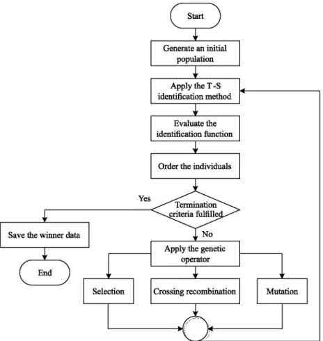
The proposed GA follows the next steps, shown in

Fig. 2:

1. An initial population, composed by a set of individuals, is

defined. Each individual of the population is formed by a

fuzzy system, made by n

fuzzy rules. In each fuzzy rule, a

set of antecedents is determined, {z{\ e $ and {pj e W,

which defines a MDMF. The initial antecedents of the fuzzy

system are specified for each individual with different

val-ues. Thus, firstly, the number of fuzzy rules n

, the number of

( Start J

Generate an initial population

Apply the T-S identification method

Evaluate the identification function

Order the individuals

Yes

Save the winner data

f End J

Apply the genetic operator

Selection Crossing recombination Mutation

Fig. 2. GA for MDMFs adjustment. For each individual of the population in the current

genera-tion, a T-S identification based on MDMFs is performed, ob-taining the T-S consequents of each fuzzy rule, as is shown in Section .

The identification results of each individual are verified with respect to a function E, defined as the weighted mean for each output of the Root Mean Squared Error (RMSE) of the identification error.

i = l

RMSE(yt(.k)-Mk))

s • RMSE (yj(k)) (11)

The objective of the GA is minimizing the function E, thus minimizing the identification error, through the optimal adjustment of the MDMFs parameters (zt and pt).

4. The population individuals are ordered in the current gen-eration according to their value obtained in the evaluation function E, from low to high. The individual which has the lower value in E, will become the winner of the population in the current generation.

5. The termination criterion is checked. If the specified max-imum number of generations is reached or the value in E obtained by the winner is less than a defined value, then the algorithm ends and the T-S antecedents and consequents of the winner are saved. If the termination criterion is not fulfilled, the algorithm continues.

6. The following genetic operators (selection, cross recombina-tion and mutarecombina-tion) are applied on the ordered popularecombina-tion of individuals in the current generation to obtain a new pop-ulation of individuals for the next generation. The genetic operators are only applied to the T-S antecedents.

• Selection: the winner is chosen for the next generation. This operator ensures that an optimal individual could be preserved through generations.

• Cross recombination: some descendants for the next generation are generated by the combination of the best individuals. These operators allow to look for an optimal individual near the best individuals, therefore it allows a small range search but very deep one. • Mutation: some (or all) characteristics of some

indi-viduals are randomly modified for the next generation. These operators are necessary to avoid local minima, since its random search can be made in the full range. Then, the algorithm continues in step 2, updating the popula-tion of individuals for the next generapopula-tion.

The objective function of the GA is designed to minimize the T-S identification error. In other words, the proposed GA is applied to find the best parameters for MDMFs which minimize the T-S identification error.

The proposed method has no restrictions on the GA param-eters, operators and their implementation. Thus, without loss of generality, more details about how the proposed method can be applied and the genetic operators can be defined, are presented in Section 5.

A faster convergence of the algorithm has been obtained by taking the centre point (zf) of the central MDMF of each individual

as the gravity centre of the system data, since it is the most repre-sentative point. In this way, this centre point of the central MDMF is kept constant throughout the GA generations, facilitating the convergence of the rest of the MDMFs to their optimal locations.

u2

^1 hi

Qj

I hi*

Fig. 3. Coupled tanks system.

of fuzzy rules, which have a set of T-S a n t e c e d e n t s (defining t h e MDMFs) and T-S c o n s e q u e n t s (modelling t h e system d y n a m i c behaviour). Thus, t h e proposed m e t h o d works w i t h a huge set of p a r a m e t e r s , w h i c h are t r e a t e d as follows: t h e GA adjusts t h e T-S a n t e c e d e n t s of t h e fuzzy rules, while t h e T-S identification m e t h o d obtains t h e T-S c o n s e q u e n t s for each fuzzy rule.

Note that, t h e proposed approach develops an identification of nonlinear multivariable systems in an offline stage, t h u s t h e c o m p u t i n g time is not a d e t e r m i n i n g factor in t h e MDMFs pa-r a m e t e pa-r s a d j u s t m e n t algopa-rithm. On t h e othepa-r hand, pa-reducing t h e computational cost in t h e MDMF function (7) is necessary since this function should also be i m p l e m e n t e d in t h e fuzzy controller, which is usually an online stage.

5. Illustrative e x a m p l e

The p r e s e n t e d m e t h o d is proposed to be applied to any n o n -linear system identification based on Takagi-Sugeno fuzzy model. The m e t h o d could be applied to a n y nonlinear system w i t h any n u m b e r of fuzzy variables.

In this section, it is s h o w n t h r o u g h an illustrative example, a coupled tanks system, t h e advantages of t h e proposed T-S model based on MDMFs adjusted by a GA, in comparison w i t h T-S m e t h o d based on fuzzy inference of lDMFs. A coupled tanks system has b e e n chosen since this example fulfils all t h e advantages and s h o w s a clear graphical r e p r e s e n t a t i o n of the p r o b l e m and its solution.

5.2. Coupled tanks system

A coupled tanks system [38], s h o w n in Fig. 3 , consists of t w o vertical tanks interconnected by a flow pipe, which causes t h e levels of t h e t w o tanks to interact. Each t a n k has an i n d e p e n d e n t fluid valve for liquid inlet ( u1 ; u2) and a liquid outlet flow (Ch, Q2

)-Also, t h e r e is a flow rate Ch in t h e pipe connecting t h e t w o tanks. Considering mass balance, t h e dynamic equation of each tank is developed as follows:

Ui-(h-Q3=A1

-0.2 + 03= A. dt dh ' dt

w h e r e h\ and h2 are t h e heights of liquid in each tank. A\ and A2

are t h e cross-sectional areas of each tank.

Applying Bernoulli's equation for a non-viscous incompressible fluid in steady flow:

a2^2gh2

Qi

Q2

Q3 = sign (hj - h2) a3^2g\h1 - h2\

w h e r e a\, a2 and a3 are proportionality constants w h i c h d e p e n d

on t h e coefficients of discharge and t h e cross-sectional area. The connection flow rate Ch is a s s u m e d positive if hi is higher t h a n h2.

800

600

400

200

0

I

800

600

400

200

0 0.1 0.2 0.3 0.4 0.5 0.6 0.7 0.8 0.9 Ql

0

"_^r-rrT

0 0.1 0.2 0.3 0.4 0.5 0.6 0.7 0.8 0.9 Q2

Fig. 4. System data histograms.

Mlij 0.5

0 0.1 0.2 0.3 0.4 0.5 0.6 0.7 0.8 0.9 Ql

fei2 0.5

0 0.1 0.2 0.3 0.4 0.5 0.6 0.7 0.8 0.9 Q2

Fig. 5. lDMFs applied for T-S model.

Supposing t h e following process values:

A1 = A1 = 1 m2

a-[ = a2 = c<3 = 0.1

g = 9.8 m / s2

5.2. T-S identification of a coupled tanks system

The coupled tanks system can be modelled taking as state variables the output flow rates 0\ and Q2, with two inputs u\ and

u2. The sampling time for the discrete model is supposed to be

7" = I s .

Fig. 4 shows the system data histograms. Since the fuzzy vari-ables are selected as the state varivari-ables themselves (Ch and Q2), based on the histograms of the system data, it seems reasonable to define the lDMFs as three triangular functions overlapped by pairs

(Fig. 5).

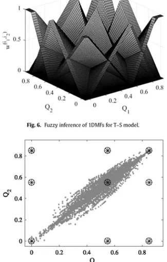
Thus, the fuzzy rules (Fig. 6) for the T-S model [2,7] are obtained by the fuzzy inference of the lDMFs:

S(il-i2): If Qi(fe) isMJ1 and (>,(/<) isMJ then:

model becomes:

S

-

: If (h{k) isMJ

and Q

(k) isMJ then:

Fig. G. Fuzzy inference of lDMFs for T-S model.

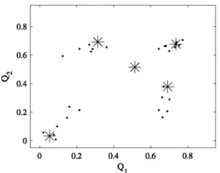
Fig. 7. Fuzzy inference central points projected over the system data space.

Fig. 7

represents the central points of the functions obtained by

fuzzy inference, projected over the two-dimensional space of the

system data.

The linearized model parameters Po are calculated using the

classical least squares method over the system data, with an

es-timation error of 0.0101.

Qi(fc+1)

Q^fc+l)

aio

O20

fan bi2

^ 2 1 ^22

O i l Ol2 021 #22

u

(k)

Qi('<)

Q2('<)

OlO Oil Ol2 fall bn

°20 °21 °22 ^21 ^22

0.0014 0.6066 0.2064 0.1262 0.0585

0.0005 0.1918 0.6238 0.0584 0.1246

With the linearized system parameters P

, the 1 DMFs shown in

Fig. 5

and the weighting factor y = 10~

, obtained by trial and

error, an estimation error of 0.0043 is obtained using the above

T-S identification method developed by the authors in

[7,8].

The T-S

=

+

" a(iuh) ' Huh)

. U2 0

" 1 1 b( i l , b ) . " 2 1

+

fa

fa

. 02 1. 1 1. 1

2) „(>1.>2 U1 2 2) Jh,h

u2 2

" Ul(><) "

_ u

(k) _

)

)

" Qi(k) "

_ (h(k) _

Qi(fc+l)

Q 2 ( k + i )

In

Fig. 7,

it can be seen how the fuzzy inference of lDMFs

produces fuzzy rules far from the system data, such as those at the

top left and bottom right, which have no relevance to the

iden-tification algorithm. These fuzzy rules introduce an unnecessary

computational cost for the control stage, since the fuzzy controller

must consider more fuzzy rules than those which are indeed used.

Note that these fuzzy rules away from the system data

(Fig. 7)

have been produced by the fuzzy inference process and they have

not been generated by a design error, since the lDMFs

(Fig. 5)

have been confirmed with the system data histograms

(Fig. 4).

The

generated fuzzy rules by the fuzzy inference process are usually

not optimal and sometimes do not even correspond to the system

data.

5.3. Modelling and identification of a coupled tanks system applying

the proposed method

As it has been described above, the coupled tanks system is

modelled by taking the output flow rates Ch and Q2 as state

vari-ables, with two inputs U\ and u

. Thus, the proposed T-S model

based on MDMFs becomes:

S

:Ifz(k)isM

then:

=

+

°io

. ° 2 0 .

fa'

" 1 1

fa'

. " 2 1

+

fa'

" 1 2

fa'

" 2 2

a

a

' a'

11 u1 2

' a'

21 u2 2 _ " Ul(><) "

_ u

(k) _

' Qi('<) "

_ (h(k) _

Qi(fc+l)

Q^fc+l)

where the fuzzy variables are the state variables themselves:

z=[Qi 0 2 ] '

Five fuzzy rules are used to define the T-S fuzzy system. The

number of fuzzy rules have been defined through a trial and error

adjustment over the proposed example. Many trials have been

made. It has been found that five fuzzy rules offer a good

compro-mise between computational cost and identification error.

In the GA, the population is formed by fifteen individuals. The

GA ends when one hundred generations are reached. In order

to obtain the next generation of individuals, the applied genetic

operators, in the ordered population of individuals, are:

• For individual 1: Selection. The winner is updated for the next

generation without changes.

• For individuals 2,3,4,5: Cross recombination. These

individ-uals are combined with the winner for the next generation.

- Individuals 2 and 3: The parameters are obtained from

the winner, but the parameters of one of the rules are

obtained taking the mean of these parameters from the

winner and individuals 2 and 3 respectively.

- Individuals 4 and 5: The parameters are obtained from

individuals 2 and 3 respectively, but the parameters of

one of the rules are obtained taking the mean of these

parameters from the winner and individuals 2 and 3

respectively.

o

0.8

0.6

0.4

0.2

0

•

m

- • * '

. # •

•

*

.

-/fc

*

• •

-0 -0.2 -0.4 -0.6 -0.8

Fig. 8. MDMFs centres of the winner at each iteration. Fig. 9. System data and obtained MDMFs centres.

- Individual 6: The parameters are obtained from the

winner, but random increments over the parameters of

one of the rules are added.

- Individual 7: The parameters are obtained from the

winner, but a random increment over the position

pa-rameter Zj of one of the rules is added.

- Individual 8: The parameters are obtained from the

win-ner, but a random increment over the distance

weight-ing parameter pj of one of the rules is added.

- Individual 9: The parameters are obtained from

individ-ual 2, but random increments over the parameters of

one of the rules are added.

- Individual 10: The parameters are obtained from

in-dividual 2, but a random increment over the position

parameter Zj of one of the rules is added.

- Individual 11: The parameters are obtained from

in-dividual 2, but a random increment over the distance

weighting parameter p

of one of the rules is added.

• For individuals 12 and 13: Large mutation. Large random

changes are applied over the winner. The parameters are

obtained from the winner, but the parameters of one of the

rules are randomly chosen.

• For individuals 14 and 15: Complete mutation. New random

individuals are generated for the next generation.

In the complete algorithm, there are fifteen individuals in the

GA population. Each one with five fuzzy rules. Each fuzzy rule

has as T-S antecedents the MDMF parameters, the centre point

Zj G Ot

and the distance weighting p

e Ot

. Moreover, each fuzzy

rule has as T-S consequents, ten parameters of the T-S fuzzy state

model. Thus, the algorithm works with 1050 parameters (15 • 5 •

(2 • 2 + 10)). Thus, the proposed algorithm works as follows:

• The GA manages the T-S antecedents of each individual for

all fuzzy rules (20 parameters (5-2-2) per individual).

• With the defined fuzzy rules, the T-S consequents of each

individual are obtained by T-S identification method [2] (50

parameters (5 • 10) per individual).

Applying the GA for MDMFs design with the above described

characteristics, the following results are obtained:

Fig. 8

shows the MDMFs centre points of the winner at each

iteration. Note that the centre point (z

) of the central MDMF

remains static throughout the GA generations, because it is defined

as the centre of gravity of the system data.

Fig. 9

shows the centre points of the MDMFs obtained at the end

of the GA algorithm over the system data.

-,

0.5

-Fig. 10. MDMFs obtained with the proposed algorithm.

In

Fig. 10,

the final MDMFs obtained for the fuzzy system with

the proposed algorithm are shown.

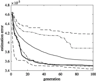
Since the GA has an important random component, one

hun-dred tests have been performed and the results of the estimation

error of T-S identification using MDMFs, throughout the GA

gen-erations, are shown in

Fig. 11.

The mean of the T-S identification

error during the GA generations is represented in continuous line.

Maximums and minimums are drawn in dashed line. Percentiles

10 and 90 are shown in dash-dot line. The T-S identification error

through the GA generations obtained in this work shown test is

represented in thick continuous line.

It can be seen in

Fig. 9,

that the fuzzy rules are not restricted to

lDMFs elements combination, such as using the fuzzy inference

method

(Fig. 7).

The use of MDMFs allows that the fuzzy rules

can be placed at any point of the multi-dimensional space. Thus, a

better adjustment over the system data can be obtained, improving

the identification results through a smaller number of fuzzy rules.

An estimated error of 0.0035 is obtained. In addition, the results

obtained with the T-S identification

[7,8]

have been performed

with 9 fuzzy rules, whereas in the proposed identification method

only 5 multidimensional fuzzy rules have been used. Thus, not only

better results are obtained in the identification, but it has been

reduced the number of fuzzy rules.

It can be seen in

Fig. 11

how the identification error decreases

throughout the GA generations. All the tests give similar results,

obtaining better results than the T-S identification method

[7,8]

4.8 4.6 4.4

" 4.2 c o

1 *

•a

u3 . 8

3.6 3.4

xlO""

V-s

i\Vx —

-i V \

i \ \ .

•

-^

20 40 60

generation

80 100

Fig. 11. Estimation error of T-S identification using MDMFs throughout the GA

generations, (a) Continuous line: mean of 100 tests, (b) Dashed line: maximum and minimum of 100 tests, (c) dash-dot line: percentiles 10 and 90 of 100 hundred tests, (d) Thick continuous line: test shown in the article.

Table 1

Probability of occurrence of the genetics operators.

Individual Occurrence (%)

1 2 3 4 5 6 7 8 9 10 11 12 13 14 15

61.95 6.09 5.94 1.72 0.97 2.75 2.45 7.70 1.73 1.61 5.24 0.88 0.87 0.03 0.07

the occurrence probability of the genetic operators applied over the individuals previously defined is shown in Table 1.

6. Conclusions

In this paper, a new method for the T-S model identification of nonlinear multivariable systems using MDMFs is developed. The fuzzy inference method of lDMFs can produce fuzzy rules that do not correspond to system data. This in turn produces a loss of optimality and an unnecessary computational cost. MDMFs are proposed for solving this problem.

The proposed algorithm for the T-S identification using MDMFs consists in the adjustment of T-S antecedents (the MDMFs param-eters) using a GA and the calculation of the T-S consequents using the T-S identification method.

An illustrative example shows that the proposed method pro-vides a fewer identification error with a smaller number of fuzzy rules than the lDMFs fuzzy inference method.

Acknowledgements