Geometric characteristics of conies in Bézier form
A. Cantón
3, L Fernández-Jambrina
3, E. Rosado María
ba Departamento de Ciencias Aplicadas a la Ingeniería Naval, E.T.S.I. Navales, Arco de la Victoria s/n, E-28040-Madrid, Spain
b Departamento de Matemática Aplicada a la Edificación, al Medio Ambiente y al Urbanismo, E.T.S. Arquitectura, Juan de Herrera 4, E-28040-Madrid, Spain
A B S T R A C T
Keywords:
Conic sections Bézier curves Eccentricity Asymptotes Axes Foci
In this paper, we address the calculation of geometric characteristics of conic sections (axes, asymptotes, centres, eccentricity, foci) given in Bézier form in terms of their control polygons and weights, making use of real and complex projective and affine geometry and avoiding the use of coordinates.
1. Introduction
Arcs of conic sections are easily represented as quadratic rational curves and this is the way they have been implemented in Computer Aided Geometric Design in exact form. Since they appear in almost every branch of industry, conic sections by themselves justify the inclusion of weights and denominators to extend polynomial curves in Bézier representation to rational ones.
Deriving closed formulae for geometric characteristics of conies given in Bézier form, that is, in terms of their control polygon and weights, was first accomplished in some cases in [1] by the use of metric or Euclidean geometry. They may be found also in [2].
In [3], a different approach is followed, grounded in the calculation of the foci as intersections of the tangents to the conic from the circular or absolute points. The main advantage of this approach is that the results are common for ellipses, hyperbolas and parabolas.
In [4], closed formulae are obtained for computing geometric characteristics of conies from the invariants of rational quadratic parameterisations under rational linear reparameterisations in-stead.
On the other hand, in [5], recipes are produced for constructing Bézier representations of conies when some of their geometric characteristics are known. In [6], complex arithmetic is used to calculate some geometric characteristics of conic sections.
Most recently, in [7], the eccentricity of conies in Bézier form is formulated and this result is used for deriving the range and extreme values of this parameter.
As a different approach, we resort to projective and affine geometry to calculate geometric characteristics of conic sections in
Bézier form. Some concepts such as centre, foci and asymptotes can be defined at this level without introducing additional structure (scalar product, angles and lengths), though other geometric characteristics, such as axes, semi-axis lengths and eccentricity require calculation of angles and lengths and require therefore resorting to Euclidean geometry. The novel point in our approach is the possibility of writing the implicit equation of the conic in a coordinate-free expression that just uses the vertices and sides of the control polygon and the weights. This enables us to write geometric characteristics in closed form in a coordinate-free fashion.
In Section 2, we provide a quick review of some concepts of projective and affine geometry, which we use in Section 3 to write down the implicit equations of a conic arc in Bézier form. This form of writing the equations is determinant for deriving expressions for geometric characteristics of conies in Section 4.
2. Preliminaries and notation
We start by reviewing some concepts of projective geometry, that may be checked in more detail elsewhere (cf. for instance [8,9]). Previous applications of projective geometry and point-line dual representations maybe found in [10,11].
In affine geometry, the Euclidean concepts of angle and length are lost and vector lengths can be compared only along parallel directions through the ratio of two vectors or three collinear points. Parallelism remains as an affine notion whereas perpendicularity does not. In projective geometry, the cross ratio of four collinear points is preserved instead of the ratio. The notion of parallelism is lost since every pair of lines on the projective plane meet at one point. The projective plane may be modelled by adding a line at
infinity to the affine plane, formed by the points where parallel
a+p+y=0
Fig. 1. The affine plane as subset of the projective plane.
The projective plane is the set of vector lines of R3. Each point X of the projective plane is then characterised by a vector v or its
multiples Xv, for any X=£ 0.
A frame of the projective plane is a set {P, Q, R] of non-aligned
points. That is, if we choose vectors {v-i, v2, v3] along these lines as
their respective representatives, they form a basis of R3. Hence, we
may write any point X of the projective plane as a combination
X = aP + PQ_ + yR, (1)
which just states that there is a representative v ofX which satisfies
v = ai\ + Pv2 + yv3.
Expression (1) is unambiguous provided that the choice of vectors {v\,v2,v3} is fixed. However, the set of coordinates
(a, p, y) ofX in this frame is equivalent to (Xa, Xp,Xy) f o r i ^ 0,
since this linear combination produces a vector Xv which is also a representative ofX. Hence, the coordinates of a point X in a frame are defined up to a non-zero multiplicative factor.
Once a frame has been chosen, we may distinguish two types of points of the projective plane:
- Points with coordinates (a, p, y) such that a + p + y ^ 0. We may choose another set of coordinates (a, p, y) =
(Xa, X/3, Xy), with X = l / ( a + p + y) so that these points are viewed as bary centric combinations áP + PQ + yR,á + p + y =
1, of {P, Q, R}; see Fig. 1. The frame in the projective plane provides a frame in the affine plane.
Hence the plane in R3 of equation a + p + y = l i s a n affine plane and its points are written as barycentric combinations of
the frame {P, Q, R}.
- Points with coordinates (a, p, y) such that a + p + y = 0. It is clear that these are not points of the affine plane. These points of the projective plane form the line at infinity of equation
a + P + y = 0 . They are the directions of vectors of the affine
plane introduced in the previous paragraph; see Fig. 1.
We use capital letters for points in the projective plane, which may be either points in the affine plane or points at infinity. ByXY we denote the vector linking the points X and Y in the affine plane. A line / in the projective plane is a vector plane of R3. We may
assign to it a linear map / so that /(X) = 0 is fulfilled by points X of the projective plane on the line /. For simplicity in the notation, we denote then by / both the line and a linear map that vanishes at points of the line /.that is, /(X) = OforX e /.Aline in the projective plane is formed by its points in the affine plane and a point at the line at infinity, which is the direction of the line. We use lower case letters for lines.
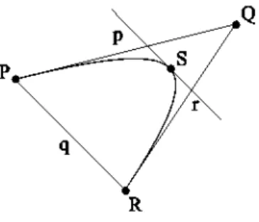
Now we consider conic arcs in Bézier form,
Fig. 2. Conic arc in Bézier form.
defined by their control polygon, {c0, C\, c2) (in what follows, we
denote P = c0, Q = Ci,R = c2), and their normalised weights,
{1, w, 1}. The arc starts at P = c(0) and ends at R = c(l). Our frame is then the control polygon of the conic arc.
We denote by p the line through P and Q, r is the line through
R and Q and q is the line through P and R. This choice reflects that
p, q, r are respectively the polar lines of P, Q, R, as will be shown below.
Since c'(0) = 2wPQ andc'(l) = 2wQR, the conic arc is tangent to p and r at P and R, respectively (see Fig. 2).
The linear maps p, q, r are fixed up to a multiplicative factor, which we may fix requiring that
p(R) = l, q(Q) = l, r(P) = l. (2)
This means that {r, q, p] is the dual basis for {P, Q, R) since
p(P) = 0 = p(Q), q(P) = 0 = q(R), r(Q) = 0 = r(R).
To avoid lengthy expressions, we shall denote the directions of the lines p, q, r as
••OP, RP, QR. (3)
A quick way to obtain the direction of a straight line I = jtp +
pq + or, with real coefficients it, p, a, is looking for a point at
infinity aP + /3Q + yR, a + /3 + y = 0 along the line,
0 = (np + pq + or)(uP + PQ + yR) =icy + pf3 + era.
A simple way of writing the solution to these equations is
a = X(p — TC), p = X(TC — a), y = X(a — p),
where X is a nonvanishing factor that we may take equal to one if we are just interested in the direction of the line:
Lemma 1. The direction of a straight line 1 = jtp + pq + ar is given by
(p - Tt)P + (?r - er)Q + (a - p)R,
or in terms of p and f,
(p - Tt)p + (a - p)r.
Conversely, the equation of a straight line through two points is readily written:
Lemma 2. The straight line I through two points, a^P + fiiQ. + y\R, a2P + p2Q + y2R, is given by
I = jtp + pq + ar,
c(t) c0(l - r)2 + 2wc1r(l - t) + c2t2
(1 - r )2 + 2wr(l -t) +t2
t 6 [0, 1],
«i u2 Y\ Y2
«i u2
Fig. 3. Examples of polar lines of points.
just finding solutions of the system of equations, i = 1,2,
0 = (?rp + pq + or) (a¡P + # Q + y{R) = u{a + frp + y¡jr.
The line at infinity is z = p + q + r, since its points are combinations aP + /3Q + yR with a + /3 + y = 0.
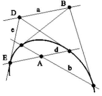
For a conic section, the polar line (cf. for instance [9] or [12]) of a point A is defined as:
- If A lies on the conic, the polar line of A is the tangent line at A. For instance, p is the polar line of P and r is the polar line of R. - If A lies out of the conic, we trace both tangents to the conic
through A. They meet the conic at two points. The line linking both tangency points is the polar line of A. For instance, q is the polar line of Q. If we cannot draw the tangents to the conic from a point A, we may obtain its polar line a by linking two points B and D with polar lines b, d meeting at A; see Fig. 3.
In what follows, the polar line of a point and the point will be denoted by the same letter in lower and upper case respectively, as we have already done in the previous paragraphs.
We may obtain the polar line a of point A analytically: if C is the symmetric bilinear form associated to the conic, so that C(X, X) = 0 for points X on the conic, the pointsX of a satisfy 0 = C(A,X).
3. Implicit equations of conic sections
For determining a conic section we require five points. Providing the tangents p at P and r at R amounts to four points, since P and R are then double points. There are two degenerate conies that satisfy these conditions: the intersecting pair of lines
C\ = p U r of quadratic form p • r (pr + rp as symmetric bilinear
form), which fulfils the tangency conditions at P and R, and the double line C2 = q U q of quadratic form q2, for which P and R
are double points.
Hence, all conies satisfying these conditions are members of a pencil of conies
, / p r + rp , \
pr + Xq , ( h Xq as a symmetric form I (4)
in terms of both degenerate conic sections.
It is obvious that P and R belong to the conies in the pencil, that is
p(P)r(P) + kq(P)2 = 0 = p(R)r(R) + kq(R)2.
Using the symmetric form of the pencil of conies (4), we show that a point X is on the polar line of P if and only if
r(P)p(X)+p(P)r(X) p(X)
0 = + kq(P)q(X) = —^-,
and hence p is the polar line of P. Similarly, we get r as the polar line of R and q as the polar line of Q,
r(Q)p + p(Q)r , . . . . + Xq(Q)q = Xq.
A fifth condition fixes the pencil parameter k and is obviously related to the weight w, which has not appeared so far. We may check it with the help of the shoulder point S [13],
S :=c ( l / 2 ) = P / 2 + W Q +*/ 2,
1 + w which satisfies the conic equation,
\/4 + kw2
0 = p(S)q(S) + kq(Sy X: 1
Aw2'
(1 +
w)2The w = oo case corresponds to the degenerate conic p U r, whereas the w = 0 case is the double line (¡Uq.
The polar line s of the shoulder point,
r(S)p + p(S)r
+ ^q(S)q
4(1 - — - (p + r )
is parallel to the line q,
s(9) = 7 7 7 ^ ^ (P(R) - r(P)) 0, 4(1 + w)
since it contains the direction q of q (see Fig. 2).
Analogously, we may think of a dual representation, exchanging the roles ofpoints and lines: a point /of the dual projective plane is a line and a line P of the dual projective plane is the pencil of lines through the point P. A line belongs to a conic C if it is a tangent to the conic.
We look for the tangential equation of our conic arc. That is, the implicit equation for the tangent lines to the conic.
Since p and r are respectively the tangents to the conic at P and R, there are already defined four conditions for the pencil of tangential conies.
We proceed again searching for two degenerate conies satisfy-ing these conditions:
The degenerate conic C\ = P U R of quadratic form PR (or
(PR + RP)/2 as a symmetric form) contains both p and r,
p(P)p(R) = 0 = r(P)r(R),
and p is the polar line of P,
p(P)R + p(R)p = p,
and analogously r is the polar line of R.
The other degenerate conic is C2 = Q U Q of quadratic form Q2,
since it contains both p and r,
P(Q)P(Q) = 0 = r(Q)r(Q), twice.
The pencil of conies tangent to p at P and to r at R is formed, then by linear combinations of both degenerate conies,
, {PR + RP
PR + /xQ2, + /¿QQ as a symmetric form J .
Obviously, the line p,
p(R)P+p(P)R P
+ MP(Q)Q = - ,
is the polar line of P and r is the polar line of R and q
g(R)P+q(P)R ,
+ M ( Q ) Q = nQ. is the polar line of Q.
Again, we can fix again the free parameter ¡i making use of the shoulder point S.
We already know that the tangent line s at the shoulder point has linear map s = p + r — q/w. Hence, from
0 = s{R)s{P) + /j,s(Q.y
1 +
we learn that ¡i = —w2.
Proposition 1. The implicit equation of a conic arc defined by its control polygon, {P, Q, R], and its normalised weights, {1, w, 1} is given by
p(X)r(X) g(X)2
Aw2
0.
Analogously, the tangential equation of the conic is
x{P)x{R) -w2x(Q_)2 = 0,
(5)
(6)
where p, q and r are respectively the linear maps corresponding to the polar lines of P, Q, R, as described in (2).
These expressions allow us to write in a straightforward and elegant manner the implicit equations of conies given in terms of their control polygons and weights, without making use of the coefficients of the conic equation,
a00 + amx + a02y + anx2 + anxy + a22y2 0,
The implicit equation of the conic in barycentric coordinates referred to the frame {P, Q, R] is the direct result of applying the implicit equation to a point X = aP + /3Q + yR,
0 = p{X)r{X) q{X)2 •• ay
Aw2 Aw2'
or for a straight line as a combination of p, q and r, x = 7tp +
pq + or, to be a tangent line to the conic,
0 = x{P)x{R) - w2x(Q_)2 : no — w2p2.
Corollary 1. The implicit equation of a conic arc defined by its control polygon, {P, Q, R], and its normalised weights, {1, w, 1} in barycentric coordinates referred to the vertices of the control polygon, aP + /3Q + yR,is given by
ay Aw2
0. (7)
Analogously, the equation for tangent lines to the conic in barycentric coordinates, referred to the sides of the control polygon, 7tp + pq + or, is
2 2
W p
o,
(8)where p, q and r are respectively the linear maps corresponding to the polar lines of P, Q, R, as described in (2).
4. Geometric characteristics of conies
4.1. Centres and diameters
A first instance of geometric characteristic of a conic which we characterise without making use of Euclidean geometry is the centre.
The centre C is, to this end, defined as the point of intersection of the diameters of the conic. Note that the diameters of the conic are the polar lines of the points on the line at infinity, since the tangents to the conic at the intersections with a diameter are parallel. Hence, the polar line of the centre is the line at infinity, z = p + q + r (see Fig. 4).
Hence using the tangential equation (6) of the conic, we get the centre as the point which has the line at infinity as polar line,
z(R)P+z(P)R , P + R
C w¿z(Q.)Q.
2 2 or writing it as a barycentric combination,
P +R-2w
2(l
• u r Q ,
C
Fig. 4. The centre of the conic as the intersection of diameters.
Fig. 5. The centre of a parabola lies at infinity.
for w ^ 1. The case w = 1 corresponds to the parabola. Another simple reasoning for calculating the centre of a conic is found in [ 1 ].
Diameters are straight lines passing through the centre. Hence a line 7tp + pq + or is a diameter if
0 = (jrp + pq + O T ) ( C )
7t + o — 2w
2p
2-2w
2The case of the parabola, w = 1, can also be included here from this perspective, though within Euclidean geometry it is a noncentral conic section. In this case, the centre
C P + R p + r
is a direction, not a point, since it is written as a barycentric combination in which the sum of the coefficients is zero. Hence, the centre of the parabola is its only point on the line at infinity, which is the direction of the axis of the parabola. The parabola is tangent to the line at infinity at its centre. Since all diameters meet at the centre of the conic, the diameters of the parabola are straight lines parallel to the axis (see Fig. 5).
Proposition 2. The centre of a nondegenerate conic arc defined by its control polygon, {P, Q, R], and its normalised weights, {1, w, 1} is given by
C P + R -2w2d
2-2w2 :
(p + r if 1 (9)
and the diameters are straight lines of equation Jtp(X) + pq(X) + or(X) = 0 satisfying
jt + o — 2w2 p = 0, (10)
2w2
where p, q and r are respectively the linear maps corresponding to the polar lines of P, Q, R, as described in (2).
4.2. Asymptotes
have a simple derivation within projective and affine geometry. A different approach to calculate them is used in [4]. More on asymptotes of rational Bézier curves maybe found in [10].
We get the directions of the asymptotes as the intersections of the conic with the line at infinity, searching for solutions
v = aP + PQ + yR, a + p + y = 0,
of Eq. (7). Taking ¡3 = —2w to avoid denominators,
v± = (w ± jw2 - i\ P - 2wQ + (w =F \IVJ2 - \ \ R
= (w ± Vio2 — l ) p + ( u ; = F V»)2 — 1) r,
Of course, for the parabola, w = 1, we get the centre twice,
v = p + r.
The asymptotes are easily computed now as the tangents or polar lines to these points at infinity,
0 = r(v±)p + p(v±)r q(y±)q
2w2
= (w ± V»)2 — 1) p + (w =p V»)2 — 1) r H .
For the parabola we get p + q + r = 0 twice, the line at infinity, as expected.
Proposition 3. The asymptotes of a nondegenerate conic arc defined by its control polygon, {P, Q, R},anditsnormalisedweights, {1, w, 1} have implicit equations
(w ± jw2 - \\ p(X) + (w T Vw2 - l ) r(X) + — = 0, (11) where p, q and r are respectively the linear maps corresponding to the polar lines of P, Q, R, as described in (2).
The directions of the asymptotes are
v± = (w ± -Jw2 — 1) p + (w =p -Jw2 — 1) r, (12)
where p = QP and f = QR.
4.3. Axes
For obtaining the axes, we finally need Euclidean geometry, but we may make use of our previous results. We denote by {v, w) the scalar product of two vectors v, w.
An axis is a diameter which is orthogonal to the tangent lines at the intersection points with the conic.
The axis of a conic is one of the diameters d = 7tp + pq + or satisfying Eq. (10),
jr + a — 2w2p = 0.
Following Lemma 1, its direction is
v = (p - Jt)p + (a - p)r,
On the other hand, a diameter d is the polar line of a point D at infinity,
d{R)P + d{P)R
D = = w d(Q_)Q_
jtP +aR w2pQ,
2 ^ ' ^ 2
which is the direction of the tangents to the conic at the points where it intersects the diameter (see Fig. 4).
If these points are vertices of the conic section, the direction v of the diameter is orthogonal to the direction D of the tangents at the vertices,
0 = (jrp + or, {p - Tt)p + {a - p)r)
= 7t(p — jr)||p||2 + p{a — jr)(p, r) + a{a — p)\\r\\
We may solve (10) and remove the ambiguity in the coefficients
n,p,a by fixing
jr — a = 2, jr = w2p + 1, a = w2p — 1,
so that Eq. (13) takes the form
Sl|2 w2(w2 - \)p2 +
2w2(||r||2 + ||p||2)
-p + 1 = 0 , (14)
which provides the two axes:
Proposition 4. The equations of the axes of a conic defined by its control polygon, {P, Q, R},anditsnormalisedweights, {1, w, 1}, w ^
1, are np{X) + pq(X) + ar{X) = 0, with coefficients given by
w p + 1, a = w p 1
and p isa solution of (14), except for the case of an isosceles polygon,
||p|| = \\r\\, for which the coefficients satisfy either it = —a = 1,
p = 0orjt=a = w2, p = 1.
The directions of the axes are
v\ = (p — Jt)p + (a — p)r, v2 = up + or,
as linear combinations of the vectors introduced in (3).
The case of the parabola is simpler, since we already know that the axis has the direction given by the centre, a point at the line at infinity p + r, and is one of the diameters d = 7tp + pq + or satisfying (10),
jr + o — 2p = 0.
The diameters intersect the conic at its centre and at another point (see Fig. 5) and the direction of the tangent at it is 7tp + of. If this point is the vertex of the parabola, V, the direction p + r of the axis is orthogonal to the direction of the tangent at the vertex,
0 = (jrp + of, p + r) = jr||p||2 + (jr + o)(p, f) + o\\f\\2,
and we may read the coefficients of the equation of the axis,
jr = 2(r,p + r) P -2{p,p + f)
which can be obtained as the case w = 1 of (14).
The vertex is obtained by intersecting the axis with the parabola:
Proposition 5. The equation of the axis of a parabola defined by its control polygon, {P, Q, R] is
2(r, p + f)p + (\\f\\2 — ||p||2) q — 2{p, p + f)r = 0,
where p, q and r are respectively the linear maps corresponding to the polar lines of P, Q, R, as described in (2) and p = QP, f = QR.
The vertex of the parabola is given by
f,p + f)2P + 2{p, p + f){f, p + r)Q_ + (p, p + f)2R
V
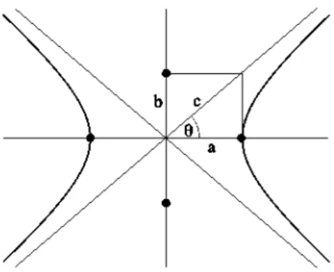
4.4. Eccentricity
\\p + r\\
Let a be the length of the semi-major axis (the one containing the foci), b the length of the semi-minor axis (the one containing the foci) and c the semi-focal distance. The eccentricity of a nondegenerate conic is defined as the quotient
(13)
0
4a
2-b
2a
1
Va
2 + b2< 1
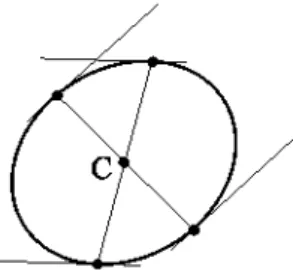
circumference
ellipse
parabola
Fig. 6. Asymptotes of a hyperbola and its eccentricity.
taking into account that for the ellipse a2 = b2 + c2 and for the
hyperbola c2 = a2 + b2.
It is possible to use our expressions for the asymptotes in order to calculate the eccentricity of a conic section, instead of using the lengths of the axes.
If we consider a hyperbola, the angle 9 (see Fig. 6) between any of the asymptotes and the major axis is related to its eccentricity,
1 cos 9 = -.
e
Since the axes produce lengthy expressions in Bézier form, it is more convenient for our purposes to use the angle 29 between the asymptotes,
n2 _b2 2
cos 29 = cos 9 — sin 9 cr 1,
taking into account that we already know the asymptotic directions v± obtained in (12),
{v+, t>_) = ||p||2 + ||r||2 + 2(2w2 - l)(p, r)
= UP — ?ll2 + 4w2{p, f),
where the sign has been chosen in order to produce the correct definition oí9 and not the complementary angle.
\v±\\ (2w2 - 1)
± 2w^w2
\\P\\2 +
\\P\\4 +
+ 2{p,f)
+ 4(p, r)2 + 2(8w4 - Sw2 + l)||p||2||r||2
+ 4(2w2 - l ) ( p , r )
( | | q | |2- 2 u ;2( | | p | |
+ 4w2(l - w2) ( | | p | |
llp||
2+
+ llrl
2))
Naming
wz wz
following the notation in [7], we get the formulae for the angle
{v+, V-) —b
~
JA'cos 29
and the eccentricity of the conic section,
1 + cos 26»
2^~A
(16)
A similar reasoning may be applied to ellipses, with complex asymptotes instead, leads to the same result:
Proposition 6. The eccentricity of a conic arc defined by its control polygon, {P, Q,R], and its normalised weights, {1, w, 1} is given by (16), where p = QP, q = RP, f = QR
If the conic section is a hyperbola, the angle between its asymptotes is given by (15).
Fig. 7. Foci and directrices of a conic.
4.5. Foci
A central conic has four foci (two real and two complex ones) which are constructed as the intersections of the isotropic lines, which are the tangents to the conic drawn from two complex points located at the line at infinity named absolute or circular
points I, J. The polar lines of the foci are called directrices.
The circular points [9,12] are the points at the line at infinity where all circumferences meet. They are also the only points of the projective plane which are invariant under translations and rotations. The invariance under translations requires that the circular points cannot be points of the affine plane, but vectors. And the invariance under rotations requires that they have zero length. A consequence is the remarkable property that they have the same coordinates in every cartesian frame. In this section, the bar denotes complex conjugation and i is the imaginary unit V—l".
As we see in Fig. 7 (note that the diagram is fictitious due to the impossibility of drawing it in the complex plane), the polar lines i, j of the circular points provide the four tangency points of the isotropic lines. We may draw six lines through couples of these points. Four of them are the directrices.
The vanishing modulus conditions allow us to write the circular points as complex barycentric combinations of {P, Q, R],
aP + bQ + cR, - Ilrll P'V/2 r
J
aP + bQ + cR,\\e-i,p/2, b =
where q> is the angle between p and r.
Though these expressions are valid for every system of coordinates, it is useful for practical purposes (for instance, the examples at the end of the paper) to write down the expressions of a set of coefficients a, b, c in cartesian coordinates.
Noticing that a, b and c are defined up to a factor, we can also write these coefficients as
a = (Rx-Qx)+i(Ry-(ly),
(15) b = (Px - Rx) + i(Py - Ry), c=(Qx-Px)+my-Py),
where (Px,Py), (&, Qy), (Rx, Ry) are the coordinates of P, Q, R in
any given frame.
The linear maps of the polar lines of the circular points are then
i = ap + cr j = ap + cr
2w2
2w2
in terms of the lines p, q, r.
Hence the tangency points aP + /3Q + yR of the isotropic lines of/ to the conic section satisfy both
ay + ca 0, ay 0,
2w2 Aw2
The simplest case is that of a parabola. The polar lines of the circular points are diameters of the conic section since the circular points lie at infinity and hence they meet at the centre of the conic. But the centre of a parabola is a point of the parabola. Hence, the four tangency points reduce to three: twice the centre and two other points. The parabola has then just one directrix (and one focus), defined by the two non-central tangency points.
The two solutions of Eq. (17) for w = 1 are the centre C =
P + R - 2Q and
a c T = -P - 2Q + -R.
c a
The directrix/, the line through T and f is, following Lemma 2, / = jtp + pq + or, with
a a c c c c a a
4isin<p,
4isin<p,
P ac
at
ac
ac
-2isin2<p,
or multiplying it by ||p|| ||r||/4isin<p, in order to get simpler real coefficients,
/ = \\r\\2p — (p, r)q + \\p\\2r.
The focus F of the parabola is the point which h a s / as polar line:
Proposition 7. The equation of the directrix of a parabola defined by its control polygon, {P, Q, R] is
||r||2p(X) - {p,f)q(X) + ||p||2r(X) = 0,
where p, q and r are respectively the linear maps corresponding to the polar lines of P, Q, R, as described in (2) and p ••
The focus of the parabola is
\\r\\2P + 2(p, r)Q + ||p||2K
QP, r = QR.
\\p + r\\2
The case of central conies is more involved. Taking /3 = 2w,
y = \/a for simplicity, Eqs. (17) reduces to
wca bu + wa = 0, (18)
for the intersections of the polar line of/ with the conic. The two points T± of intersection of the polar line of/ have
a±
y±
b±
1
a±
Vb
2 2b
— 4w2ac
wc
=F s/b2 - Aw
2wa
«
P
2ac
2w,
(19)
as barycentric coordinates.
Their complex conjugatesare the coordinates of the intersec-tions T± of the polar line of / with the conic. Note that this fact relies on keeping the same choice of the branch of the root in (19). Otherwise, the roles of T+ and T_ would reverse.
In [3], the foci are constructed using the intersections of the tangents to the conic section from thecircular points.
The pairs {T+, f+} , {T+, f_}, {r_, f+}, {r_, f_} define the four
directrices of the conic section. We are interested mainly in the two real directrices.
According to Lemma 2, it is clear that the two real directrices
f± are those spanned by { r+, T+} and {r_,T_}, since their
expressions f± = jr±p + p±q + a±r have coefficients
7t± = 2w(a± — a±), P± = y±«± -u±Y±
l«±l
2o± = 2w(y± - y±) = 2w a± — a±
l«±l
2Fig. 8. Geometric characteristics of a parabola.
which may be simplified and made real dividing them by 2(a± — ¿ ± ) / l « ± |2.
Hence, the linear maps of the real directrices of the conic section are
/± = w\a±\ p — ÍR(a±)q + wr, (20)
where Dt(ai±) = (a± + a ± ) / 2 is the real part of a±.
The real foci F± are the points which have the directrices f± as polar lines:
Proposition 8. The equations of the real directrices of a central conic defined by its control polygon, {P, Q, R] and its normalised weights,
{1, w, 1}, are
w|a±|2p(X) - ÍR(a±)q(X) + wr{X) = 0,
where the coefficients a± are defined in (19) and p, q and r are respectively the linear maps corresponding to the polar lines of P, Q, R, as described in (2).
The respective foci of the conic are
F± | a±|2P + 2u;0fi(a<±)Q+K
| a±|2 + 2u;0fi(a<±) + l
5. Examples
We end up with some examples of application of our results to the determination of geometric characteristics of conies. Though our formulae do not depend on the choice of coordinates (barycentric or cartesian) made and are valid for all of them, we express points in usual cartesian coordinates in the affine plane. That is, the coordinates of a point are of the form (1, x, y) referred to an orthogonal basis.
5.1. Example of a parabola
We consider a parabola defined by its control polygon
P = ( 1 , 0 , 0 ) , Q = ( 1 , 1 / 2 , 0 ) , R = ( 1 , 1 , 1 ) ,
QP = ( 0 , - 1 / 2 , 0), QR = (0, 1/2, 1),
P(x, y) = V, Q(x, y) = 2x - 2y, r(x, y) = 1 - 2x + y.
The geometric characteristics of this parabola are drawn in Fig. 8. The cartesian equation of the parabola is
0 = p{x,y)r{x,y) <i(x,y)2 0.
The centre (direction of the axis) of the parabola is
V
Fig. 9. Geometric characteristics of a hyperbola.
The vertex of the parabola is
(r, p + r)2P + 2(p,p + r>(?, p + r)Q + (p, p + r)2R
||p + r||4
= 0 , 0 , 0 ) .
The equation of the axis a is
2(r, p + ?>p + (||r||2 — ||p||2) q — 2(p, p + r)r = 2x = 0.
The focus of the parabola is
\r\\2P + 2(p, r)Q + 2K 1
, 1,0,
p + r||2 \ 4
And the equation of the directrix d is
ll?ll2P — (P, ?)<J + llp||2r = y H— = 0.
4
5.2. Example of a hyperbola
We compute the geometric characteristics of a hyperbola with control polygon
( 1 , 4 , 0 ) , Q = ( 1 , 4 , 1 ) , R: 1,5,
and normalised weight w = 3 ^ 2 / 4 . Hence
5s QP = ( 0 , 0 , - 1 ) , QR.
9"
0, 1,
RP 0, - 1 ,
p(x, y) = x - 4
5x
q{x,y) = 9+y 9x
r(x,y) 4 - y ,
which are drawn in Fig. 9.
The cartesian equation of the hyperbola is
0 = p{x,y)r{x,y) g(x,y)2 _ x2 2y2
Aw2 ~ 8 9
0.
This is the equation of a hyperbola centred at the origin with axes coincident with the cartesian axes and semiaxis lengths equal to 4 and 5. We get these results within our formulation:
The centre of the hyperbola is
C P +R-2w2Q ( 1 , 0 , 0 ) .
2 - 2 w2
The asymptotes have Eqs. (11),
V2
24 (3x ± Ay) = 0.
Fig. 10. Geometric characteristics of an ellipse.
The angle between the asymptotes has cosine 7/25 and the eccentricity is 5/4, respectively computed with (15) and (16).
The equations of the axes are np{x, y)+pq(x, y) +ar(x, y) = 0, with coefficients ?r = w2p + \a = w2p — 1, satisfying (14),
i 8
9p2 80p + 64 = 0 =^ p = 8,
-and hence the equations of the axes read
8y
2x = 0, — = 0,
9
as expected.
The foci of the hyperbola are
F± \a
±\2P + w(a± +óe±)Q_+R
\a±\2 + w(a± +a±) + 1
(1, ± 5 , 0 ) ,
where
3 ^ 2 ,V2
~~A
'IT'
3^2 3^2
—
+ Í^ '
are obtained through (19).
5.3. Example of an ellipse
Finally, we provide an example of an ellipse with vertices
P = ( 1 , 3 , 0 ) , Q = ( l , 3 , 5 V 3 ) , R
and normalised weight w = 1/2. Hence
QP = (0, 0 , 5 ^ 3 ) , Q R = ( 0 ,
-3 5^-3
5 ^ 3
RP
p(x, y)
9 5 ^ 3 0, - , —
2 2
2x x 4?>y 1
q(x, y) = - H ,
9 15 3
t A x ^ y , 2
r(x,y) = h - ,
9 15 3 which are drawn in Fig. 10.
The cartesian equation of the ellipse is
0 = p{x,y)r{x,y) 9(x,y)2
Aw2
1 x2 y2
3 ~ 27 ~ 75 0,
c
The centre of the ellipse is located at
P +R - 2 w
2Q2w
2(1,0,0),
and the eccentricity is 4/5 according to (16).
The equations of the axes are np{x, y)+pq(x, y) +ar(x, y) = 0,
1, satisfying (14),
with coefficients ?r = w2 p + 1(
-3p2 + 8,0 + 16 = 0 = ^ , 0 =
-and hence they read
4 4 ^ 3 - - x = 0, - — v = 0.
7 =
4
3 ' w
4
V
9 15
The foci of the ellipse are
_ \a
±\
2P + w(a
±+ o + ) Q + R
|a±|
2 + w(a± +a±) + 1where
1 2^3 3V3i
2 '
(1,0, ±4),
1 2^3 3V3i
2
+ _5 10~
5 10
are obtained through (19)
6. Conclusions
In this paper, we have shown that projective and affine
geome-try simplifies the problem of calculating geometric characteristics
of conic sections given in Bézier form, since many of these
geomet-ric characteristics can be defined without resorting to Euclidean
geometry. Even for geometric characteristics which cannot be
de-fined out of Euclidean geometry, the calculations are mitigated by
using affine constructions. Closed formulae for implicit equations
of conic arcs in terms of their control polygons and weights, both in
standard and tangential form, have been provided. They have been
used to calculate the axes, centres, diameters, foci, directrices and
asymptotes of the arcs.
Acknowledgement
The present work has been supported by Spanish Ministry of
Science grant MTM2011-22886.
References
Lee ETY. The rational Bézier representation for conies. In: Farin G, editor. Geometric modeling: algorithms and new trends. SIAM; 1987. p. 3-20. Piegl L, Tiller W. The NURBS book. 2nd ed. New York (NY, USA): Springer-Verlag New York, Inc.: 1997.
Albrecht G. Determination of geometrical invariants of rational parametrized conic sections. In: Lyche T, Schumaker L, editors. Mathematical methods for curves and surfaces, Oslo 2000. Nashville: Vanderbilt University Press: 2001. p. 15-24.
Goldman R, Wang W. Using invariants to extract geometric characteristics of conic sections from rational quadratic parameterizations. Internat. J. Comput. Geom.Appl. 2004:14:161-87.
Sánchez-Reyes J. Geometric recipes for constructing Bézier conies of given centre or focus. Comput. Aided Geom. Design 2004:21:111-6.
Sánchez-Reyes J. Simple determination via complex arithmetic of geometric characteristics of Bézier conies. Comput. Aided Geom. Design 2011:28(6): 345-8.
Xu C, Kim T-w, Farin G. The eccentricity of conic sections formulated as rational Bézier quadratics. Comput. Aided Geom. Design 2010:27:458-60.
Coxeter HSM. Introduction to geometry. 2nd ed. New York: John Wiley & Sons: 1969.
Semple JG, Kneebone GT. Algebraic projective geometry. London: Oxford University Press: 1952.
Farin G. NURBS: From Projective geometry to practical use. Natick, MA: A.K. Peters Ltd.: 1999.
Hoschek J. Dual Bézier curves and surfaces. In: Barnhill R, Boehm W, editors. Surfaces in CAGD. North-Holland: 1983. p. 147-56.
Richter-Gebert J. Perspectives on projective geometry. Berlin: Springer-Verlag:2011.


![arXiv:1012.1813v1 [cond-mat.dis-nn] 8 Dec 2010](data:image/gif;base64,R0lGODlhAQABAIAAAP///wAAACH5BAEAAAAALAAAAAABAAEAAAICRAEAOw==)