Health monitoring of web plastifying dampers subjected to cyclic loading through vibration tests

Health monitoring of web plastifying

dampers subjected t o cyclic loading

through vibration tests

Amadeo Benavent-Climent Antolino Gal I ego Liliana Romo-Melo Leandro Morillas

Abstract

This article investigates experimentally the application of health monitoring techniques to assess the damage on a partic-ular kind of hysteretic (metallic) damper called web plastifying dampers, which are subjected to cyclic loading. In general terms, hysteretic dampers are increasingly used as passive control systems in advanced earthquake-resistant structures. Nonparametric statistical processing of the signals obtained from simple vibration tests of the web plastifying damper is used here to propose an area index damage. This area index damage is compared with an alternative energy-based index of damage proposed in past research that is based on the decomposition of the load-displacement curve experienced by the damper. Index of damage has been proven to accurately predict the level of damage and the proximity to failure of web plastifying damper, but obtaining the load-displacement curve for its direct calculation requires the use of costly instrumentation. For this reason, the aim of this study is to estimate index of damage indirectly from simple vibration tests, calling for much simpler and cheaper instrumentation, through an auxiliary index called area index damage. Web plastifying damper is a particular type of hysteretic damper that uses the out-of-plane plastic deformation of the web of l-section steel segments as a source of energy dissipation. Four l-section steel segments with similar geometry were sub-jected to the same pattern of cyclic loading, and the damage was evaluated with the index of damage and area index damage indexes at several stages of the loading process. A good correlation was found between area index damage and index of damage. Based on this correlation, simple formulae are proposed to estimate index of damage from the area index damage.

Introduction

Traditional seismic design approach relies on the inelas-tic deformation of parinelas-ticular zones of the structure to dissipate most of the energy input by the earthquake (commonly, beam-ends and column-ends on moment-resisting frames). In contrast, in the passive control sys-tems, this energy is delivered to special devices called seismic dampers.

In the last few decades, passive control has become a popular tool for protecting buildings against earth-quakes and preventing or limiting the damage (plastic strains) to the main structure. These systems have many advantages: (1) the inelastic deformations are concentrated in the seismic dampers and the damage in the parent structure can be drastically reduced or elimi-nated; (2) the addition of damping reduces the lateral

Likewise, since the Kobe (1995) earthquake in Japan, more buildings have been designed to include dam-pers.1'2 Novel research in structural design to control the response to dynamic loads3 and new options for passive, semiactive, and active control4 6 have been proposed in recent years to improve the performance of structures under dynamic loads.

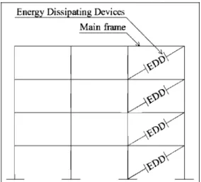
A typical building structure with passive control sys-tems consists of a main frame designed for sustaining mainly the gravity loads and a series of special energy dissipating devices (EDDs), also called dampers, whose main role is to dissipate most of the energy input by the earthquake, as shown in Figure 1. Several mechanisms have been used as EDDs for passive energy dissipation, including metal yielding, phase transformation of metals, friction sliding, fluid orificing, and deformation of viscoelastic solids or liquids.7 9 Among the different EDDs for passive control of structures, the so-called hysteretic damper is one of the most widely used. The source of energy dissipation in hysteretic dampers is the plastic deformation of metals (commonly steel), for which reason they are also known as metallic dampers.

When designing structures with this type of EDD, the connection of the element to the rest of the structure is designed so that it remains elastic (with no damage) for the maximum feasible force that can be sustained by the damper itself; therefore, the damage in the connec-tion is not a concern. However, because inelastic strains in the material involve damage, evaluating the health of the hysteretic damper after a seismic event is a matter of great concern. Furthermore, the same geometry and type of steel is used for all the EDDs (I-section steel seg-ments) installed in the buildings. The lateral strength required in each story is adjusted by varying the

Energy Dissipating Devices Main frame

4 ^

^

^

Figure I. Basic configuration of a structure with energy

dissipating devices.

number of I-section steel segments, but not the charac-teristics of the I-section steel segment.

For minor or moderate earthquakes (with a prob-ability of exceedance of 50 %> and 20 %>, respectively, in 50 years), the main frame of a structure with hysteretic dampers is commonly designed to remain within the elastic range (i.e. undamaged), and most of the seismic energy input by the earthquake is assumed to be dissi-pated through plastic deformations on the hysteretic dampers. Minor to moderate earthquakes can occur several times during the lifetime of the structure and usually do not exhaust the energy dissipation capacity of the hysteretic dampers, though they do cause dam-age. Hysteretic dampers may be effective even after a major earthquake because their ultimate energy dissipa-tion capacity is commonly very large. Hysteretic EDDs need not be replaced after a minor/moderate or even after a large earthquake provided that their health (level of damage) can be reliably evaluated. Such evaluation cannot be based on simple visual inspection because the damage caused by the plastic deformation of the steel is not visible until the element is on the brim of failure.

Past research10 has shown that the level of damage and the proximity to failure of steel components sub-jected to arbitrarily applied cyclic loading (such as that

imposed by earthquakes) can be reliably estimated by decomposing the force-displacement curve experienced by the metallic damper in the so-called skeleton and Bauschinger parts through an index of damage (ID). The skeleton part is formed by sequentially connecting the segments of the axial force-axial deformation curve of the damper that exceed the load level attained by the preceding cycle in the same domain of loading. The remaining part of the curve is called the Bauschinger part. The ID depends on the plastic strain energy dissi-pated in the skeleton and in the Bauschinger parts.

However, measuring the force and the displacement of the hysteretic damper during an earthquake entails installing expensive instrumentation (load cells or strain gages, displacement transducers, etc.) on the dampers. This reduces one of the main advantages of hysteretic dampers, low cost, and would not be justified for a type of action, earthquake, whose probability of occurrence is very low. Alternatively, the use of piezoceramic sen-sors permanently attached to the hysteretic damper pro-vides a preferable (cheaper) solution for instrumenting the EDDs and allows for conducting simple vibration tests to evaluate the level of damage using structural health monitoring (SHM) strategies. Piezoceramic sen-sors are low-cost devices that can be used both to excite the dampers and to measure their response.

in the context of seismic control systems such as dam-pers. Research in this area involves numerical simula-tions of the response of a building model equipped with dampers and excited by means of dynamic sig-nals,4'5 whereas few studies compare the numerical simulation results with real experimental outcomes.

Vibration-based damage detection strategies are based on the correlation between the vibration response of the structure and the presence of damage.21'22 Damage alters the vibration response of the structure (resonance frequencies, modes, damping coefficients, etc.), and this can be detected and evaluated by ade-quate processing of signals captured by the sensors and correlated with the presence (Level 1 in SHM), position (Level 2 in SHM), and intensity of damage (Level 3 in SHM).

A number of research studies deal with time vibra-tion series analysis for damage detecvibra-tion in structures and materials (such as buildings, airplanes, and compo-sites).21 23 Most of these algorithms use natural fre-quencies as damage indicators. The principal advantages of frequency measurements are that signals can be quickly acquired24 and that brief damage detec-tion methods can be implemented. Some of these meth-ods are based on frequency response functions (FRFs). FRF-based methods are feasible indicators of struc-tural damage and can obtain damage information from in situ measurements without an exhaustive modal analysis. F R F methods are straightforward25 and do not require many sensors to provide reliable informa-tion about the structural dynamic behaviour.26 Also, novel studies on structural diagnosis combine F R F with soft computing techniques27 29 to obtain enhanced results.

Research on the FRF-based method for damage detection may use direct measurement of FRF,3 0 F R F curvatures,31 FRF differences,28 or compressed FRFs,2 7 but thus far, none of these techniques has been applied to evaluate the level of damage on hysteretic dampers through comparison or correlation with mechanical indexes of damage.

This article presents an experimental investigation on a practical SHM system proposed for a particular type of hysteretic EDD that consists of short segments of I-shaped steel sections whose source of energy dissi-pation is the plastification of the web. Four I-section steel segments were instrumented with piezoceramic sensors and subjected to the same pattern of cyclic load-ing. The applied force and the corresponding displace-ment were continuously recorded. At several stages of the cyclic loading, corresponding to different levels of damage referred to as Dt hereafter, the cyclic loading

was stopped, and the I-section steel segments were sub-jected to controlled white noise random vibrations. In these vibration tests, the web of the I-section was

excited with a piezoceramic actuator attached to one side of the web, and the signal was recorded by a piezo-ceramic sensor attached to the opposite side. The load-displacement curve recorded up to the point where the cyclic loading stopped was decomposed to calculate an energy-based ID. Also, the signals recorded with the vibration tests conducted after each interruption of the cyclic loading were analyzed using a nonparametric FRF-based method.21 From these analyses, a new ID called area index damage (AID) was defined. A good correlation is found between ID and AID, and this indi-cates that the level of damage on the hysteretic EDD can be readily estimated from simple vibration tests, with no need to know the load-displacement relation-ship and without resorting to cumbersome and expen-sive instrumentation.

Description of hysteretic E D D s

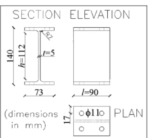
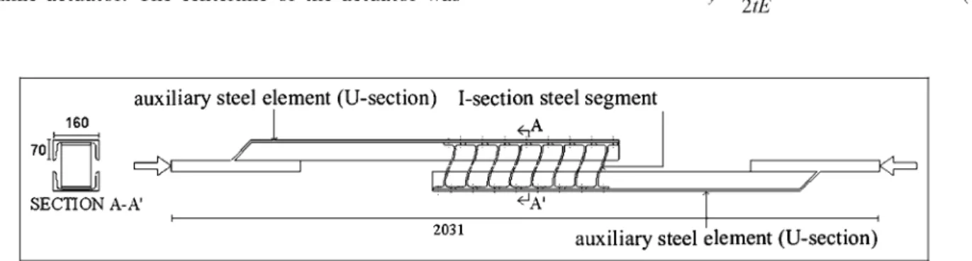
The hysteretic EDD investigated in this study consists of I-section steel segments that are assembled and installed in the structural frame in such a way that the energy is dissipated through out-of-plane plastic strains on the web of the I-section when the frame is subjected to lateral seismic loads.32 Figure 2 shows the typical I-section steel segment that constitutes the hysteretic EDD itself. Figure 3 shows its deformation pattern, the shaded region indicates the locations where plastic deformations occur. Figure 4 shows a simple solution for assembling the EDDs to form a structural member that can be installed in a frame as a conventional brace. This assemblage uses auxiliary steel elements called U-sections that are designed to remain elastic, while the I-section steel segments undergo plastic deformations. The details on the dimension of U-sections are pro-vided in Figure 4.

SECTION ELEVATION

O —

-s:

t=5

73

(d m e n s i o n s

/=90 0(|>ll0

o o

PLAN

Figure 2. Hysteretic EDD: nominal dimensions of test

Figure 3. Deformation pattern of the EDD.

E x p e r i m e n t a l investigation

Test specimens and experimental setup

From a hot-rolled I-section steel profile, four short seg-ments of identical length were cut to constitute the EDDs (test specimens) investigated in this study. They will hereafter be referred to as specimens II through 14. The nominal geometry of each specimen is shown in Figure 2. The specimens were mounted in the setup shown in Figure 5. The flanges of the test specimen were fastened to two U-shaped sections by post-tensioning four high-strength bolts with a torque of 67 Nm each. One of the U-sections was securely fastened to a stiff reaction wall, while the other was connected through a pin-joint to an MTS 250 kN capacity dynamic actuator. The centerline of the actuator was

contained in the horizontal plane of symmetry of the test specimen. The piston of the actuator was allowed to displace in the horizontal direction. A counterweight was installed to avoid the self-weight of the testing apparatus from loading the test specimen. A load cell installed between the actuator and the pin-joint mea-sured the horizontal restoring force V opposed by the specimen when subjected to forced cyclic displace-ments. A displacement transducer connecting the upper flange of the I-section and the reaction wall provided the relative horizontal displacement 8 between the upper and lower flanges of the test specimen.

Cyclic tests: instrumentation and loading history

Horizontal relative displacements were imposed with the actuator between the flanges of the I-section steel segments using the setup shown in Figure 5. The load-ing pattern consisted of successive cycles of increasload-ing displacement amplitude, as shown in Figure 6, follow-ing the sequence 58 y, 108y, 158y, 208y, 258y, and 305-,,.

Here, 8y (= 1.5 mm) is the horizontal yield

displace-ment of the specimen32 calculated with equation (1)

' 2tE (1)

1-70l|/

160

SECTIO

auxiliary steel element (U-section) I-section steel segment

I . . . < A . . .

II ^ -/ , TTTTTTl-P

NA-A' ^A'

' 7 K x^

2031 auxiliary steel element (U-section)

Figure 4. Assemblage of EDDs to form a brace-type structural member showing the main parts: I-section and U-section

(dimensions in millimeter).

Counterweight

v l

Hydraulic actuator

XI

Load cell

Displacement transducer

Pin connection Test specimen.

£=

Figure 6. Loading history.

where fy is the yield stress of the steel, E is its modulus

of elasticity, and h and t are the height and web thick-ness of the I-section steel segment, respectively, as shown in Figure 2. The corresponding yield strength Vy

of the EDDs can also be estimated as follows32

Vv lt%

2h (2)

Here, the new parameter / is the length of the steel seg-ment as shown in Figure 2. The cyclic rate applied by the actuator was 1/80 Hz. The qualitative level of dam-age attained by a given specimen after i cycles of load-ing is referred to as D{ in the horizontal axis of Figure

6. DQ represents the initial undamaged state. Specimen

II was subjected to five cycles and specimens 12,13, and 14 to six cycles of displacement.

Vibration tests: instrumentation, applied signal, and preprocessing

Before applying the cyclic loading on the test specimen, that is, when the level of damage was DQ, and at

inter-mediate and/or final levels of damage Dh the specimens

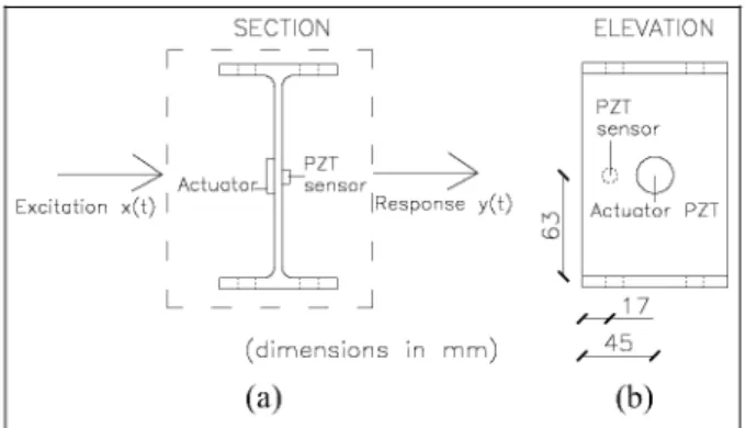
were subjected to vibration tests. For specimens II and 12, vibration tests were conducted only at the end of the cyclic test, while for specimens 13 and 14, vibration tests were carried out at the end of each cycle to investigate the progress of damage. To conduct the vibration tests, the web of the specimen was instrumented with one piezoelectric ceramic (lead zirconate titanate (PZT)) sensor glued on one side and another PZT sensor glued on the opposite side at the location shown in Figure 7. The location of the PZTs was determined using the cri-terion of separating the PZT from the regions of largest plastic deformation in order to avoid damaging the PZT. In the EDDs under study, maximum plastic strain areas were expected at both ends of the web of the I-sec-tion (see Figure 3), while strains at the center of the web are nominally zero. Therefore, the PZTs were placed at the center of the web of the I-section.

The vibration tests consisted of exciting the web of the I-section by means of a controlled vibration signal

x[t] applied at the PZT on one side of the web

SECTION ELEVATION

Excitation x(t) I :tuatop-|_

PZT sensor

>-„,

iResponse y(t) Actuator PZT

.17 (dimensions in mm) / /

(a) (b)

Figure 7. Position of sensors on specimen: (a) section view

and (b) frontal view. PZT: lead zirconate titanate.

("actuator" in Figure 7) and recording simultaneously the response at the PZT located on the opposite side ("sensor" in Figure 7). The signal recorded by the sen-sor is referred to as y[t] hereafter. The PZT used as actuator was a PI®PRYY 0842. The PZT used as sen-sor was a PI®PRYY 0220. The signals y[t] recorded with the PZT sensor had a voltage amplitude of about 3Vp.

Bruel & Kjeer PULSE equipment was used as signal generator of the random excitation x[t] and as acquisi-tion system to record the response vibraacquisi-tion signals y[t]. The PULSE system provides an output signal with a maximum peak at about 5 V, which was seen to be insufficient to properly excite the specimen. Therefore, a gain G = 20 was used. In addition, to ensure good quality of the signals, the acquisition system was config-ured in the differential mode. This configuration made it possible to measure the signal of each PZT as the dif-ference between the two channels, thus avoiding any reference to the electric ground. Moreover, to avoid both mechanical and electric noise, a ground system was installed throughout the cable network and con-nected to an embedded mass system that was indepen-dent of the ground system of the laboratory building.

For both x[t] and y[t] signals, the sampling frequency used was fs = 65,536 Hz, which corresponds to a sam-pling period of At = 1.5 X 10~5 s. The total number N of data recorded was N = 657,408, corresponding to 10 s of acquisition time. For statistical reasons, five vibra-tion tests were carried out for each level of damage Dt

and for each specimen, using a different white noise sequence in each but maintaining the same frequency content and variance. The signals recorded during the vibration tests were suitably preprocessed for data con-ditioning purposes. This preprocessing consisted of the following steps:

Table I. Eigenfrequencies (kHz) of the undamaged specimens.

Test specimen

Mode 1 Mode 2 Mode 3 Mode 4

II

1.56 4.57 9.56 23.93

12

1.58 4.59 9.58 24.04

13

1.59 4.57 9.50 23.91

14

1.57 4.59 9.57 23.95

and avoid nonlinear performance of the sensors. Finite element numerical simulations conducted prior to the tests confirmed that at least 17 eigen-frequencies of the test specimen were located inside the frequency BW of 0.3-25 kHz. This BW was considered sufficient for damage detection and eva-luation purposes. It is worth noting that although the four specimens were cut from the same profile, due to the hot rolling process, tolerances up to about ±10% from the nominal size can be expected. Because of these variations on the nom-inal geometry, the eigenfrequencies of the four spe-cimens before applying any damage were slightly different. Table 1 shows the values of four relevant eigenfrequencies used in this study for health moni-toring purposes, as explained later.

2. Normalization and scaling. Due to numerical rea-sons, in order to counteract different excitation lev-els and environmental conditions and in order to compensate the offset and amplitude variability among the signals, the following normalization process was applied

x[t -x[t y[t -y[t n,

x M

»

=

^r

; j M

»=^r

(3)

where x[t]n and y[t]n are the normalized signals, x[t] and y[t] are their mean values, and <T(X) and a(y) are their

standard deviation, respectively. For the sake of clarity, from now on, the sub-index n will be removed and the simpler notations x[t] and y[t] will be used for the nor-malized signals instead of x[t]n and y[t]n, that is, x[t] =x[t]n and y[t] =y[t]„. Thus, after acquisition and signal

conditioning, vibration data recorded for each speci-men were collected in a vector denoted as z[t] = [x[t],

y[t]f-Mechanical damage evaluation f r o m t h e V-S curves through index / D ;

Decomposition of the V-S curves

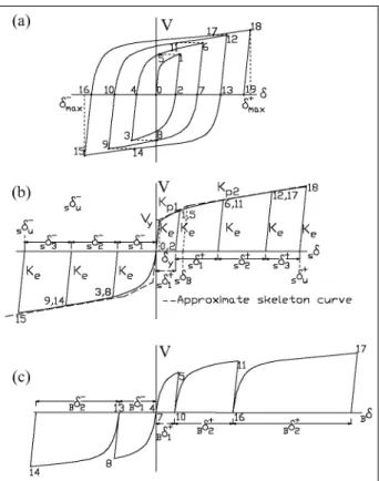
Figure 8(a) shows the typical load-displacement rela-tionship, V-8, obtained from the cyclic tests. The V-8 curve exhibited by the test specimen up to a given level

Figure 8. Decomposition of a typical V-8 curve: (a) initial V-8

curve, (b) skeleton part, and (c) Bauschinger part.

of damage Dt defined by point i of the coordinates (ViSi) can be decomposed into the so-called skeleton

part and the Bauschinger part as shown in Figure 8(b) and (c), respectively. The skeleton part (Figure 8(b)) is derived by sequentially connecting the segments 0 1 , 5 -6, 11-12, and 17-18 in the positive domain and 2-3, 8-9, and 14—15 in the negative domain—these being the paths that exceed the load level attained by the preced-ing cycle in the same domain of loadpreced-ing. Segments 1-2, 6-7, 12-13, 18-19, 3-4, 9-10, and 15-16 are the unload-ing paths, whose slope coincides with the initial elastic stiffness Ke( = Vy/8y). For each domain of loading, the

area enveloped by the skeleton curve up to a given point

(Vit Si) will be called sWf and SW^. The segments 4-5,

10-11, and 16-17 in the positive domain and 7-8 and 13-14 in the negative domain of loading—which begins at V = 0 and terminates at the maximum load level pre-viously attained in preceding cycles in the same loading domain—are the so-called Bauschinger part (Figure 8(c)). For each domain of loading, the sum of the areas enveloped by the Bauschinger part up to a given point

(Vit S^ will be referred to as sWf and ^W^. The sum sWf +BW^ in the positive domain, and sWf +BW^ in

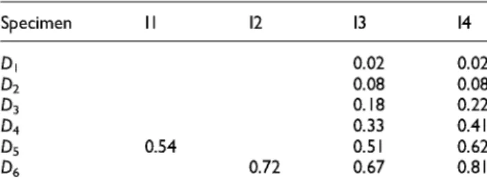
Table 2. Value of the index of damage.

Specimen 14

D, D2

D3

D4

D5

D6

0.54

0.72

0.02 0.08 0.18 0.33 0.51 0.67

0.02 0.08 0.22 0.41 0.62 0.81

nondimensional form in terms of the new ratios 517,+ ,

fi{~, s^k , and rjj~ defined as follows

sVt

sVt

VyOy

Wi

Vy8y

vysy vysy

(4)

Evaluation of mechanical damage through an energy-based index ID

Past research10 showed that the level of mechanical damage in a metallic EDD subjected to arbitrarily applied cyclic loading up to a point i (Vt, 8,) can be

accurately predicted using the following index

specimen is considered to be undamaged (S0) and the

opposite hypothesis, H\, under which the inspected spe-cimen is considered to be damaged. Such conditions are mathematically expressed as follows21

H0 : SU = S0 : null hypothesis (undamaged specimen)

(7)

H\ : Su=£ S„ : alternative hypothesis (damaged specimen)

(8) The decision between hypotheses H0 and H\ is taken on

the basis of a quantitative parameter called characteristic quantity Q along with some statistical considerations.

The statistical time series method for damage detec-tion entails three phases.21 The first phase, called the baseline phase, consists of data acquisition and statisti-cal modeling of the undamaged specimen S0; in this

phase, from the vibration response data, z0[t], the

esti-mation of characteristic quantity Q0 is made. In the

second phase, the inspection phase, the characteristic quantity Qu is estimated from the vibration response

data, zu[t], of the inspected structure Su. Finally, the

statistical decision-making phase (equations (7) and (8)) consists of comparing Qu and Q0 by means of

sta-tistical tests. A general scheme is offered in Figure 9.

ID, = max{ID, , ID,. } where

ID:

(5)

(6)

In equation (6), fj+ and fj~ represent the ultimate energy dissipation capacity of the EDD, which depends on the values of sr]f, rtf, ST)J, and r]J and on the two

empirical parameters a and b related to the material properties of the steel and the geometry of the EDD. A detailed explanation of these parameters and their value for the type of EDD investigated in this study can be found in Benavent-Climent et al.32 The value

IDt = 0 indicates no damage, while IDt = 1 means

complete failure. The values of the mechanical index of damage IDt calculated for the damage levels D1 ; D2, D3, D4, D5, and D6 according to Benavent-Climent et

al.32 are summarized in Table 2.

D a m a g e assessment by processing vibration test results: AID index

Level 1 in SHM is used to ascertain whether the inspected specimen, named Su hereafter, has damage or

not. At this stage, a decision must be made between two options: hypothesis H0, under which the inspected

FRF-based method for damage detection and statistical test

Past research33 showed that the F R F is a good method to detect the presence of damage on the EDD investi-gated; it is used in this study as the characteristic quan-tity Q. The FRF-based method uses both excitation x[t] and response signals y[t], and its physical basis is the detection of changes in the frequency response of the specimen when damage appears, that is, damage detec-tion is based on confirmadetec-tion of statistically significant deviations (from the healthy S0) in the inspected

speci-men F R F at some frequencies.21

The magnitude of FRF, \H(Jco) \, is calculated as

OF \H(j(o)\

\Sxy(Jco)\

Sx(<w)

(9)

where |5XJ,(/'<w)| and |5x(<w)| are the cross and auto-spectral density functions, respectively, estimated via the Welch method.34

This estimator of the FRF, \H(Jco)\, has an approxi-mately normal distribution with mean the true FRF,

\H{jco)\, and variance, cr2(<w), as is demonstrated in Bendat and Piersol,35 that is

\H(jco)\~N(\H(jco)\,cr2(co))

where the variance is given by

Baseline phase

Data acquisition

structure S,

WY

responses

JUT

Data preprocessing *<>['] >'<>[']

- filtering - normalization

Obtain data

-»['] = [*.[<]•>'»[']]'

Estimation of Q -»['] ,>'»[']

FRF

tf-C/V) Non-paramedic model

QP healthy structure

Inspection phase

Data acquisition

structure S„

m

-0-responses

m

Data preprocessing *»M yAt] - filtering - normalization

Obtain data

--,,['] = IM'UiMf

Estimation of Q _--M yM

FRF

H„Vw)

Non-parametric model

ted str inspected structure

statistical decision

H, : S„ = S0

or

H\ : S„ + S0

Qu

F i g u r e 9 . General scheme o f t h e statistical t i m e series methods f o r damage detection. FRF: frequency response function.

a1 {a>y 1 _{y 2 M}

l ^ ) l

y2(co)2K (11)

K being the number of segments in which the used data

are divided, and

r

M

Sx(o))SY((o) (12)

the coherence function.21

Thus, the algorithm to detect the damage based on the F R F estimator can be summarized in the follow steps.21'33

Obtain the characteristic quantity Qufor the inspec-tion structure: in the same way, Qu is calculated

with equation (9) using the available data zu[t] to

estimate the magnitude \Hu(Jco)\.

Set up the statistical hypothesis-testing problem for fault detection: the hypothesis test is configured

using the characteristic quantity selected and fol-lowing equations (7) and (8). In this case, the hypothesis test is formulated as

Ho : \H0(jaj)\ H\ : \H0{jco)\

\Hu(jaj)\=0

\Hu{jco)\^0 (13)

1. Obtain the characteristic quantity Q0for the healthy structure: this quantity is calculated following

equa-tion (9) using the available data za[t] to estimate the

magnitude \H0(Jco)\.

S\H{jco)\ = \H0{jco)\ - \Hu{jco)\ (14) points

Note that since \H0{j<a)\ and \Hu(Jco)\ are independent

normal variables, the difference has a distribution with mean 8 \H(Jco) | and variance 8a2 (<w), that is

8\H{jw)\~N{8\H{jw)\,8(T2{w)) (15) H0(jco)\ - \Hu(jco)\ and 8a2(co) = a20

where 8 \H(ja>)

{co)+a2(co).

Evaluate the statistic under the null hypothesis:

under H0 (equation (13)), it is assumed that the

inspection specimen is healthy, the two real magni-tudes are the same \H0(Jco)\ = \Hu(Jco)\, and the

var-iances are the same as (r20{(a) = cr2,(<w). Then, the distribution of 8\H(Jco)\ (equation (15)) can be written as

8\H(joj)\~N(0,2cro2(w)) (16)

6. For convenience, the statistic is normalized to have a standard normal distribution, that is

z=

pp

-

mi)

V 2cr0 M

(17)

where &20{(a) is the variance of F R F estimated for the

undamaged specimen in the baseline phase.21

As long as Zaj1^Z^Z\_aj1, that is, the Z-statistic

remains within the confidence interval, the null hypoth-esis H0 will be accepted and the inspected specimen will

be considered undamaged. Otherwise, if the inequation is not satisfied, the hypothesis H\ will be accepted and the specimen will be considered as damaged, a deter-mines the probability of false alarm and is called risk

level, whereas Zan and Z\_an are called the critical

21,36

Damage estimation: definition of damage index AID

In Figure 10, the |Z|-statistic is plotted against the fre-quency. If the entire |Z|-statistic plot is under the criti-cal point (dashed horizontal line at level |Z| =Z1_a/2) m Figure 10(a), the inspected specimen is assumed to be undamaged with the level of certainty associated with

a. Otherwise, if some peaks of the |Z|-statistic cross the

critical point (Figure 10(b)), the inspected specimen is considered damaged.36

Previous experiments33 on the type of EDD investigated showed that when the magnitude of damage increases, the area of |Z|-statistic increases pro-portionally in some frequencies sensitive to damage. Thus, an AID was proposed to estimate the intensity of the damage (Level 3 in SHM) following this equation

AID-- \z((o)\, yz((o)>Zi_ a/2 (18)

Analysis of signals obtained from vibration tests and calculation of AID

Figure 11 shows the magnitude of F R F spectra esti-mated from vibration response signals y[t] of one of the specimens (14) for each level of damage, that is, from

DQ to D6, in the whole BW of [0.3-25] kHz (for clarity,

the full BW has been divided into five separate graphs of 5 kHz wide).

The following parameters to estimate the Welch-based F R F were used: (1) 128,000 sample windows; (2) number segments, K = 5, without overlapping; and (3) frequency resolution of the F R F estimated = 0.512 Hz. In Figure 11, four regions of the spectra, namely, BW1,

-10

£• "20

T3,

a>

"D

.•3 -30

c

D ) CC 2

^ 0

-50

-60

-70

-12

-14

-16

-18

£"

V -20 I -22

2

-24

-26

-28

-30

1 1

(b)

-~ ^ ^ ^ = 4

" • ^s* * a c = E£-= 3«

-i -i

i i i

!:

i i i

i

t\i

Ml

i

f

-1

1 1

« 1

J\ In

AN TJ

*w

BW3

1 *

1

f

- D , _ D2 D3— - D4_ D5— - [

i i i

-~~

'

_

M

5.5 6.5 7 7.5

Frequency (kHz)

8.5 9.5 10

-i i i

1 (

; '

w 1 1

1

i i

i i i

!

| D0_ D , D2 D3 D4

-i -i -i

1

w '

V

-- D5— - D j i

10 10.5 11 11.5 12 12.5 13

Frequency (kHz)

13.5 14 14.5 15

17 17.5 M Frequency (kHz)

18.5 19 19.5 20

20

15

10

5

2 0

CD

i -5

c cc 2 -10

-15

-20

-25

-30

-

(e)

I I

I

I

I

0%

A

wf

- V

I

I

/

A i^

#

I

I

i

i i i

; j _ C&£^

^^S^sSSS^-^V'

— I 1 1

A , BW4

i' jWJm

I //•;*, W m i l i \ i

-^

-| _ D0 D , _ D2 D3_ D4 D5-— D6|

i i i i i i

20 20.5 21 21.5 22 22.5 23

Frequency (kHz)

23.5 24 24.5 25

F i g u r e I I . Magnitude o f FRF spectra estimated f o r specimen 14 o n bandwidth (a) [ 0 - 5 ] , (b) [5— 10], (c) [ I 0 - I 5 ] , (d) [ 1 5 - 2 0 ] , and (e) [ 2 0 - 2 5 ] k H z f o r all levels o f damage (bandwidths sensitive t o damage are highlighted in rectangular b o x in (a), (b), and (e); no bandwidths sensitive t o damage are selected in (c) and (d)).

BW: bandwidth.

BW2, BW3, and BW4, which are considered more sen-sitive to damage, are given in the rectangular box. The selection of these regions was made on the basis of pre-vious finite element calculations, which indicated that the shape of the vibration modes associated with these frequency ranges provided the largest displacements at the location of the PZTs.

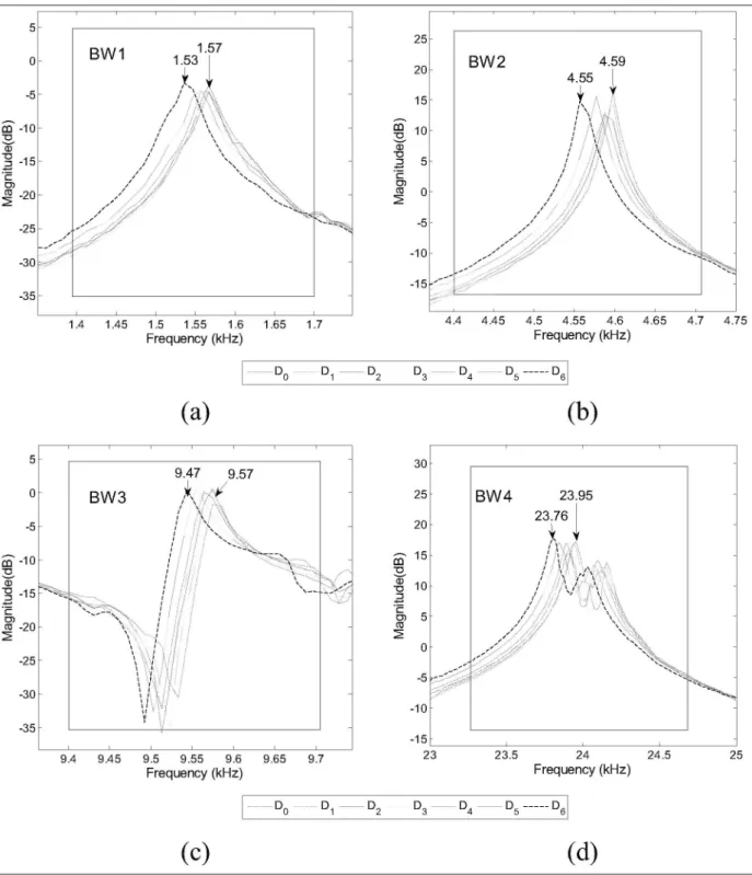
The BWs of these enclosed areas are as follows: BW1 = [1.4-1.7], BW2 = [4.4-4.7], BW3 = [9.4-9.7], and BW4 = [23.4-24.7] kHz. Figure 12 shows zooms of these frequency BWs, where a clear shift of the

frequency response can be observed, which clearly increases with the level of damage.

It can be seen that the total frequency shift from the undamaged structure, DQ, to damage level D6 is

5 0 -5 m -10 T3 01 R-15 g n J -20 -25 -30 -35 -y -**-*>' BW1 J / / ••'

/''//S

i

/

\ ,

/ 7 ^ Vl"

/if K~- \ \

'I

^ 3 \

^S.

1.4 1.45 1.5 1.55 1.6 1.65 1.7

Frequency (kHz)

(a)

9.4 9.45 9.5 9.55 9.6 9.65 9.7

Frequency (kHz)

(c)

25

20

15

3

01 T3 3 5 c CD tB 0 2 -5 -10

-15 _*'~

BW2 / /'' --''-^ -;:-.' ' 4.59 4.55 I

it

/ m \w

< 1 / & \ \ \ \ / .• / :• \ \ •• V

-/ . • ' • -/ -/ • \ \ ' ' . \ \ //#' \ ' • • .

f

v^

-3SSS,

-%,

^ ^ s

-4.4 -4.45 4.5 4.55 4.6 4.65 4.7 4.75

Frequency (kHz)

(b)

1 V

\ 1

?

9.47 9.57

A A

' / / / • / ''''''''•--""i'i';t-;--^\

/ / / / / / Sv"

' /' " " -CD 5 CD -15 23 _^> BW4 / //

- V

i 1

' .• ' . \ / v

v^ o \

^ V

-^ " • x *

-23.5 24 24.5

Frequency (kHz)

25

(d)

Figure 12. Details of four bandwidths sensitive to damage selected from the magnitude of FRF spectra estimated in specimen 14

for the levels of damage D0,Dh D2, D3, D4, Ds> and D6: (a) BWI = [ 1.4-1.7] kHz, (b) BW2 = [4.4^.7] kHz, (c) BW3 = [9.4-9.7]

kHz, and (d) BW4 = [23.4-24.7] kHz. BW: bandwidth.

5 o 4

.52 3

CO "GO 2

zl

4

°i

X.

4 4.5 4.6

kHz

5 1 — — • — — • —

0 4

1 3

.2

"GO 2

Z

l

o

4

D4

All

_ylL

4 4.5 4.6

kHz

5

O 4

•£ 3

CD "GO 2

^ 1

4 7 %

D?

i

i

kHz

4

0 4

1 3

.2

"GO 2

FT

1

7 1/

• °6

•

_y

_V

4 4.5 4.6

kHz

.

4.7

4.7

5

O 4

.52 ? CD

CO 2

^ 1

2

D3

1

A

4 4.5 4.6

kHz

5

0 4

1 3

.2

"GO 2

FT

8

n°

4 4.5 4.6

kHz

4.7

4.7

Figure 13. Application of the FRF-based statistical test to different levels of damage for the specimen 14 and BW2 = [4.4—4.7] kHz.

For the four specimens tested, Table 3 summarizes the values of the index AID calculated in each BW and level of damage Dp As seen in Table 3, the range of val-ues of AID varies depending on the frequency band considered. The range is similar for BW1, BW2, and BW3 (between approximately 25 and 300) but increases notably for BW4 (between 230 and 1300). This means that the highest frequency band is most sensitive to damage. It is also worth noting that the values of index AID for the same level of damage Dt (and especially

for D6) are similar among the four specimens, which

indicates that the technique applied to the EDDs is robust.

In order to give an idea of how the group data from different tests are dispersed, Figure 14 shows an analysis of the dispersion of the AID for the specimen 14 and the four frequency bands and the six levels of damage used. The whiskers, in black color, show the maximum and minimum values obtained for AID in each test, and the boxes have lines at the median, lower, and upper quartile values. We can clearly appreciate the stability of the results against the ran-dom noise used as excitation of the healthy and inspected specimens. In general, the dispersion is small and has little influence on the results and its sta-bility. This fact supports the validity and usefulness of the correlation given by equations (19) and (20) proposed in the next section.

Correlation between the indexes ID and A I D : prediction of ID from A I D

In Figure 15, the index AID is represented against the ID for the four frequency ranges investigated. It is clear from the figures that the relation between AID and ID for the four specimens in each frequency band can be approximated by a single curve/line. This means that the AID-ID relationship follows a clear and common pattern irrespective of the specimen considered.

Except in the lowest frequency range, in which the relation between AID and ID follows an approximately logarithmic law, in all the other frequency ranges, the relation between AID and ID is clearly linear and can be approximated by the following equations

Frequency ranges [4.4 — 4.7] and [9.4 — 9.7] kHz :

ID = 0.0035 AID= - 0 . 2 5 (19)

Frequency range [23.4 — 24.7] kHz :

ID = 0.00075, AID= - 0 . 2 0 (20) Comparing Figure 15(b) to (d), it is clear that the fit

T a b l e 3. Value of index A I D .

Bandwidth (kHz) Specimen damage level 12 13 14

BWI =[1.4-1.7]

BW2 = [4.4^.7]

BW3 = [9.4-9.7]

BW4 = [23.4-24.7]

D, D2 D3 D4 D5 D6 D, D2 D3 D4 D5 D6 D, D2 D3 D4 D5 D6 D, D2 D3 D4 D5 D« 107.05 281.83 155.15 309.62 189.32 278.49 906.06 1409.00 49.49 48.72 50.58 63.34 1 16.05 266.21 62.69 86.92 109.86 157.65 217.04 295.35 1 18.70 86.52 128.89 163.55 207.90 273.63 297.77 390.22 449.57 658.97 932.45 1291.78 25.81 36.05 38.58 71.47 150.17 321.38 34.13 68.36 85.09 1 16.07 212.98 287.94 72.37 II 1.68 126.75 157.47 236.62 312.64 237.16 503.03 543.27 777.45 1051.62 1285.76 300 250 200 150 100 50

D1 D2

300 250 9 200 < 150 100

D1 D2

I 4 B W 1

D3 D4 Damage level

I 4 B W 3

D5 D6

D3 D4 Damage level

D5 D6

300 250 200 Q < 150 100

50 ^—

I4BW2 — ^ = = '

-D1 D2 D3 D4 Damage level

D5

D1 D2 D3 D4 Damage level D5 D6 1200 1000 Q 800 < 600 400

200 . =

= I4BW4 — ^ _ =sss^ -= -D6

F i g u r e 14. Value o f t h e A I D f o r all t h e tests on specimen 14. The whiskers, in black color, s h o w t h e m a x i m u m and m i n i m u m values obtained f o r A I D in each test. T h e boxes have lines at t h e median, lower, and upper quartile values.

(a)

1.0

ID

A Specimen 2 • Specimen 1

• Specimen 4 + Specimen 3

(b)

(c)

1.0

0.8

0.6

0.4

0.2

0.0 0

1 0

0 6

0 4

0 . 2

-0.0

ID

50 100 150 200 250 300 350

(d)

ID

- ^ - Specimen 3 ^ Specimen 4 H Specimen 1 A Specimen 2

0.8

0.6

0.4

0 2

JST ID=0.0035AID-0.25

AID

-Specimen 3 — [ ^ S p e c i m e n 4 • Specimen 1 A Specimen 2

>

-ID=0.0035AID-0.25

AID

50 100 150 200 250 300 350

ID

0 Specimen 3 — i > - Specimen 4 I ] Specimen 1 A Specimen 2

/ ' / ID=0.00075AID-0.20

AID

50 100 150 200 250 300 350 250 500 750 1000 1250 1500 1750

F i g u r e 15. Comparison between A I D and ID in different frequency bands: (a) B W I : 1.4-1.7 kHz, (b) B W 2 : 4.4-4.7 kHz, (c) B W 3 : 9.4-9.7 kHz, and (d) BW4: 23.4-24.7 kHz.

AID: area index damage; ID: index of damage; BW: bandwidth.

monitor the damage on the EDDs under study. Once the index AID is calculated in this range, the corre-sponding index of mechanical damage ID can be read-ily obtained with equation (20).

Finally, in a real structure, the EDDs should be replaced when the damage quantified with the index ID and calculated from simple vibration tests with equa-tions (19) and (20) approaches ID = 1 (a reasonable limiting value would be ID = 0.75). These vibration tests should be conducted after an earthquake or strong wind storm.

Conclusion

In this experimental study, a health monitoring tech-nique to quantitatively evaluate the damage in hystere-tic dampers subjected to cyclic loading is investigated. The type of damper under study consists of a segment of I-section steel profile. The technique uses nonpara-metric statistical processing of the excitation and response signals obtained from simple vibration tests

conducted with two piezoelectric ceramic sensors glued to the web of the I-section.

Acknowledgements

The authors appreciate the collaboration of Andres Roldan-Aranda for his help in the experimental setup.

Declaration of conflicting interests

The authors declare that there is no conflict of interest.

Funding

This research received the financial support of the local gov-ernment of Spain, Consejeria de Innovacion, Ciencia y