A mathematical framework for new fault detection schemes in nonlinear stochastic continuous-time dynamical systems

A mathematical framework for new fault detection schemes

in nonlinear stochastic continuous-time dynamical systems

Pedro J. Zufiria

A B S T R A C T

In this work, a mathematical unifying framework for designing new fault detection schemes in nonlinear stochastic continuous-time dynamical systems is developed. These schemes are based on a stochastic process, called the residual, which reflects the system behavior and whose changes are to be detected. A quickest detection scheme for the resid-ual is proposed, which is based on the computed likelihood ratios for time-varying statis-tical changes in the Ornstein-Uhlenbeck process. Several expressions are provided, depending on a priori knowledge of the fault, which can be employed in a proposed CUSUM-type approximated scheme. This general setting gathers different existing fault detection schemes within a unifying framework, and allows for the definition of new ones. A comparative simulation example illustrates the behavior of the proposed schemes.

1. Introduction

Model-based schemes for dynamical system fault detection make use of an explicit analytical system representation for redundancy checking, so that they generate the residual as a measure of discrepancy between the model and real system behavior. Residual generation and analysis techniques have been extensively developed in two directions. On the one hand, stochastic discrete-time models combine statistical hypothesis tests with geometrical tools in the design and characteriza-tion of deteccharacteriza-tion algorithms for linear systems [5,15,20,23]. On the other hand, deterministic continuous-time models, which make use of identification and control theory tools, have shown to be suitable for nonlinear system fault detection [1,15,17,19,46,47,60].

Recently, continuous-time nonlinear stochastic models have been employed in system fault diagnosis [12,13,41-43,50]. These models can characterize system and sensor noises as well as disturbances in very elegant and analytically concise for-mulations; in addition, they can exploit the advantages of statistical tools for evaluating the quality of the detection schemes. These new detection and isolation proposed algorithms are based on the generation of a residual modelled as a continuous-time stochastic process. The residual known statistics under the no-fault hypothesis, do change when a fault occurs; hence, these schemes rely on the detection of statistical changes in such residual stochastic process.

The paper is organized as follows. In Section 2, the design of system fault detection schemes is presented as a residual change detection problem. The steps proposed for a quickest detection scheme are presented in Section 3. Different log-like-lihood ratios are computed in Section 4 and new CUSUM-type approximated algorithms are proposed in Section 5. A com-parative simulation example is developed in Section 6 to illustrate the theory. Finally, some concluding remarks are summarized in Section 7.

2. Problem statement

Let us consider the following nonlinear time-varying dynamical system

x(t)=/(x(t),u(t),%,t)+i/(t) + ^(t), (1)

y(t) = h(x(t),u(t),t),

x(0) = xo,

where x(t) e Rn is the system state, which has known initial value x0 e Rn; u(t) e Rm is the control input; the known function

/ e C^(Rn x Rm x R+, Rn) represents the dynamics of the nominal model; the random vector r\ -. R+ —> Un, which gathers external disturbances and modelling errors, corresponds to an n-dimensional stochastic generalized process whose compo-nents are zero mean white Gaussian noise (WGN) with correlation matrix function R^(t, x) = S(t — %)-Z, where the S(t - x) distribution multiplies the components of the n x n correlation matrix Z. Fault process <j> -. R+ —> R" represents the changes

in the system dynamics, starting at unknown time T0, and it is assumed to be an n-dimensional stochastic process whose

components are Gaussian generalized processes, given by a linear combination of a Mean Squared (MS) continuous Gaussian random process and white Gaussian noise. Different types of faults are also gathered in this model, including both additive faults and parametric faults (2) (see [41-43,50] for more details). The derivatives of stochastic system (1) are interpreted as MS derivatives. Finally, y(t) e Rl is the measurable output, and the nonlinear mapping h -. Rn x RP x R —> Rl can represent

dif-ferent output availability situations.

Applying a Luenberger observer-type consistency checker to the system, the following residual is obtained (see [12-14,41-43,46,50]):

e(t) = / e-A^r}{T)dx + / e-A«-*>4>{x)dx = e„(t) + e,(t), (2)

Jo JT0

where the matrix A = diag(li,..., 1„), with X¡ > 0, i = 1 , . . . , n is a design set of parameters; for the sake of simplicity

A = X • In with X > 0 multiplying all elements of the n x n identity matrix I„ will be considered. Under such assumptions, the residual vector process e(t) defined via the MS integral (or Ito integral for generalized processes) does exist, it is sample continuous with continuous mean and variance-covariance matrix, and it is formed by Gaussian components [33].

In all cases, the analysis of this residual vector e(t) is the key procedure to conclude if a fault has occurred or not in the system.

2.1. Residual evaluation

When the stochastic process e(t) is considered for intervals of time before T0 (i.e., when the fault has not shown up yet)

the corresponding filtration of sigma-algebras ( ^ )t s 0 ar>d the associated probability measure P0, supporting e = e,(t), will be labeled with H0. Hence e,(t) = eHo(t) stands for the residual under hypothesis H0 (no fault) and it is an Ornstein-Uhlenbeck process with£[e,(t)] = 0. On the other hand, when we consider intervals oftimea/terlo (i.e., after the fault has occurred) the corresponding filtration of sigma-algebras and the associated probability measure Pi supporting e = e,(t) + e<¡,(t), are labeled with Hi. Hence e,(t) + e<¡,(t) = eH, (t), where e<¡,(t) gathers all the information concerning the fault, its properties depending on 4>(t).

Fault detection schemes are based on the study of the properties of the residual e(t) in order to detect the merging of some "signal" e<¡,(t) added to the "background noise" e,(t). Therefore, the implementation of such detection schemes is deter-mined by the priori available information about e,(t) and e<¡,(t) (which strongly depends on the unknown fault time I0), as well as the range of time in which the observation of the residual is performed.

3. Detection setup

3.1. Classical detection theory

Classical signal detection theory is aimed to choose between the hypotheses H0 and Hi working in a predefined

observa-tion period of time / = [7"i, T2] under the assumption that only one of the two probability measures P¡, i = 0,1, is fully

appli-cable in the whole /. With respect to our fault detection problem, this would require to assume that I0 ^ / so that either r0 > T2 (meaning e(t) = eHo(t)), or T0 < T-¡ (meaning e(t) = eH,(t)) can happen; therefore, the value of T0 would not play

assumptions on the statistics of e<¡,(t) and e,(t) [26]. For instance, if e<¡,(t) is deterministic with known profile in [T-¡,T2] (note

that in our problem this would require the knowledge of T0) and e,(t) is Gaussian white noise, the detection (and

classifi-cation of the signal) can be easily implemented via a matched filter detector structure [48,57]. Some generalizations of these results for Gaussian e<¡,(t) and colored e,(t) will be addressed below because, although these fixed interval detection results cannot be directly applied to our fault detection problem (2), they establish the foundations to build up on-line schemes for such problem.

3.2. Sequential detection

Sequential detection theory allows for the possibility of observing along open ended intervals [7"i,t], so that one can choose on-line the time t = Td at which the selection between H0 and Hi is performed. Such stopping time Td adapted to

the observations e{x), 7"i < x < Td determines the smallest instant of time at which the selection can be performed satisfying

certain quality criteria (low error probabilities). As in fixed interval detection, T0 4 [T-¡, t] is assumed so that either T0 = oo

meaning e(t) = eHo(t), or T0 < T-¡ meaning e(t) = eH, (t) needs to be assumed. Again, optimal well known solutions are avail-able, for instance, when e<¡,(t) is a known constant and e,(t) is a Gaussian white noise [26,21,22,56,58]; these results also seta good basis for dealing with the problem defined in Section 2.

3.3. Quickest detection

Finally, quickest detection theory addresses the construction of on-line sequential schemes along open ended intervals [7*i, t], considering the fact that T0 e [7i,t] is unknown [26,48,49,54]. A quickest detection scheme is defined as a stopping

time Td adapted to the observations e{x), 0 sg x sg Td which announces that the fault has occurred at or before Jd. It is

desir-able that Td > 70 and it should be as close as possible to T0. Hence, quickest detection does precisely correspond with the fault detection problem formulation in Section 2.

Quickest detection schemes can be grounded on different settings of optimality where the Bayesian an Min-max criteria are the most extended. The Bayesian approach requires the knowledge (or assumption) of a priori distribution of T0

consid-ered as a random variable [53]. In the Min-max approach, the expected value of the detection delay Td - T0 is selected for a minimization goal, traded-off with the false alarm rate; several criteria can be selected depending of the conditioning of such expected value. Among them, the worst case detection delay is the most extended:

inf { supessup£Hl [Td - T0/Td > T0; e(r), 0 < x < T0]}, subject to EHo [Td] > y,

where T stands for the set of detection times associated with all the considered detection schemes. Note that this criterion defines a trade-off between the detection delay and y (associated with the false alarm rate).

In general, the application of this optimality criterion to (2) is not straightforward. Exact results were first obtained for a discrete time max formulation in the specific problem of a known constant change of mean in a WG process. Such Min-max formulation was first presented in [36] where the asymptotic optimality of the discrete time CUSUM solution was proved (the CUSUM algorithm is based on the decomposition of the log-likelihood ratio of independent and identically dis-tributed - i.i.d. - samples into cumulative sums, and had been first exposed in [45]). Non-asymptotic aspects of the optimality of such CUSUM solution for the Min-max problem were proved in [38], and later extended to a specific class of non i.i.d. processes in [39].

In the continuous time setting, optimal solutions are also known for the case of a known constant change in the mean of a WG process. For that simple situation, defining the log-likelihood ratio LR(T0, t) = log A = L(t) - L(T0), the scheme

Td = inf ( t > 0 : maxLR(T0, t) > h\ (3)

is optimal [7,55] (note that the value of h is determined by the restriction EHo [Td] > y). Again, in the context of a WG process,

(3) leads to a CUSUM (in a proper sense, a cumulative integral) formulation since LR(t-¡, t2) + LR(t2,t3) = LR(t-¡, t3). Recently, in a bit more general setting (allowing drift changes in the process) the optimality of such continuous-time CUSUM scheme has been proven for a criterion based on the Kullback-Leibler divergence [40].

The optimality of the CUSUM for the simplest case of change in mean ¡A makes use of LR(0,t) = fiJge{T)dT —±/x2t. This

likelihood ratio can also be seen as optimal for the classical detection problem in the fixed interval [0, t]. In this framework of classical detection theory, considering the typical generalization for time-varying /x(t) we obtain LR(0, t) = fa ^.{x)e{x)dx-2 /o'/'2(T)i'T [26]. Such expression can also be extended to a vector form LR(t) = fa yJ{x)!^e{x)dx - \ fa yJ{x)!^[i{x)dx by taking, for instance, appropriate limits in the discrete time forms provided in [5].

Motivated by these possible generalizations within the framework of classical detection theory, in this paper we propose the use of generalized LR{Q,t) expressions into the scheme (3) for quickest detection purposes. Nevertheless, some funda-mental issues must be considered. First, the above mentioned classical LR(0, t) functions do not apply to the case of (2) since

in general be different from /x-s(t — T0) (with s(t) being the step function). Third, the scheme in (3) is computationally

cumbersome; some approximations to reduce this computational cost are useful. In the following Sections, we address these issues.

4. Likelihood ratios for different types of faults

4.1. The Ornstein-Uhlenbeck process

As mentioned above, existing optimal results do not directly apply to (2) since en(t) is an Ornstein-Uhlenbeck (hence

col-ored) process and e<¡,(t) may respond to a diverse set of fault situations.

Concerning the Ornstein-Uhlenbeck process, there exists a large amount of literature addressing parameter estimation in the scalar case. Most of the works provide estimators for the drift parameter X (see [10,18,35]) which in our case is known by design; in [3,30,52] maximum likelihood (ML) estimators for the mean parameter ¡A are provided whereas the estimation of

a is usually referred to the computation of a limit [ 6]. In general, these results do not apply to the case of time-varying vector

faults. In [4] a ML estimator is proposed for the amplitude of a scalar known-shape additive function. As a complement to these existing results, we will now provide the log-likelihood ratio function for the vector case in different situations.

4.2. Known-profile deterministic faults

The following theorem provides the log-likelihood ratio function (i.e., the Radon-Nikodym derivative ^ ) associated with a known time-varying change in the vector mean:

Theorem 4.1. Let e(t) be defined in (2) such that r¡(t) is a white noise zero mean vector with F[r¡(t)r¡(z)\ = 6(t — T)-E, and

dP0

(t) e C2 is a known deterministic function. For stationary e(t), the corresponding log-likelihood ratio function S± on an interval [0, t] is given by:

LR£(0, t) = (e(0) - 1 ^ ( 0 ) ) I-1 (Xe,(0) - e,(0)) + (e{t) - \e,(t)^ 2T1 (Xe,(t) + e,(r))

+

[ (

e(T)

- W

r)

)

rl (i2e

*

(T)

-

¿

*

(T))dT

'

where integrals are considered in the Mean Square (MS) sense.

(4)

Proof. See Appendix A. •

Remark. For the ease of notation we consider here the interval [0, t]; all the results can be directly translated into a general interval [U,t2], which will be employed later in Section 5.

If we consider the scalar case, with I = a2, a similar result is provided in [4], and an equivalent result is provided in [26]

for a colored scalar process (similar to the Ornstein-Uhlenbeck process) in the context of Karhunen-Loéve expansions, via the resolution of an integral equation.

An interesting alternative form of (4) is given by: Corollary 4.1. Formally (4) can be written as

L i ?e( 0 , t ) = <e( . ) , e , ( - ) >M- Í | | e , ( - ) l l p ,t ], (5)

where

< e(-),e+(-)>M = / [¿(T) + Ae(T)]Z-%(T) + ^ ( T ) ] dT + 2Ae(0)Z-1e(#(0) (6)

Jo

defines an inner product in C2([0,t], Un).

Proof. It is obtained applying integration by parts to (4), and rearranging terms. •

Note that since e(t) is an Ornstein-Uhlenbeck process, it is only MS-differentiable in a generic sense; hence, the integral must be considered in the Stratonovich sense (compatible with the usual calculus rules, see [27]), which in this case is equiv-alent to the Ito integral because e^ is deterministic.

which is statistically uncorrelated to its orthogonal complement. Hence, the problem reduces to a simple detection rule based on these projected one-dimensional sufficient statistics.

Once LRf(0, t) is defined, its distribution is required in order to establish the scheme thresholds of (3). In can be easily

proved that the distribution of LRf(0,t) under hypothesis H0 is Gaussian with:

E[LR£(0,t)/H0

eJ^lT'OMO) - ¿,(0)) + el(t)Z-\te+(t) + ¿*(t)) + f ^ r ' ^ t t ) - ^{x))dx

Jo

1

Var[LRe(0, t)/H0] = ^ [(¿e*(0) - ¿ , ( 0 ) ) ' I ~l^ ( 0 ) - ¿,(0)) + (Xe^t) + é , ( t ) ) ' I ~l^ ( t ) + é,(t)) + e~u^(0)

-é<,(P))TZ-\te<,(t) + é,(t)) + ( ^ ( 0 ) - é+fO))1!-1 í e-'a{X2e^x) - e¿x))dx

Jo

+{Xe+{t) + é+it))!-1 [ e-llt-^{)?e^x)-e^x))dx+ [ [ e-^-^(X2e4,(x1) Jo Jo Jo

-e^x1))1I-\x2e^x2)-e^X2))dx1dx2\

Hence, the false alarm probabilities can be tuned by selecting the corresponding threshold values in the tests.

4.3. Unknown deterministic faults

In case that the change e<¡, is deterministic but unknown, the usual approaches rely on the computation of a Weighted Likelihood Ratio (WLR) or a Generalized Likelihood Ratio (GLR) (see [5]). Here, since no a priori distribution is considered on the fault, we propose one-sided tests via the GLR. We begin by considering the case of e<¡,(t) = ¡i • m{t) with known shape

m{t) but unknown size ¡i:

Corollary 4.2. Let us consider the same hypotheses as in Theorem 4.1 where e<¡,(t) = fi • m{t) with known m{t) e RH and unknown fieR. Then max^L^O, t) = GLR€(0, t) takes the form

GLRfX0, t) =

eT{0)Z-1{Xm{0) - m(0)) + e(t)TI'1 (Xm(t) + m(i)) + f0 e(x)I-1(X2m(x) - m(x))dx?

2\mT{0)Z-\Xm{0)-m{0)) + mT{t)Z-\Xm{t)+m{t)) + fgmT{x)Z-\x2m{x)-m{x))dx\

where the maximum is attained at

t _ é(0)Z-\tin(0) - m(0)) + e(t)TZ~l(Xm(t) + m(i)) + f0 e{x)Z-\x2m{x) - m{x))dx ^ ~ mT(0)2;-;1(Am(0) - m(0)) + mT(í)2;-;1(Am(í) +m(i)) + f0mT(r)S-1(X2m(r) - m{x))dx

(7)

Proof. It is the result of a scalar maximization problem derived from (4). •

Note that ¡t is the maximum likelihood (ML) estimator of ¡i (a version of this result, for scalar m{t), is given in [4]). Since

ft is a sufficient statistic, its value provides the same information as GLRe{Q, t); this log-likelihood ratio follows a %2 distri-bution, whereas ¡t has a Gaussian distribution with E[pt/H0] = 0 and

Var[fi*/Ho] = ^ \(Xm(Q) - rh(Q))TI'1 (Xm(Q) - m(0)) + (Xm(t) + m(t))TI'1 (Xm(t) + m(t)) + e-"(Xm(0)

-m(0))TZ-1 (Xm(t) + m(t)) + (Xm(0) - m ^ ) )1! -1 [ e-lx(X2m(x) - m(x))dx + (Xm(t) + m ^ ) ) ^1 Jo

x / e-x<t-x\X2m(x) - m(x))dx + [ [ e-l^-X2\X2m(xl) - m(xl))TI-1(X2m(x2) - m(x2 Jo Jo Jo

• mr(0)Z-1(Xm(0)-m(0))+mr(t)Z-1(Xm(t)+m(t))+ [ mT(x)Z-1(X2m(x) - m(x))d

Jo

Hence, in (3) the LR can be replaced by ¡i*, its corresponding threshold tí being selected according to its distribution. We now consider the case of constant unknown vector fault.

Corollary 4.3. Let us consider the same hypotheses as in Theorem 4.1 where e<¡,(t) = / Í E R " is unknown. The GLR is given by:

GLR£{0, t)

2(2 + Xt)

where the maximum is attained at

e(0) + e(t) + X / e(x)dx 2T1 e(0) + e(t) + X e(x)dx

* = 2TIt '

Proof. See Appendix B. •

It can be easily shown that ¡t has a Gaussian distribution such that E[fi*/H0] = 0 and Var[pt/H0] = M2\ít) E. The scalar

ver-sion of this result can be found in [2].

Finally, in case that no a priori knowledge on e<¡, is available, we consider the GLR in the most general framework: Lemma 4.1. Let us consider the same hypotheses as in Theorem 4.1 where <j>(t) is an unknown deterministic function. The

corresponding generalized log-likelihood ratio function is formally given by: 1

GLRe(0, t) = supLRe(0, t) =

-Proof. See Appendix C. •

XeT (Q)I-1 e(Q) + XeT (t)I-1 e(t) + X2 / eT(T)2T1e(T)dT + / éT {r)!'1 é{r)di

Jo Jo (9)

Note that since e(t) is MS-differentiable only in a generalized sense, the last integral involving its squared derivatives will not be properly defined in the MS, Stratonovich or Ito sense. (See [26] for some practical comments on the treatment of first or second derivatives of signals containing white noise.)

4.4. Stochastic faults

When e<¡, is a stochastic process, it may change other moments of the distribution of the residual under Hi, such as the correlation function. Due to the colored nature of e(t) it is not easy to implement schemes for detecting changes in such cor-relation (remember that the existing scalar estimators for a do not employ a ML approach but rely on the computation of a limit [6]).

An alternative way of analysis relies on filtering the residual process e(t); it can be estimated (in the least mean squared error sense) using the information on the previous interval [0, t'], with t' < t, via:

é ( í ) = E [ e ( í ) / e ( T ) , 0 ^ T < f ] ,

so that computing £(£:) = e(t) - e(t) we obtain an associated innovations process [34]. These conditional means can be easily derived:

Lemma 4.2. Let us consider the same hypotheses as in Theorem 4.1. Then for t' < t:

£„0[e(t)/e(T),0 < T < f] =£„0[e(t)/e(f)] = e-*-eh(t). (10)

Proof. See Appendix D. (It is obtained by following a similar approach to the one in previous proofs.) •

This result confirms the Markov property of the Ornstein-Uhlenbeck process and the fact that it is a supermartingale [9]. From (10) one can easily prove that, fixing t -1' = At, the correlation function of process £(£:) is

R¿U,t2) =|¡e-'1lt2-til(l -e^At-fe-t,!)) f o r |t i _t 2| <\t} and R¿U,t2) = 0 for Id -t2\ > At. Hence, for small At we generate an almost uncorrelated (and independent, since Gaussian) sequence £(£:). Since this sequence will also be affected by system faults, it can be employed as a new residual where to apply other alternative detection schemes. For instance, to detect changes in variance a2 for the scalar case, one can simply particularize above results for the limiting white noise case

lim fr = c?. Applying a sampling procedure similar to previous proofs, the resulting likelihood ratio versus the null hypoth-esis (/x0, cr0) tends to be unbounded (due to the information coming from infinite independent samples) and takes the form:

LRt(o*, a = lim AÍN, a2, with lim AÍN, ñ = 6 . ,

so that1^11 J—5— is the distance measure to be evaluated as a sufficient statistic, and A represents a transformed measure of such distance via the transformation ^- which reaches its single minimum (with value 1) at x = 1.

LR¿ji*, a*, £) = lim B(N, £)2, w i t h lim B(N, £ ) :

l^Wl-Co)2^

t^KW-ft.)2^ (ft,-?)''

so that í = { /0 í{t)d% and i /0(f(T) - fi0) di are sufficient statistics (note that { /0(f(T) - f) dT can be derived from them). Such statistics provide x = '-^ j — - — and y = ^ " ^ < x, so that B represents a transformed measure via the transformation f^r, which reaches its single minimum (with value 1) at x = 1, y = 0.

Once the different log-likelihood functions have been presented as fundamental ingredients for building the hypothesis tests, we now reconsider the on-line formulation for the quickest detection problem.

5. CUSUM-type on-line algorithms

The CUSUM algorithm form of (3) can be interpreted as an off-line multiple hypotheses testing scheme or as a set of par-allel open-ended tests (see [5] for a detailed discussion in the discrete time context). Alternatively, if we define

u(t) = LR(0, t), then (3) can be written as:

y(t)=u(t)- i n f u ( T ) ,

Te[0,t]

rd = i n f { t > 0 : y ( t ) > h'},

which allows for an adaptive threshold or repeated sequential probability ratio test (SPRT) interpretation.

Going back to the discrete-time formulations, in [44] the performance of a non-sequential fixed-size sample (FSS) algo-rithm is evaluated as compared to the optimal sequential CUSUM solution for the worst case criterion in the basic problem (change of mean of a white noise). Such FSS scheme would correspond, in a continuous time setting, to the above mentioned fixed interval schemes in classical detection, where successive intervals of the form Ik = [kT, (fc + 1)7"], k = 1,2,... are

con-sidered for testing between H0 and Hi; this successive testing procedure is stopped at the first value of k for which Hi is selected. Suboptimal asymptotic properties of this FSS scheme are proved in [44] for the discrete time case.

Alternatively, the optimal scheme of type (3) can be also approximated using a sliding window, so that the search of the maximum over T0 is restricted to fixed size intervals of the form [t - T, t]:

7"? = i n f ( t > 7": max LR(T0,t) > h i . (11)

( T„Elt-T,t] J

This type of window-limited approximations w e r e proposed in [59] a n d later analyzed in [31] within a discrete t i m e framework. In [13,42] alternative algorithms, also based on a sliding window, w e r e employed to construct some fault detec-tion schemes for stochastic continuous-time dynamical systems. In t h e following w e develop this perspective.

5.1. Simplified sliding window scheme

Keeping in mind the above mentioned approximations of the CUSUM algorithm, here we present a simplified sliding win-dow scheme which avoids the maximization step:

Tbd = M{t > T:LR(t-T,t) > h}, (12)

so that it furtherly reduces the computational cost. Hence, the algorithm only requires the successive computation of the

LR(t - T, t) function. In addition, we can easily estimate an approximated threshold value h (to bound the false alarm rate)

using the known distribution of LRf(t - T, t). As mentioned above, the standard CUSUM algorithm for the basic problem

re-lies on the cumulative computation of the log-likelihood, which can be recursively implemented. In our case, the formulation in (6) proves that:

LRe(tut2) +LRe(t2,t3) = LRe(tut3) +2x(e(t2) -^(h)) S^e^h) * LRe(tut3),

so that LRfXU,t2) cannot be directly computed via a cumulative recursive procedure. Fortunately, the decomposition

LR(ti, t2) =X(ti, t2) + 21(e(ti)-ie( í,(ti))Tr_ 1e( í,(ti) allows for a cumulative computation of X(U,t2) and hence of LR(U,t2) since the additional term is directly available.

5.2. Unification of previous schemes proposed in the literature

Previous works in the continuous time system fault detection literature can be framed as special cases of the above gen-eral setting. In [41-43,50] a heuristic setting for scalar signals is proposed, via the definition of a moving angle between e(t) and the known profile e<¡,(t) (resulting from a parametric fault), so that its conditional sample realization:

cos(e,e,)sT(t) = < e^ > T O T , ||e||sT(r).||e,||sT(r)

where <e,e4, >f(t) = e(x)e4,(x)dx (13)

is employed as a residual testing measure. It can be proved that such scheme reduces to (12) where LR(t - T, t) is given by (13) as an approximation of (5). Note that since e<¡, is assumed to be known, the measure proposed in (5) can be normalized and approximated as:

LR£(0,t)

\\[0,t]

IM-;

< £ ( • ) , e¿(-)>[ 0,t]

lletf(")ll[0,t]

1 ^ < £ ( • ) , e¿(-)>[ 0,t]

2~l|e(-)ll[o,t]IM-)ll[o,t]

1 , A 1

-2 = c o s ( e , e( #) - - ,

where cos(e, e<¡,) defines the angle induced by the inner product in (6), and ||e^(-)| _[0,t]

_>IM-)I

(14)

has been assumed for the approximation. Considering on the other hand an approximation of (6) for large values of X we obtain:

X2 tl

<e(-),e^(-)>[t-T,t]«-2 / e(T)e^(T)dt, (15) so that < e,e<¡,>J(t) is approximately equivalent to < e(),e<¡,()>[t_T>t]; gathering (14) and (15) we obtain (13).

Alternatively, in [12-14] different detection schemes are considered componentwise, named /xa(t) = e(t), /xb(t) =\ fae{x)dx, and fic{t) =\ ftTe{x)dx, under the framework of constant mean estimation. These schemes can also

be seen as simplifications of (12) where LR is replaced by the corresponding approximations of the sufficient statistic (8), again for large values of X:

^ ( t i , t2)

so that na = \\mT^0n'app

e{U) + e(t2) + X^e(x)dx

2 + A ( t2- t1)

(t-T,t), fib = fi'app{0,t)andfit

tfmpituh) 1

Í2 ~ t l Jh

,(t-T,t).

e(x)dx,

6. Simulation example

In this section we comparatively illustrate the application of some presented detection schemes to the bidimensional system:

" W

Mt).

=

7l(Xl,X2)'

. / 2 ( X l , X2) .

+

'm(ty

Mt).

<Mt)

Ut)

/ l ( X l , X2)

Mxi,x2)

x2

2(1 -x\)x2-xl

with initial condition x(0) = [xi(0),x2(0)] = [0,1] . This system characterizes the dynamics of the van der Pol oscillator, tak-ing into account external disturbances via the vector random process r¡{t) = [»/, (t), r¡2{t)]T. Such component processes are

as-sumed to be mutually independent, and distributed as white Gaussian noise (WGN), with zero mean and autocorrelation function RwcN^t - 1, t2) = cr^GN(5(ti - t2) where o2 = a1 = 0 . 1 . With these parameter values, the trajectories of the system in normal operation tend on the average to a limit cycle (corresponding to the periodic solution of the deterministic van der Pol oscillator).

We have considered that an abrupt fault occurs in the system at time T0 = 50, whose consequences in the oscillator

evo-lution are modelled by:

<Kt)

o

0.3

O 20 30 40 50 60 70 00 00 100

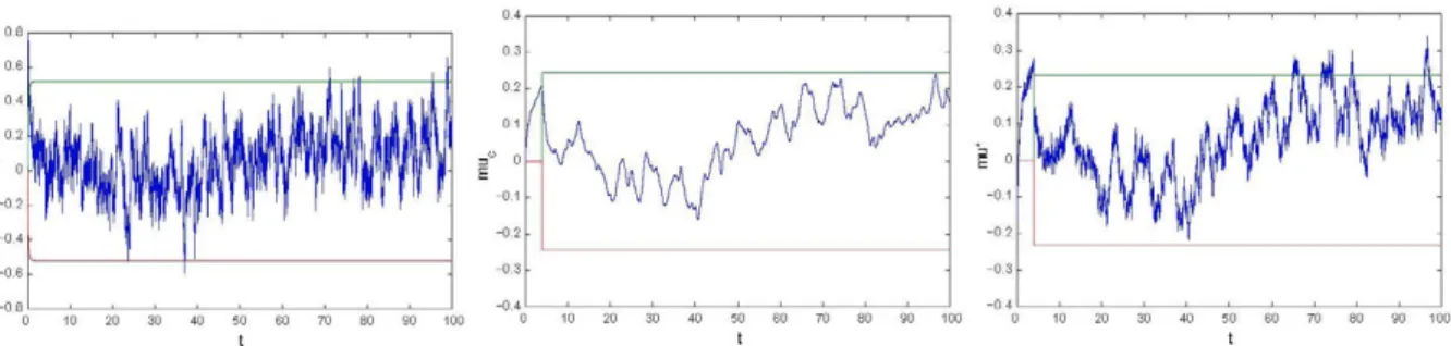
Fig. 2. Time evolution of detection schemes based on fia(t), fic(t) and fi'(t), for T = 4 and 1 = 2.

We consider that the detection schemes can measure the system state space variables; hence, defining: x(t) = -A(x(t)-x(t)) +/(x(t)), x(0) = x(0); f(x) = [fi(X1,X2),/2(X1,X2)]r

the residual e(t) = x(t) - x(t) follows the stochastic differential equation: e(t) = -Ae(t) + t](t) + s(t - Tom), e(0) = 0,

whose solution takes the form of (2). The conditional expectations are:

A = - 5 I2

mt)/Ho]

mtyHi

_{03 f}

0

e~

f-^dx

since the first residual component has zero mean before and after the fault, only the second component will be employed. We apply the sliding window scheme proposed in (12) with ¡t of (8) as a sufficient estimator measure. Different values of the window size l a n d the drift parameter 1 are considered in order to compare this scheme (based on ¡t) with the detection schemes proposed in [13,14] (based on estimators ¡ia and ¡ic). The selected test sizes have been y-, = y2 = 0.001 providing the

tests acceptance regions (—3.29^/Varil/H0(t), 3.29^/Varil/H0(t)], for the corresponding fi e \}ia,iic, (i*\ (stationary variance val-ues have been considered). When any of the estimators crosses the frontier of its corresponding acceptance region an alarm is triggered, indicating that it is likely a fault has occurred in the system.

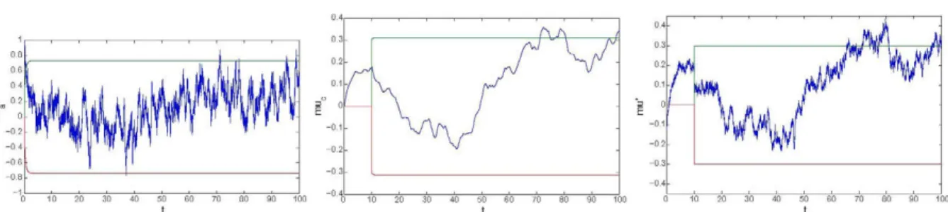
Fig. 1 shows a sample realization of mean estimators /xa(t), /xc(t) and /x*(t) (as well as their corresponding bounds) for a

window size 1 = 10 and drift 1 = 1. Note that the computations for /xc(t) and /x*(t) have only meaning for t > T. Scheme ¡ia is the only one presenting false alarm (at (Jad)H = 37,08) before the occurrence of the fault. After T0, the schemes trigger the

alarm at Tad = 70,99, Tcd = 71,23, and T*d = 65,46 respectively. Clearly, ¡t outperforms the other detection schemes: it

com-bines the fast dynamics of /xa(t) and the filtered tendency of /xc(t), to provide an good trade-of between robustness against

false alarms and sensitivity to faults. This behavior is typical in a wide range of values of 1 e [1,10]. For smaller values of 1, the scheme ¡t may trigger some false alarms (its behavior approaching that of ¡ia)\ for very large values of X, the scheme ¡t

approaches the conservative behavior of fic, but it is a bit more sensitive to faults.

Fig. 2 shows a sample realization of mean estimators /xa(t), /xc(t) and /x*(t) (as well as their corresponding bounds) for a

window size 1 = 4 and drift 1 = 2. Scheme fia is the only one presenting several false alarms (the first one at (Jd)H = 2 1 , 2 )

before the occurrence of the fault. After T0, the schemes fia and ¡t trigger the alarm at Tad = 71.01, and T*d = 64,97, whereas fic does not even fire the alarm in the considered range of time. Again, ¡t outperforms the other detection schemes. This behavior for T = 4 is typical in a wide range of values of 1 e [1,10] (in cases where fic detects the fault it does so with Tcd > 90). Note that with this smaller value of I, the scheme ¡i* provides an excellent trade-of between robustness and

sensitivity.

7. Concluding remarks

A unified setting has been defined for quickest detection of changes in continuous-time residual stochastic processes. Log-likelihood ratios have been provided for the Ornstein-Uhlenbeck process under different fault situations. A CUSUM-type approximation algorithm has also been proposed which makes use of the log-likelihood functions into a simplifying sliding window scheme. The unified setting, successfully gathers, depending on different types of simplifications, the existing detec-tion schemes for continuous-time stochastic dynamical systems [12-14,41-43,50]. This general formuladetec-tion allows for the definition of new detection schemes and for a comparative analysis among them. A simulation example has illustrated also these facts.

Acknowledgement

This work has been partially supported by project MTM2007-62064 of the Plan Nacional de I+D+i, MEyC, Spain, project MTM2010-15102 of Ministerio de Ciencia e Innovación, Spain, and by projects Q09 0930-182 and Q.10 0930-144 of the Uni-versidad Politécnica de Madrid (UPM), Spain.

Appendix A. Proof of Theorem 4.1

Given the deterministic vector function e<¡,(t), the Gaussian distribution of e(t) is totally determined by the distribution of e,(t) = [e,1(t),...,e,n(t)]. Hence, we only need to compute R(U,t2) =£[e,(t1)ej(t2)]:

R{tut2)=E e-A^-^r]{xl)dxl / rf {x2)e-A^-z^ dx2

o Jo

min(t,,t2)

0 Jo

m-i)£e-A(t2-t: _{dx = -}-m-h\ _e-m+h) 2X

e-A^-^E[r]{xl)r]T{x2)\e-A^-'í^dxldx2

e-m-h\ 21

since A = 1I„. Let us now consider a sample of vector e = [e(ti),..., e(tN)], with 0 = U <t2 < ... <tN = t, which can be reor-dered as the vector of N n components e = [ei(ti),... ,ei(tN),e2(ti),... , e2(tN),... ,e„(ti),... ,en(tN)]. Then

1 /o(e)

( 2 ^ ^ q

_e-l?C-'e

with

C = CN (g) E, and CN 2).

e-Ah-k\ \ e-i\h-h\

e-i\t-h i ₁

2 l '

1

e-„-(N-l)lM ₁

where <g> stands for the Kronecker product of matrices [32], and uniform sampling ti+i - t, = St has been considered in the last equality. The inverse takes the form

r1 = CN 1® Z -1, with CN :=

-0

0

0

1 (e'M + e-'M) - 1

- 1 eiát

Considering a similar sampling procedure for the known vector sequence e<¡,(t), the log-likelihood ratio versus the zero-mean hypothesis (e<¡,(t) = 0) becomes

_! 2/1

N g i á t _ g-XSt

rem - 1 0 0 0 (e'M - 1 + e-- 1 -iát\ 0 - 1 (eiát +

e-0 0

- i á t \

0 0 - 1

- 1 0

LR(e) = In Ti(g)'

/o(e). = ln - e L <=</•-J6* e* ~~ v£- 2e* i L e* - gist _iát _ p-lM e

N - l

(e(0) - l

, ( 0 ) )

£ - V % ( 0 ) - e,(r

)) + (e(t) - £,(t))

£-V%(r) - e ^ r ^ ) ) + ¿(e(t

)

Z 1=2

1

2 e , ( t() ),2 rI( ( e - "t + e " % ( t() - e ^ ) - e,(t(+1))

We now consider the limit when N —> oo for a fixed interval [0, t] (i.e., St = j¡ —> 0). The limit of the first terms is straight-forward and the remaining sum can be written as

2 A ¿ ( e ( t , ) - i e * ( t ( )>) Z-'fituSQSt and it can be proved that

lim f(ti,5t):

(t,«H(ti,0)

r e ^ f i ) - e^(t,-)

by using polar (r, 0) incremental coordinates around (t¡, 0) and applying L'Hopital's rule to the r —> 0 limit. Hence, f(t¡, St) can be continuously defined in a compact set [0, t] x [-a,a], a > 0, which concludes its uniform continuity. Therefore,/(t¡,¿t) converges to g"(t¡) when ¿t —> 0 uniformly in [0, t]. We can then define:

M* = max||f(t(,át)-g(t()||, such that limjt-oJWa = 0.

Hence, coming back to the sum:

S(St) = 2 ^ ( e ( t ¡ ) —em) Z-1g(t,)St + 2Xj2(e(tt) - ^ ( t , - ) ) ^ V f t , » ) -g(t,))St = S^át) + S2(«). Since e(t) is a finite covariance MS-continuous process, the first term converges in Mean Square sense to:

5l(áí)

*-ojf (

£(T)

-W

T)

) ^tf^W ~ ^

T

))

dT

'

whereas the second term can be bounded by:

N - l / 1 \ T

\S2{5t)\ = 2X ¿2(e{t() -\e,(t^VVaKtf) " / f t ) ) » < 2 l ] T ( e ( t() - l e , ( t() ) Z-1 ||/í t(t()-g(t())||át

2AMát]T ^ ( t() - Í e * ( t() ) ^ áí = 2AMMS3(áí). Taking the limit on the bound:

\S2(St)\^2XM3tS3(St)st-£0,

because lima_0S3(¿t) is a bounded integral due to the finite covariance and MS-continuity of e(t). Therefore S2(S) —r 0 implying that S(St) has the same MS-integral limit as Si (ó), and we conclude (4).

Appendix B. Proof of Corollary 4.3

Making e<¡, = ¡i in (4) we obtain:

LR£(0,t)= (e(0)-^fi\ Z-H[i+(e{t)-^i?J Z^Xfi- X2 / ( e ( T ) - - / i ) S^fidt

= x(e(Q) + e(t) + X j e(x)dx) Z~V - f l + y V ^ >

/•f iT r /•'

e(0) + e(t) + 1 / e(T)dt S'1 e(0) + e(t) + A / e(T)dt

JO J L Jo .

Taking the maximum:

CLRe(Q, t) = maxLRe(Q, t) =

where

2(2 + Xt)

H* = e{Q) + e{t) + xf0e{x)dx 2 + Xt

is the maximum likelihood estimator of ¡i. Appendix C. Proof of Lemma 4.1

Defining the generalized log-likelihood ratio:

CLR(e) = In max _{<* /o(e(ti),...,e(t}/ i ( e ( t i ) , . . . , e(tN))'

N)). which after some calculations:

In

- ! ( £ - £ * ) ' C-'(£-£*

max-e_2

CLR{e)

Mt _ p-)M

eÁdt — e i(U)E-\eme(U) - e(t

2)) + e^lT1 {e'Me(tN) - e(tN^)) + ^ ( t , - ) ^1 ( (e^ + e'MMU)

-e(tf-i) -e(ti+i))

Taking the limit when N —> oo for a fixed interval (or, equivalently, making St = ^ —> 0) we can formally proceed as in the proof of Appendix A; we can then formally integrate the result by parts to obtain (9). Note that such stochastic integral involving the squared derivative of e(t) will not exist in the usual MS, Stratonovich or Ito sense.

Appendix D. Proof of Lemma 4.2

Note that the joint distribution of [e/(t¡), and C71 are known. Let us note that:

, e/(ti)] whose covariance matrix C, is the same as for [e,-(ti),..., e/(t¡)] where C,

Ci 1

2A

I e- A | i i - t2| e- A | t i - t3| e—A|i2—ill I e-A|t2-t3|

e- A | t - i i |

= 1

Ci,i-1

Ut , i - 1

C i - i

^ L _ L ! [i;e-J.(ti .-t,- 2);e-J.(ti ,-t,- 3);. . . ;e-»(ti ,-t,)]_ I f w e m a k e t. _ ,,_., = stj j = 2 >

"I* e % 'i l) ["-j p-kSt p-2>M p-(i-2)XSt]

,¿ — 1, this expression sim-so that Cy_, = <

plifies to 'Cy_, =" "2i; " [l,e~A°l,e~ZA°l,...,e~

Considering all the components of e(t), we define the vector e = [£](£:,•),e2(t¡), • ••,en(t¡),ei(t¡-i), • •• ,en(ti)]. whose covari-ance matrix is given by:

£<g>C

=

s

. £ ® C¿,¿-i

siacs./

S ® C ¿ _ i

It is a known result [24] that:

€((,_!) - E f t t ^ ) ] E[e(t()/e(t(_i), • • •,e(ti)] = E[e(t()] + ( z ® Cj,^) f^1 ® Q\)

e(ti)-E[e(tt)]

Hence, if we consider E[e(t,)/H0] = 0 , Vj = 1 , . . . , i, and after some calculations the expression simplifies to:

e-m-t¡-i)

EH0[e(t,)/e(tf-i),..., e(ti)]

_(^

which confirms the Markov property of e(t). Hence, for the continuous time version, if we take the limit when i - 1 ) for a fixed interval (or, equivalently, making St = - 0):

limEHo[e(t¡)/e(t¡-i), we directly obtain (10). References

, e{U)} = EHo [e(t,)/e(T), 0 < T < t,^] = e ^ ' - ^ >€((,_!),

[1] E. Alcorta-Garcia, P.M. Frank, Deterministic nonlinear observer-based approaches to fault diagnosis: a survey, IFAC Control Engineering Practice 5 (1997) 663-670.

[2] M. Arató, Linear Stochastic Systems with Constant Coefficients LNCIS, vol. 45, Springer Verlag, 1982.

[3] M. Arató, S. Fegyverneki, New statistical investigations on the Ornstein-Uhlenbeck process, Computers and Mathematics with Applications 44 (2002) 677-692.

[4] S. Baran, G. Gap, M.C.A. van Zuijlen, Estimation of the mean of stationary and nonstationary Ornstein-Uhlenbeck processes and sheets, Computers and Mathematics with Applications 45 (2003) 563-579.

[5] M. Basseville, I.V. Nikiforov, Detection of Abrupt Changes, Theory and Application, Prentice Hall, 1993.

[6] G. Baxter, A strong limit theorem for Gaussian processes, Proceedings of the American Mathematical Society 7 (1956) 522-525. ¡7] M. Beibel, A note on Ritov's Bayes approach to the minimax property of the CUSUM procedure, Annals of Statistics 24 (1996) 1804-1812. ¡8] A. Berlinet, C. Thomas-Agnan, Reproducing Kernel Hilbert Spaces in Probability and Statistics, Kluwer Academic Publishers, 2004. [9] P. Billingsley, Probability and Measure, John Wiley & Sons, 1995.

[10] J.P.N. Bishwal, A. Bose, Rates of convergence of approximate maximum-likelihood estimators in the Orstein-Uhlenbeck process, Computers and Mathematics with Applications 42 (2001) 23-38.

[11] I.F. Blake, W.C. Lindsey, Level-crossing problem for random processes, IEEE Transactions on Information Theory 19 (35) (1973) 295-315. May. [12] Á. Castillo, P. Zufiria, M.M. Polycarpou, F. Previdi, T. Parisini, Fault detection and isolation scheme in continuous time nonlinear stochastic systems, in:

Proceedings of the 5th IFAC Symposium on Fault Detection, Supervision and Safety of Technical Processes SAFEPROCESS 2003, 2003, pp. 651-656. [13] Á. Castillo, Fault Detection and Isolation via Continuous Time Statistics, Ph.D. thesis, E.T.S. Ingenieros Industriales (Universidad Politécnica de Madrid),

[14] A. Castillo, P. Zufiria, Fault detection schemes for continuous-time stochastic dynamical systems, IEEE Transactions on Automatic Control 54 (8) (2009) 1820-1836.

[15] J. Chen, R. Patton, Robust Model-Based Fault Diagnosis for Dynamic Systems, Kluwer Academic Publishers, 1999.

[16] E. Csáki, D. Khoshnevisan, Capacity estimates boundary crossings and the Ornstein-Uhlenbeck process in Wiener space, Eletronic Communications in Probability 4 (1999) 103-109.

[17] C. De Persis, A. Isidori, A geometric approach to nonlinear fault detection and isolation, IEEE Transactions on Automatic Control 46 (2001) 853-865. [18] D. Florens-Landais, H. Pham, Large deviations in estimation of an Ornstein-Uhlenbeck model, Journal of Applied Probability 36 (1999) 60-77. [19] P.M. Frank, Analytical and qualitative model-based fault diagnosis - a survey and some new results, European Journal of Control 11 (2) (1996) 26-28. [20] J.J. Gertler, Fault Detection and Diagnosis in Engineering Systems, Marcel Dekker, New York, 1998.

[21] M. Ghosh, N. Mukhopadhyay, P.K. Sen, Sequential Estimation, Wiley Series in Probability and Statistics (1997). [22] Z. Govindarajulu, Sequential Statistics, World Scientific, 2004.

[23] R. Iserman, Fault-Diagnosis Systems, An Introduction to Fault Detection and Fault Tolerance, Springer Verlag, 2006. [24] R.A Johnson, D.W. Wichern, Applied Multivariable Statistical Analysis, Prentice Hall, 1992.

[25] T. Kailath, A RKHS approach to detection and estimation problems—part I: Deterministic signals in gaussian noise, IEEE Transactions on Information Theory 17 (5) (1971) 530-549.

[26] T. Kailath, H.V. Poor, Detection of stochastic processes, IEEE Transactions on Information Theory 44 (6) (1998) 2230-2259. [27] I. Karatzas, S.E. Shreve, Brownian Motion and Stochastic Calculus, Springer Verlag, 1988.

[28] J. Klamka, Stochastic controllability of linear systems with state delays, International Journal of Applied Mathematics and Computer Science 17 (1) (2007) 5-13.

[29] J. Klamka, Stochastic controllability and minimum energy control of systems with multiple delays in control, Applied Mathematics and Computation 2 0 6 ( 2 ) ( 2 0 0 8 ) 7 0 4 - 7 1 5 .

[30] M.L. Kleptsyna, A. Le Breton, Statistical analysis of the fractional Ornstein-Uhlenbeck type process, Statistical Inference for Stochastic Processes 5 (2002) 229-248.

[31 ] T.L. Lai, Sequential multiple hypothesis testing and efficient fault detection-isolation in stochastic systems, IEEE Transactions on Information Theory 46 (2) (2000) 595-608.

[32] P. Lancaster, M. Tismenetsky, The Theory of Matrices, second ed., Academic Press, 1985.

[33] H.M. Larson, B.O. Shubert, Probabilistic Models in Engineering Sciences, vol. I, John Wiley and Sons, 1979.

[34] R.S. Liptser, A.N. Shiryaev, Statistics of Random Processes. I. General Theory, second ed., Springer Verlag, Kluwer Academic Publishers, 2001. [35] R.S. Liptser, A.N. Shiryaev, Statistics of Random Processes. II. Applications, second ed., Springer Verlag, Kluwer Academic Publishers, 2001. [36] G. Lorden, Procedures for reacting to a change in distribution, Annals of Mathematical Statistics 42 (1971) 1897-1908.

[37] D.R. Morgan, On level-crossing excursions of Gaussian low-pass random processes, IEEE Transactions on Signal Processing 55 (7) (2007) 3623-3632. [38] G.V. Moustakides, Optimal stopping times for detecting changes in distributions, Annals of Statistics 14 (1986) 1379-1387.

[39] G.V. Moustakides, Quickest detection of abrupt changes for a class of random processes, IEEE Transactions on Information Theory 44 (5) (1998) 1965-1968.

[40] G.V. Moustakides, Optimality of the CUSUM procedure in continuous time, Annals of Statistics 32 (1) (2004) 302-315.

[41] U. Münz, Parametric Fault Diagnosis in Stochastic Systems, Masters thesis, E.T.S. Ingenieros Telecomunicación (Universidad Politcnica de Madrid), 2005.

[42] U. Münz, P. Zufiria, Parametric Fault Diagnosis in Stochastic Dynamical Systems, in: Proceedings of the 19th CEDYA, Madrid, Spain, 2005. [43] U. Münz, P. Zufiria, Diagnosis of unknown parametric faults in non-linear stochastic dynamical systems, International Journal of Control 82 (4) (2009)

603-619.

[44] I.V. Nikiforov, Two strategies in the problem of change detection and isolation, IEEE Transactions on Information Theory 43 (2) (1997) 770-776. [45] E.S. Page, Continuous inspection schemes, Biometrika 41 (1/2) (1954) 100-115.

[46] M.M. Polycarpou, A.T. Vemuri, Learning Methodology for Failure Detection and Accomodation, IEEE Control Systems (1995) 16-24.

[47] M.M. Polycarpou, A.B. Trunov, Learning approach to nonlinear fault diagnosis: detectability analysis, IEEE Transactions on Automatic Control 45 (2000) 806-812.

[48] H.V. Poor, An Introduction to Signal Detection and Estimation, second ed., Springer Verlag, 1994. [49] H.V. Poor, O. Hadjiliadis, Quickest Detection, Cambridge University Press, 2009.

[50] M. Reble, U. Münz, F. Allgower, Diagnosis of parametric faults in multivariable nonlinear systems, in: Proceedings of the 46th IEEE Conference on Decision and Control Conference 2007, 2007, pp. 336-371.

[51 ] R. Riaza, P.J. Zufiria, Differentialalgebraic equations and singular perturbation methods in recurrent neural learning, Dynamical Systems 18 (2003) 8 9 -105.

[52] A. Szimayer, R. Mailer, Testing for mean reversion in processes of OrnsteinUhlenbeck type, Statistical Inference for Stochastic Processes 7 (2004) 9 5 -113.

[53] A.N. Shiryaev, On optimum methods in quickest detection problems, Theory of Probability and its Applications VIII (1) (1963) 22-46. [54] A.N. Shiryaev, Optimal Stopping Rules, Springer Verlag, 1978.

[55] A.N. Shiryaev, Minimax optimality of the method of cumulative sums (cusum) in the case of continuous time, Communications of the Moscow Mathematical Society (1996) 750-751.

[56] D. Siegmund, Sequential Analysis, Tests and Confidence Intervals, Springer Verlag, 1985. [57] H.L. Van Trees, Detection, Estimation and Modulation Theory: Part I, Wiley, 1968. [58] A. Wald, Sequential Analysis, John Wiley & Sons, 1947.

[59] A.S. Willsky, H.L Jones, A generalized likelihood ratio approach to the detection and estimation of jumps in linear systems, IEEE Transactions on Automatic Control AC-21 (1976) 108-112.