UNIVERSIDAD NACIONAL DE INGENIERÍA
FACULTAD DE CIENCIAS
TESIS
“
FORECAST MODELING OF SPATIO-TEMPORAL RASTERDATA USING PRINCIPAL COMPONENT ANALYSIS AND A
NEURAL NETWORKS – WAVELET DECOMPOSITION MODEL
”
PARA OPTAR EL GRADO ACADEMICO DE MAESTRO EN CIENCIAS EN MATEMÁTICA APLICADA
PRESENTADA POR
CHRISTIAN AMAO SUXO
Asesor
Dr. OSWALDO JOSÉ VELÁSQUEZ CASTAÑÓN Asesor externo
Dr. CARLOS ANTONIO ABANTO VALLE
ACKNOWLEDGEMENTS
I would first like to thank my external thesis advisor Ph.D. Carlos Antonio Abanto Valle of the
school of statistics at the Federal University of Rio de Janeiro. Prof. Abanto was always attentive
to my needs whenever I ran into a trouble spot or had a question about my research or writing. He
consistently allowed this thesis to be my own work, but steered me in the right direction whenever
he thought I needed it. I am forever grateful to you.
I would also like to thank the other expert proffesors who were involved in the realization of
this research project. Thanks to Ph.D. Loretta Betzabe Rosa Gasco Campos and Dr. Alipio
Fran-cisco Ord´o˜nez Mercado who gladly accepted to be my thesis reviewers. Without their passionate
participation and helpful input, the thesis would not have been successfully conducted. A special
thanks to Ph.D. Oswaldo Jose Vel´asquez Casta˜n´on and Ph.D. Eladio Te´ofilo Oca˜na Anaya,
profes-sors of the master that wholeheartedly helped me with diverse burocratic processes. Without your
support, the thesis would not have reached the sufficient formal requirements to be admitted.
Finally, I must express my very profound gratitude to my family and my unconditional friends
for providing me with unfailing support and continuous encouragement throughout my master’s
studies and through the process of researching and writing this thesis. This accomplishment would
ABSTRACT
Forecast modeling of spatio-temporal raster data using
principal component analysis and a neural networks - wavelet
decomposition model
Christian Amao Suxo
Advisor: Oswaldo Jos´
e Vel´
asquez Casta˜
n´
on
Nowadays spatio-temporal forecasting has been drawing more and more attention from
aca-demic researchers and industrial practitioners for its great utility to plan and develop contingency
measures against future adverse conditions. In this thesis, a methodology to forecast maps in
spatio-temporal raster datasets is proposed. Following a summarize-predict-and-rebuild methodology, it
1) first suggests a reduction in the dimensionality of data using a principal component analysis,
then 2) individual forecasts on the most significant components or eigenvectors are calculated using
a neural networks - wavelet decomposition model. Finally, 3) a recursive algorithm, applied on the
spectral inverse reconstruction of the individual forecasts, provides the final forecast maps.
The devised methodology led to three models according: the spatial principal component
anal-ysis (SPCA) model, the temporal principal component analanal-ysis (TPCA) model and the
spatio-temporal principal component analysis (STPCA) model. In order to evaluate their forecasting
accuracy, a simulation study was carried out by considering datasets with pure temporal, pure
spatial and spatio-temporal variability. The results suggest using a TPCA (or SPCA) model when
the temporal (or spatial) variability is predominant. For datasets with similar spatial and temporal
variability information, the STPCA model provides the best forecast results. The research
culmi-nates with a real-world case study in monthly sea surface temperature anomalies of the Tropical
Pacific Ocean.
RESUMEN
Modelado de pron´
ostico en datos espacio-temporales tipo
raster usando un an´
alisis de componentes principales y un
modelo de redes neuronales con descomposici´
on de ond´ıculas
Autor: Christian Amao Suxo
Asesor: Oswaldo Jos´
e Vel´
asquez Casta˜
n´
on
En la actualidad, el pron´ostico de datos espacio-temporales ha sido de especial inter´es para
investigadores acad´emicos y profesionales de la industria por su gran utilidad para planificar y
desarrollar medidas de contingencia contra futuras condiciones adversas. En este trabajo se
pro-pone una metodolog´ıa para el pron´ostico de mapas tipo raster. Siguiendo una metodolog´ıa de
resumir-predecir-y-reconstruir, el m´etodo sugiere reducir la dimensionalidad de los datos usando
un an´alisis de componentes principales para luego realizar pron´osticos individuales sobre las
com-ponentes o autovectores m´as significativos. Finalmente, un algoritmo recursivo, aplicado sobre la
reconstrucci´on inversa espectral de los pron´osticos individuales, brinda el pron´osticos final de los
mapas.
La metodolog´ıa propuesta da lugar a tres modelos: el modelo espacial de componentes
princi-pales (ECP), el modelo temporal de componentes principrinci-pales (TCP) y el modelo espacio-temporal
de componentes principales (ETCP). Con el fin de evaluar su capacidad de pron´ostico, se
real-iza un estudio de simulaci´on considerando datos con una estructura de variabilidad espacial pura,
temporal pura y espacio-temporal. Los resultados sugieren usar un modelo TCP (o ECP) cuando
la variabilidad temporal (o espacial) es predominante. Para datos con similar informaci´on en la
variabilidad espacial y temporal, el modelo ETCP brinda los mejores resultados de pron´ostico. El
trabajo culmina con una aplicaci´on real en datos mensuales de anomal´ıas de temperatura superficial
del mar del oc´eano Pac´ıfico Tropical.
Contents
1 Introduction 12
2 Preliminaries 15
2.1 Introduction. . . 15
2.2 Raster datasets . . . 15
2.3 Qualitative analysis of spatio-temporal raster datasets . . . 17
2.3.1 Analysis of time series: the temporal variability. . . 19
2.3.2 Analysis of spatial datasets: the spatial variability . . . 21
2.3.3 Analysis of spatio-temporal datasets: the spatio-temporal variability . . . 25
2.4 Principal Component Analysis . . . 27
2.4.1 Population principal components . . . 28
2.4.2 Sample principal components . . . 32
2.4.3 PCA in a spatio-temporal context . . . 34
2.4.4 How many principal components to retain? . . . 37
2.5 Autoregressive Neural Network model . . . 40
2.5.1 Artificial Neural Networks . . . 40
2.5.2 Autoregressive processes . . . 42
2.5.3 The AR-NN structure . . . 43
2.5.4 Modelling univariate AR-NN processes . . . 46
2.6 Wavelet decomposition of discrete time series . . . 53
2.6.2 Multiresolution Analysis . . . 56
2.6.3 Discrete Wavelet Transform (DWT) . . . 59
2.6.4 Pyramid Algorithm: the filtering approach . . . 65
2.6.5 Maximal Overlap Discrete Wavelet Transform (MODWT) . . . 69
3 Proposed methods for spatio-temporal modeling of raster datasets 72 3.1 Introduction. . . 72
3.2 The Temporal Principal Component Analysis model . . . 73
3.3 The Spatial Principal Component Analysis model . . . 77
3.4 The Spatio - Temporal Principal Component Analysis model . . . 81
4 Simulation study 86 4.1 The pure spatial variability process . . . 86
4.2 The pure temporal variability process . . . 88
4.3 The spatio - temporal variability process . . . 89
4.4 Simulation results . . . 90
4.5 Final comments . . . 98
5 Empirical application 104 5.1 Description of the sea surface temperature dataset . . . 106
5.2 Principal results of the application . . . 107
6 Conclusions and future developments 111 6.1 Future research directions . . . 112
List of Figures
2.1 Representation of a scanned map with a raster dataset. . . 16
2.2 An example of how are built the cell values in raster data. . . 17
2.3 An example of how a simple polygon feature is read through raster dataset at different resolutions. . . 18
2.4 Visual representation of spatio-temporal raster datasets. X and Y axes represent the coordinate system for the spatial location and theZ axis represents the temporal evolution of rasters. . . 18
2.5 A time series with the four traditional variations: trend, seasonal variations, cycle and irregular fluctuations. . . 20
2.6 Measures of earthquake magnitudes (in Richter scale) at different point locations in a bay area since 1962 to 1981. This is an example of spatial data measured in specific point locations in a continuous space. . . 22
2.7 Measurements of an atributte in the different states of the United States. This is an example of aerial data irregularly spaced. . . 23
2.8 An example of how principal component analysis works. . . 28
2.9 Scheme of how the data matrix is obtained when working with a spatio-temporal raster dataset.. . . 36
2.10 Artificial Neuron Model. . . 41
2.11 Different types of activation functions. . . 42
2.12 Architecture of an AR-NN model with one hidden layer. . . 44
2.14 Flow chart of the Levenberg-Marquardt algorithm. . . 54
2.15 DWT process following a pyramid algorithm of a discrete time series z with three levels of decomposition. The maximum frequency of z isp. . . 66
3.1 Operating scheme of the MODWT-AR-NN model. . . 75
3.2 An sketch of how to use the training period to calculate the “importance” weights.
n, Landh represent the lengths of total period, training period and forecast horizon respectively. . . 82
4.1 Spatial distribution of averaged maps of one replication in scenario: (a) PSV - Ex-ponential, (b) PSV - Mat´ern, (c) PSV - Spherical, (d) PTV - ρ = 0.5, (e) PTV
-ρ = 0.75, (f) PTV -ρ = 0.95, (g) STV Exponential, (h) STV Mat´ern, (i) STV -Spherical. The standard deviation is contoured in black. . . 91
4.2 An sketch of how to calculate the evolution of the global median of the spatial MAPE with a forecast horizon of length six. . . 93
4.3 Evolution of the global median of the spatial MAPE using the SPCA, TPCA and STPCA model in the simulated processes: (a) PSV-Exponential, (b) PSV-Mat´ern, (c) PSV-Spherical, (d) PTV-ρ = 0,5, (e) PTV-ρ = 0,75, (f) PTV-ρ = 0,95, (g) STV-Exponential, (h) STV-Mat´ern, (i) STV-Spherical. . . 94
4.4 Spatial distribution of the median MAPE (of the 50 replications) corresponding to the six forecasted periods of the PSV- Spherical process using the SPCA model. . . 95
4.5 Spatial distribution of the median MAPE (of the 50 replications) corresponding to the six forecasted periods of the PSV- Spherical process using the TPCA model. . . 96
4.6 Spatial distribution of the median MAPE (of the 50 replications) corresponding to the six forecasted periods of the PTV -ρ= 0.5 process using the SPCA model. . . . 97
4.7 Spatial distribution of the median MAPE (of the 50 replications) corresponding to the six forecasted periods of the PTV -ρ= 0.5 process using the TPCA model. . . . 98
4.9 Spatial distribution of the median MAPE (of the 50 replications) corresponding to the six forecasted periods of the STV - Mat´ern process using the TPCA model. . . . 100
4.10 Spatial distribution of the median MAPE (of the 50 replications) corresponding to the six forecasted periods of the STV - Mat´ern process using the STPCA model. . . 101
5.1 Map of the Pacific Ocean indicating, with red lines, the location of the Tropical Pacific Ocean. . . 104
5.2 Spatial distribution of the averagedSST (in◦C) of the Tropical Pacific Ocean. The value of the standard deviation of SST is contourned in black. . . 105
5.3 Evolution of the median of the spatial MAE using the TPCA, the SPCA and STPCA model over the SSTA dataset. . . 107
5.4 Spatial distribution of the median MAE when the SPCA model is used over the SSTA dataset.. . . 108
5.5 Spatial distribution of the median MAE when the TPCA model is used over the SSTA dataset.. . . 109
5.6 Spatial distribution of the median MAE when the STPCA model is used over the SSTA dataset.. . . 110
A.1 Spatial distribution of the median MAPE (of the 50 replications) corresponding to the six forecasted periods of the PSV-Exponential process using the SPCA model. . 120
A.2 Spatial distribution of the averaged MAPE (of the 50 replications) corresponding to the six forecasted periods of the PSV-Exponential process using the TPCA model. . 121
A.3 Spatial distribution of the median MAPE (of the 50 replications) corresponding to the six forecasted periods of the PSV-Exponential process using the STPCA model. 122
A.4 Spatial distribution of the averaged MAPE (of the 50 replications) corresponding to the six forecasted periods of the PSV-Mat´ern process using the SPCA model. . . 123
A.5 Spatial distribution of the median MAPE (of the 50 replications) corresponding to the six forecasted periods of the PSV-Mat´ern process using the TPCA model. . . 124
A.7 Spatial distribution of the median MAPE (of the 50 replications) corresponding to the six forecasted periods of the PSV- Spherical process using the STPCA model.. . 126
A.8 Spatial distribution of the median MAPE (of the 50 replications) corresponding to the six forecasted periods of the PTV -ρ= 0.50 process using the STPCA model. . 127
A.9 Spatial distribution of the median MAPE (of the 50 replications) corresponding to the six forecasted periods of the PTV -ρ= 0.75 process using the SPCA model. . . 128
A.10 Spatial distribution of the median MAPE (of the 50 replications) corresponding to the six forecasted periods of the PTV -ρ= 0.75 process using the TPCA model. . . 129
A.11 Spatial distribution of the median MAPE (of the 50 replications) corresponding to the six forecasted periods of the PTV -ρ= 0.75 process using the STPCA model. . 130
A.12 Spatial distribution of the median MAPE (of the 50 replications) corresponding to the six forecasted periods of the PTV -ρ= 0.95 process using the SPCA model. . . 131
A.13 Spatial distribution of the median MAPE (of the 50 replications) corresponding to the six forecasted periods of the PTV -ρ= 0.95 process using the TPCA model. . . 132
A.14 Spatial distribution of the median MAPE (of the 50 replications) corresponding to the six forecasted periods of the PTV -ρ= 0.95 process using the STPCA model. . 133
A.15 Spatial distribution of the median MAPE (of the 50 replications) corresponding to the six forecasted periods of the STV - Exponential process using the SPCA model. 134
A.16 Spatial distribution of the median MAPE (of the 50 replications) corresponding to the six forecasted periods of the STV - Exponential process using the TPCA model. 135
A.17 Spatial distribution of the median MAPE (of the 50 replications) corresponding to the six forecasted periods of the STV - Exponential process using the STPCA model.136
A.18 Spatial distribution of the median MAPE (of the 50 replications) corresponding to the six forecasted periods of the STV - Spherical process using the SPCA model. . . 137
A.19 Spatial distribution of the median MAPE (of the 50 replications) corresponding to the six forecasted periods of the STV - Spherical process using the TPCA model. . . 138
List of Tables
2.1 The six mode of decomposition and how is related to the structure of its respective data matrix X (equation (2.27)). . . 35
4.1 Table with the nine simulated processes used in the simulation study. . . 90
4.2 Global median MAPE in-sample of the nine simulated processes using the SPCA, TPCA and STPCA model. . . 92
4.3 Median of theM AP Es in the nine simulated processes using the SPCA, TPCA and STPCA model. . . 102
4.4 Median“importance” weights of the SPCA and TPCA model in the nine simulated processes. . . 103
Chapter 1
Introduction
Spatio-temporal forecasting models for raster datasets have gained widespread popularity in recent
years due to its great applicability in different fields such as agriculture, economics and
oceanog-raphy (Cressie and Majure,1997;Pace et al.,1998). Indeed, spatio-temporal forecasting has been developing from individual spatial or temporal forecasting and gained vast attention recently for
its promising performance in handling complex data, in which not only spatial but also temporal
characteristic must be taken into account. This juxtaposition of space and time into the data has
made the spatio-temporal forecasting a challenging task that requires models to take into account
the interaction of these complex dinamycs. Furthermore, spatio-temporal datasets are often large
and therefore require substantial computing resources to fit even simple models.
A brief review in literature shows that models for spatio-temporal data are usually built by
in-tegrating time series models with variogram-based models from spatial statistics. In the time series
context, popular approaches include ARMA models (Box and Jenkins,1976) for stationary data, and state-space models (Migon et al., 2005), which permit to model nonstationary components such as temporal trends and seasonality. In the spatial field, much of the literature goes around
isotropic models (Cressie and Wikle, 2015) for spatial stationary datasets. Various methods also exist for nonstationary spatial processes, where the correlation depends on location as well as
The first spatio-temporal models often relied on the assumption of temporal stationarity. For
example, the STARMA (Pfeifer and Jay Deutsch, 1980) and STARMAX (Stoffer, 1986) models were built by adding a spatial covariance structure to standard vector ARMA models. Later
models proposed methods to deal with nonstationarity and spatial anisotropy. An example of this
is the work of Guttorp et al. (1994), where with the use of the deformation technique of Sampson and Guttorp (1992) they could capture spatial anisotropy in a series of ozone readings. Wikle et al. (1998) used a hierarchical bayesian model with CAR priors for spatial effects for modeling monthly maximum atmospheric temperatures. Other approaches involving hierarchical bayesian
models using CAR priors are also found inCressie and Wikle (2015).
The main contribution of this thesis is a flexible, efficient and simple-to-manage methodology
for spatio-temporal forecasting. Following this path, this work has as main objective to evaluate the
forecast performance of a proposedsummarize-predict-and-rebuild methodology. This methodology
suggest, as first step, to reduce the dimensionality of data using a principal component analysis.
This summary of information allows to work with the essential spatio-temporal variability. At
a second step, individual forecasts on the most significant components or eigenvectors are found
using a neural networks - wavelet decomposition model. This prediction part of the methodology
allows to model only the significant information of a complex spatio-temporal dataset. Finally, the
last step consists of applying a recoursive algorithm, on the spectral inverse reconstruction of the
individual forecasts of the previous step, to provide the resulting forecast maps.
As a result of thesummarize-predict-and-rebuild methodology, three models are induced: the
temporal principal component analysis (TPCA) model, the spatial principal component analysis
(SPCA) model and the spatio-temporal principal component analysis (STPCA) model. The TPCA
and SPCA model differ in the second step of the devised methodology. While the TPCA model
applies the forecasting model on the significant principal components, the SPCA model applies the
model on the significant eigenvectors. For its side, the STPCA model behaves as an hybrid of the
TPCA and SPCA models. In fact, it integrates the good forecasting results of both models in order
to get an enhanced forecast accuracy.
The main advantage of the devised methodology is that it provides forecast maps without the
simple to deal with. The proposed model works under the philosophy of understanding the whole
knowing its parts. Indeed, the method works with the most relevant spatio-temporal variability of
the raster dataset and seeks to model, in a detailed way, the different variability components in
order to obtain an improved forecast.
This thesis is organized as follows. In chapter2, a brief summary of the principal concepts and statistical techniques used in this work are explained. Concepts such as raster datasets, stationarity,
spatial auto-covariance function, isotropy, and others are developed. Likewise, statistical methods
such as the principal component analysis, the autoregressive neural network model and the discrete
wavelet transform are also presented here. Chapter 3 displays the devised methodology of this thesis. An explicit mathematical and algorithmic description of the three proposed models are
carried out here. Chapter 4 shows the results of a simulation study for checking the prediction and forecast performance of the proposed models. Chapter 5 develops a real-world case study in monthly sea surface temperature anomalies of the Tropical Pacific Ocean with the purpose to check
Chapter 2
Preliminaries
2.1
Introduction
This chapter introduces some concepts and statistical techniques which will be used in the
de-velopment of this thesis. Section 2.2 gives a description of raster datasets. Section 2.3 describes meaningful concepts to manage spatio-temporal raster datasets. Next, section 2.4 provides the mathematical development of the principal component analysis (PCA) technique and shows a
brief literature review considering the use of the PCA to analyze spatio-temporal raster datasets.
Thereby, section 2.5 introduces autoregressive neural network (AR-NN) models and section 2.6
deals with topics related to wavelet decomposition methods and their properties.
2.2
Raster datasets
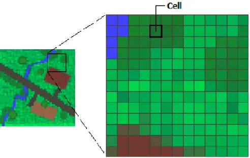
In general, a raster dataset, or simply called raster, consists of a matrix of cells (or pixels) organized
into rows and columns (or a grid) where each cell contains a value representing information. All
cells in a raster set must be the same size, determining theresolution. The cells can be of any size,
but they should be small as possible in order to accomplish a detailed analysis. In that way, a cell
can represent a square kilometer, a square meter, or even a square centimeter. Figure2.1shows an example of how this process is done.
Figure 2.1: Representation of a scanned map with a raster dataset.
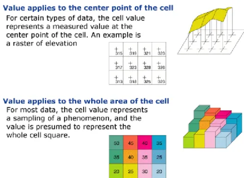
by the raster dataset such as a category, magnitude, height, or a spectral value. The category could
be a land-use class such as grassland, forest or road. A magnitude might represent gravity, noise
pollution or air temperature. Height (distance) could represent surface elevation above mean sea
level, which can be used to derive slope, aspect and watershed properties. Spectral values are used
in satellite imagery and aerial photography to represent light reflectance and color. For purposes
of this work, the cell values will represent a magnitude.
Cell values can be either positive or negative, integer, or floating point. Integer values are used
to represent categorical (discrete) data, and floating point values to represent continuous surfaces.
Cells can also have a missing value to represent the absence of data. Figure 2.2gives an idea what can represent the cell values. A cell value could represent the magnitude value in the center point
of the cell or the entire area of the cell. For experimental and empirical analysis of this thesis the
second option is considered.
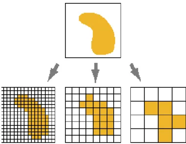
The dimension of the cells must be chosen according to the analysis necessities. In fact, the
cells can be as large or as small as needed to represent the surface conveyed by the raster dataset
and the features within the surface. The size of the cell determines how coarse or fine the patterns
Figure 2.2: An example of how are built the cell values in raster data.
raster will be. However, the greater the number of cells, the longer it will take to process all the
available information and it will increase the demand for storage space. If a cell size is too large,
information may be lost or subtle patterns may be obscured. For example, if the cell size is larger
than the width of a road, the road may not exist within the raster dataset. Figure 2.3shows how a simple polygon feature will be represented by a raster dataset at various cell sizes.
As it was described, process of raster clearly results in a loss of information, from the real-valued
coordinates of the points, through the integer cell counts. However, there are multiple gains. First
one, the data structure is more compact and easy to visualize. Furthermore, it can be related
to other rasters provided the locations and resolutions are properly conflated wherewith complex
spatial statistical analysis could be performed.
2.3
Qualitative analysis of spatio-temporal raster datasets
Spatio-temporal raster datasets are raster datasets with an intrinsic temporal component, i. e. the
Figure 2.3: An example of how a simple polygon feature is read through raster dataset at different resolutions.
region collected over a period of time is an example of this kind of data. Figure 2.4 displays how the spatial and temporal dimensions are portrayed in spatio-temporal raster datasets.
𝑿
𝒀
𝒁
𝒕
𝟏
𝒕
𝟐
𝒕
𝟑
Figure 2.4: Visual representation of spatio-temporal raster datasets. X and Y axes represent
Due to the intrinsic spatial and temporal dimensions, the spatio-temporal statistical analysis is
concerned with data variation in space and time. Hence the statistical effort will be concentrated
in the analysis of temporal variability, spatial variability and its possible interactions. In order to
deal with these problems, next subsections describe some necessary statistical concepts.
2.3.1 Analysis of time series: the temporal variability
Definition 1. For a given probability space (Ω,F,P) and a measurable space (S,S), a stochastic
process is a collection of S−valued random variables which can be written as
{X(t) :t∈P}. (2.1)
Where S andP are known as the state space and parameter space of the stochastic process. IfT is discrete (continuous), equation 2.1 is called a discrete (continuous) stochastic process.
Atime series can be seen as a realization of a stochastic process with a discrete-time observation
support. In other words, a time series is a collection of observations made sequentally in time and
indexed by integers. A time series shall be represented by the discrete stochastic process {xt}Tt=1,
whereT represents the length of the series. According to the number of variables analyzed through time, a time series can be eitherunivariate (xt∈R) or multivariate (xt∈Rn, n >1).
Two of the main goals of the analysis of time series are modeling and forecasting. The aim of
modeling is to find a mechanism to describe the data generation process. In theory, this requires
a complete knowledge of the laws of physics, biology, etc., which govern the evolution of the
environment related to the involved time series. However, in practice there is little or no prior
knowledge about all the factors that influence the evolution. In that case, it is possible to build
a model using only the information coming from the time series, by studying its behavior in the
past. In general, a good model should capture essential features of the long-term behavior of the
system. On the other hand, the goal of forecasting, or predicting, is mainly to predict the future
short-term evolution of the system. These two goals are not necessarily intersecting: a model that
properly describes long-term governing mechanisms may fail in giving reliable short-term forecasts;
give) a good insight into the long-term properties of the system (Qi and Zhang,2001). The present thesis has as main objective the forecast.
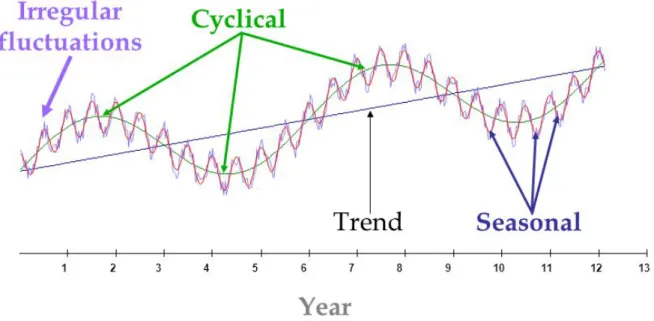
Traditionally, methods of time series analysis are mainly concerned with decomposing the total
variation of a series into four components of variability: trend, seasonal variation, cycle, and
irregular fluctuations (see figure 2.5). These variation components do not usually occur alone; in fact, they can occur in any combination or can occur all together (Qi and Zhang,2001).
Figure 2.5: A time series with the four traditional variations: trend, seasonal variations, cycle
and irregular fluctuations.
The crucial difference between time series, and situations usually considered in classical
statis-tics, is that the measurementsxm andxn;m6=n, will be stochastically dependent. Indeed, almost
always a sequence of measurements made in equally spaced time instants is regarded as a
realiza-tion of a process which, in principle, has continuous sample paths {xt}t∈R. Then, as s and t get
close, the variables xs and xt tend to be dependent. However, the way how they depend defines
the stationarity of the time series.
Definition 2. A time series {xt}∞t=1 is weak stationary (or simply called stationary) if:
2. V(xt) =σ2 for all t,
3. γ(xt1, xt2) =f(t2−t1) for t1< t2,
where V(.) and γ(., .) denote the variance and the auto-covariance function, respectively.
Condition 1 definesfirst-order stationarityand conditions 2 and 3 definesecond-order
stationar-ity. Both concepts give place to the stationarity. This concept is important since most forecasting
methods assume that involved time series are stationary. An absence of stationarity can cause
un-expected or bizarre behaviors, like t-ratios not following a t-distribution or high R-squared values assigned to variables that are not correlated at all. However, in real applications time series are
not stationaries but data can be stationarized through mathematical transformations.
Statistical performance measures
In this study, several measures to evaluate the performance of different forecasting models are
employed. Given a time series {xt}Tt=1 and corresponding predicted values ˆxt, the performance
measures to evaluate in-sample (adjustment) and out-sample (forecast) results are defined as
1. The Mean Absolute Error (MAE)
M AE = 1
T
T
X
t=1
|xt−xˆt|. (2.2)
2. Mean Absolute Percentage Error (MAPE)
M AP E= 1
T
T
X
t=1
|xt−xˆt| |xt| ×
100%. (2.3)
2.3.2 Analysis of spatial datasets: the spatial variability
Spatial data are geo-referenced attribute measurements (continuous or discrete) where each
mea-surement is associated with a location (point) or an entity (region or object) in a geographical
on a regular lattice (rasters) or scattered in space (see figure 2.6). The domain informed by a measurement is called the sample unit, e.g. pixels (or cells) for raster datasets.
C. Funk Geog 210C Spring 2010
1
9
Point Pattern Data
Characteristics
Series of point locations with recorded “events", e.g., locations of
trees, disease or crime incidents
Point locations correspond to all possible events (mapped point
pattern), or to a subset (sampled point pattern)
Attribute values also possible at same locations, e.g., tree
diameter, magnitude of earthquakes (marked point pattern)
Figure 2.6: Measures of earthquake magnitudes (in Richter scale) at different point locations in a
bay area since 1962 to 1981. This is an example of spatial data measured in specific point locations in a continuous space.
Formally, spatial statistics deals with the analysis of realizations of a stochastic process
{Zs:s∈D⊂Rp, p >0}; (2.4)
where s is the location in the p-dimensional Euclidean space and Zs is a random variable in the
locations. In this thesis, the interest is concentrated when p= 2.
According to the nature ofD in equation (2.4), spatial statistics is subdivided into three large fields:
1. Geostatistics: It studies data of stochastic processes in which the parameter space D⊂R2 is
continuous. However, in practice it depends on the researcher to select in which sites of the
region of interest the measurement of the variables is made, that is, the researcher can select
it is said that the setDis fixed. It is important to highlight that in geostatistics the essential purpose is interpolation due to the spatial continuity.
2. Aerial data analysis: In this case the involved stochastic process has a discrete parameter
space D ⊂R2 and the selection of the measurement sites depends on the researcher, i.e. D
is fixed. The sampling locations may be regularly (such as rasters) or irregularly spaced (see
figure 2.7). The essential purpose of the analysis is to detect and model spatial patterns or trends in area values. Spatial interpolation is meaningless in this context unless it is necessary
to input missing values.
Figure 2.7: Measurements of an atributte in the different states of the United States. This is an
example of aerial data irregularly spaced.
3. Point patterns: The main difference of the point pattern analysis with the two fields mentioned
above lies in the fact thatD⊂R2 is not fixed. D can be discrete or continuous but the site
locations where the phenomenon to be studied occurs is given by nature. In general, here the
main purpose is to determine if the distribution of individuals within the region is random,
aggregate or uniform. Figure2.6 shows an example of spatial point pattern.
A very important stage in the analysis of spatial data is the determination of the spatial
the association or similarity of the values according to the distance between them is by itself a result
that allows to characterize the population in study and is also fundamental in the development of
prediction models. So, the concept of spatial autocovariance function is introduced next.
Definition 3. Given a spatial process {Zs :s∈D⊂R2}, the spatial auto-covariance function is
defined as
C(s1, s2) =Cov(Zs1, Zs2) =E[(Zs1 −E(Zs1))(Zs2 −E(Zs1))],∀s1, s2∈D. (2.5)
The spatial auto-covariance function, referred onwards as the spatial covariance function,
com-pletely determines the joint dispersion structure implied by the spatial process. To be precise, for
any n and any arbitrary collection of sites D = {s1, s2, . . . , sn}, the n×1 vector of realizations
Z = (Zsj)j=1,...,n will have the covariance matrix given by ΣZ = (C(si, sj))i,j=1,...,n, where by property ΣZ is symmetric and positive-definite.
Definition 4. The spatial process {Zs:s∈D⊂R2} is said to be stationary if
E(Zs) =µ,∀s∈D; (2.6)
V(Zs) =σ2,∀s∈D; (2.7)
C(s1, s2) =g(s1−s2),∀s1 6=s2, s1 ∈D, s2 ∈D; (2.8)
where g:R→Ris a function depending only on s1−s2.
Particularly, two stationary spatial processes will be used in the present work: The isotropic
and anisotropic processes.
Definition 5. A spatial process {Zs :s∈D⊂R2} is called isotropic if it is stationary and
C(s1, s2) =g(ks1−s2k); (2.9)
Definition 6. A spatial process {Zs :s∈D⊂R2} is called anisotropic if it is stationary and
C(s1, s2) =gA−1/2(s1−s2)
; (2.10)
where k.k is a norm operator, g(.) is a function similar to definition 4 and A is a 2×2 positive definite matrix, often called the anisotropy matrix.
Note that for stationary processes, the spatial covariance function can be written as C(h) =
C(s, s+h). So, in order to specify an stationary process a valid covariance function must be provided, i.e. ΣZmust be symetric and positive-definite. In particular, three spatial auto-covariance
functions are of interest: The exponential, the spherical and the M´atern form. Chapter 4 deals with more details of them.
2.3.3 Analysis of spatio-temporal datasets: the spatio-temporal variability
Spatio-temporal datasets are characterized by having measures of variables in an specific
geograph-ical and temporal location. In contrast with non spatio-temporal datasets, spatio-temporal data
can therefore be separated into three distinct components: geographic space, temporal space and
attribute space. The spatio-temporal data can consist of ap-dimensional variable space, two dimen-sional geographic space, and one-dimendimen-sional temporal space, where the space–time components
provide the framework for attribute space. Figure 2.4shows an example of this structure. Formally spatio-temporal data can be modeled through the stochastic process
{Z(s, t) :s∈D⊂R2, t∈[0,+∞)}; (2.11)
wheresis the location in the bidimensional Euclidean space,tis the time position andZ(s, t) is a random variable in the locationsat time t.
Suppose a realization of a spatio-temporal model withD={s1, s2, . . . , sn}andt∈ {t1, t2, . . . , tT}.
time) of the unobserved parts of the process, based on the observations
Z= (Z(s1, t1), . . . , Z(sn, tT))0. (2.12)
To achieve this goal, a complete study of the space-time sources of variability is needed.
Spa-tial and temporal heterogeneity and spatial and temporal autocorrelation are properties than make
a difference between spatio-temporal and traditional datasets. Spatial (temporal) heterogeneity
refers to the non-stationarity of geographic (temporal) processes, meaning that processes can vary
locally and are not necessarily the same at each spatial (temporal) location. Commonly, this
non-stationarity is modeled as a first-order (mean response) or second-order (auto-covariance) effect.
Spatial (temporal) autocorrelation is the tendency of attributes at some location in space to be
related. Spatial (temporal) autocorrelation, as it was mentioned before, is a second-order effect.
Definition 7. Given the spatio-temporal process {Z(s, t) : s∈ D⊂ R2, t ∈[0,+∞)}, the
spatio-temporal covariance function is defined as
C(s1, s2, t1, t2) =Cov(Z(s1, t1), Z(s2, t2)) ,∀s1, s2 ∈D, ∀t1, t2 ∈[0,+∞). (2.13)
If the spatio-temporal process is first-order stationary (i.e. E(Z(s, t)) =µ,∀s, t) then the process
can have:
1. Temporal stationarity, if
C(s1, s2, t1, t2) =f(s1, s2, t2−t1) ,∀s1, s2 ∈D, ∀t1, t2 ∈[0,+∞). (2.14)
2. Spatial stationarity, if
C(s1, s2, t1, t2) =f(s1−s2, t1, t2) ,∀s1, s2 ∈D, ∀t1, t2 ∈[0,+∞). (2.15)
3. Spatio-temporal stationarity, if
4. Separability, if
C(s1, s2, t1, t2) =f1(s1, s2)f2(t1, t2) ,∀s1, s2∈D, ∀t1, t2 ∈[0,+∞). (2.17)
Valid spatial covariance and temporal covariance models are readily available in the literature
(see e.g.,Ver Hoef and Cressie,1993). They can be combined in a product form via the separability property (equation (2.17)) to give valid spatio-temporal covariance models.
Many of the problems of space and time modeling can be overcome by using separable processes.
This subclass of spatio–temporal processes has several advantages, including rapid fitting and
simple extensions of many techniques developed and successfully used in time series and classical
geostatistics. Furthermore, this class of spatio–temporal processes offers enormous computational
benefits, because the covariance matrix of Z (equation (2.12)) can be expressed as the Kronecker product of two smaller matrices that arise separately from the temporal and purely spatial processes,
and then its determinant and inverse are easily determinable. Thus, separability is a desirable
property for spatial–temporal processes.
2.4
Principal Component Analysis
The central idea of principal component analysis (PCA) is to reduce the dimensionality of a dataset
consisting of a large number of interrelated variables, retaining the meaningful variability present
in the dataset (Jolliffe,2002). This goal is achieved by transforming the original data into a new set of variables, the principal components, which are uncorrelated. They are ordered is such a way
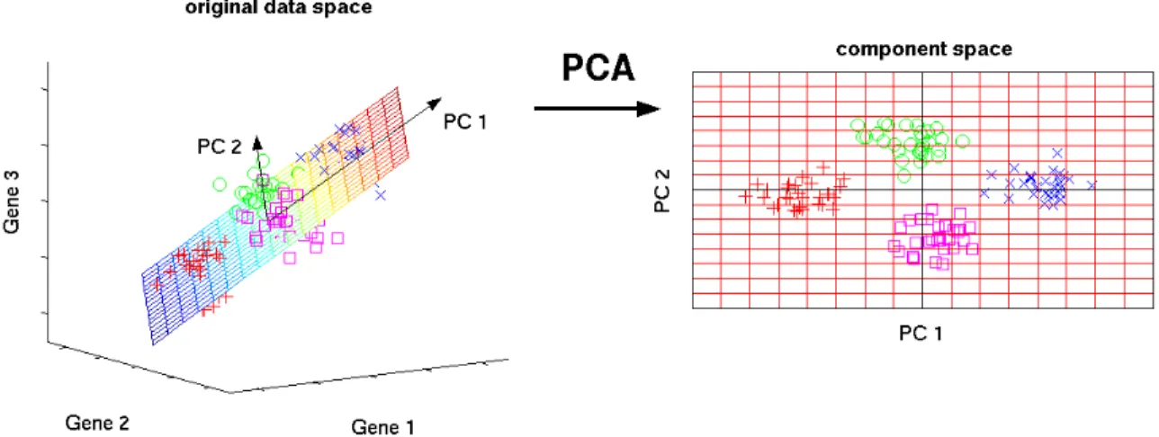
that few ones retain most of the variation present in all of the original variables (see Figure 2.8). More generally, in PCA a few linear combinations which can be used to summarize the data
information, losing in the process as little information as possible. This attempt to reduce
dimen-sionality can be described as “parsimonious summarization” of the information data. For example,
figure2.8shows how a group of trivariate observations is transformed through PCA in other group of bivariate observations in order to get a better interpretation of a dataset.
math-Figure 2.8: An example of how principal component analysis works.
ematical background of population and sample PCA are studied in subsections 2.4.1 and 2.4.2, respectively. Subsection 2.4.3presents a brief discussion about PCA applied on a spatio-temporal raster dataset and finally subsection 2.4.4 discusses about some methods to retain the optimal number of principal components.
2.4.1 Population principal components
Algebraically, principal components are particular linear combinations of the p random variables
x1, x2, . . . , xp. Geometrically, these linear combinations represent the selection of a new
coordi-nate system obtained by rotating the original system with x1, x2, . . . , xp as the coordinate axes.
The new axes represent the directions with maximum variability and provide a simpler and more
parsimonious description of the covariance (or correlation) structure.
Principal components depend only on the covariance matrixΣ(or the correlation matrix ρ) of
x1, x2, . . . , xp, and their development does not require a multivariate normal assumption. Let Σbe
the variance-covariance matrix of the random vectorx0 = (x1, x2, . . . , xp). Let{λ1, . . . , λp}dentote
th eigenvalues ofΣ, such thatλ1 ≥λ2 ≥ · · · ≥λp≥0.
and covariances are given by
V ar(yi) =a0iΣai f or i= 1,2, . . . , p; (2.18)
Cov(yi, yk) =ai0Σak f or i, k= 1,2, . . . , p. (2.19)
The principal components are thoseuncorrelated linear combinationsy1, y2, . . . , yp whose
vari-ances in equation (2.18) are as large as possible.
The first principal component is the linear combination with maximum variance. That is, it
maximizes V ar(y1) =a01Σa1. It is clear that V ar(y1) can be increased by multiplying anya1 by
some constant. To eliminate this indeterminacy, it is convenient to restrict attention to coefficient
vectors of unit length.
Definition 8. Given a set of p random variables x = (x1, . . . , xp)0, the population principal
com-ponents are the variables y1, . . . , yp obtained through the process:
First principal component (y1) = linear combinationa01x that maximizes
V ar(a01x) subject to a01a1 = 1.
Second principal component (y2) = linear combination a02x that maximizes
V ar(a02x) subject to a02a2= 1 and Cov(a01x,a02x) = 0. At the ith step, for i= 3, . . . , p
ith principal component (yi) = linear combination a0ix that maximizes
V ar(a0ix) subject to a0iai = 1 and Cov(a0ix,a0kx) = 0 for k < i.
With this definition, it is possible to get a characterization of the population principal
compo-nents through the eigenvalues and eigenvectors of Σ. The next lemma will help to demonstrate
this characterization.
Lemma 1. Let Bp×p be a positive definite matrix with eigenvalues λ1 ≥ λ2 ≥ · · · ≥ λp ≥ 0 and
associated normalized eigenvector e1,e2, . . . ,ep. Then
max
x6=0
x0Bx
Moreover,
max
x⊥e1,...,ek
x0Bx
x0x =λk+1 (attained whenx=ek+1, k= 1,2, . . . , p−1); (2.21)
where the symbol ⊥is read “is orthogonal to.”
Proof. For details of the proof, see Johnson et al. (2014)
Theorem 1. LetΣbe the covariance matrix associated with the random vectorx0 = (x1, x2, . . . , xp).
Let (λ1,e1), (λ2,e2), . . . , (λp,ep) denote the eigenvalue-eigenvector pairs ofΣ, such thatλ1 ≥λ2 ≥ · · · ≥λp≥0. Then theith principal component is given by
yi =e0ix, f or i= 1,2, . . . , p. (2.22)
With these choices,
V ar(yi) =e0iΣei=λi f or i= 1,2, . . . , p; (2.23)
Cov(yi, yk) =ei0Σek = 0 f or i6=k. (2.24)
Proof. By lemma 1, withB=Σ, gives max
a6=0
a0Σa
a0a =λ1 (attained whena=e1).
But e01e1 = 1 since the eigenvectors are normalized. Thus,
λ1= e01Σe1
e01e1
=e01Σe1 =V ar(y1).
Similarly, using lemma 1again, it follows that max
a⊥e1,...,ek
a0Σa
For the choicea=ek+1 with e0k+1ei= 0, for i= 1,2, . . . , k and k= 1,2, . . . , p−1,
e0k+1Σek+1 e0k+1ek+1
=e0k+1Σek+1 =V ar(yk+1).
However, e0k+1(Σek+1) = λk+1e0k+1ek+1 =λk+1, therefore V ar(yk+1) = λk+1. It remains to show
that if ei andek are orthogonal vectors (fori=6 k) givesCov(yi, yk) = 0. Now, the eigenvectors of Σare orthogonal if all the eigenvalues λ1, . . . , λp are distinct. If the eigenvalues are not all distinct,
the eigenvectors corresponding to common eigenvalues may be chosen to be orthogonal. Therefore,
for any two eigenvectors ei and ek,e0iek= 0 for i6=k. SinceΣek =λkek, premultiplication by ei
gives
Cov(yi, yk) =e0iΣek =λke0iek = 0;
for any i6=k, and the proof is complete.
Due to this characterization of principal components, some observations must be taken into
account. An enumeration of them are shown below:
1. If someλi are equal, the choices of the corresponding coefficient vectors,ei, and henceyi, are
not unique.
2. Principal components may also be obtained for standardized variableszi= (xi−µi)/√σii (i=
1, . . . , p) where µi and σii are the corresponding mean and variance of xi. If so, z =
(z1, z2, . . . , zp)0 would be
z=D−1/2(x−µ); (2.25)
where µ = E(x) and D−1/2 = diag(1/√σii)i=1,...,p. Clearly, Cov(z) = D−1/2ΣD−1/2 = ρ,
which is thecorrelation matrix ofx. Thus, the principal components of standardized variables
are associated to eigenvalues - eigenvectors of its correlation matrix.
in the principal components. It means
p
X
i=1
V ar(xi) = p
X
i=1
V ar(yi). (2.26)
To get this is enough to realize that tr(Σ) =Ppi=1λi.
For a complete review of the PCA methodology and other details see for exampleJolliffe(2002) and Mardia et al. (1980).
2.4.2 Sample principal components
This subsection deals with properties of principal components obtained from a random sample
x1,x2, . . . ,xnrepresentingnindependent drawings from somep−dimensional population with mean
vector µ and covariance matrix Σ. This dataset yields the sample mean vector x, the sample
covariance matrixSand the sample correlation matrixR. The principal components obtained from
the sample covariance matrix (or sample correlation matrix) are calledsample principal components.
The process to obtain the sample principal components is analogous to the population PCA
process but with subtle details. To see this, let
X= (x1 :x2 :· · ·:xn)0; (2.27)
be the data matrix due to the n p−variate observations. As PCA works with the information of variables, a partition of X by columns is necessary. Let X = (x(1) : x(2) : · · · : x(p)) be the matrixXpartitioned by columns, then the sample principal components are defined as those linear
combinations ˆyi =ai1x(1)+ai2x(2)+· · ·+aipx(p) =Xai which have maximum sample variance,
constrained to a0iai = 1. Next definition formalize this concept.
Definition 9. Given a set of n independent observations of p−dimensional random variables,
x1,x2, . . . ,xn, and the data matrix X defined as equation (2.27). Then, the sample principal components are the vectors yˆ1, . . . ,yˆp obtained through the process:
subject to a01a1= 1.
• Second sample principal component: yˆ2 = Xa2 that maximizes the sample variance of Xa2 subject to a02a2= 1 andsample covariance(Xa1,Xa2) = 0.
• At ith step, from i= 3 to p:
ith sample principal component: yˆi=Xai that maximizes the sample variance ofXai subject to a0iai = 1 and sample covariance(Xai,Xak) = 0, k < i.
Theorem 2 solves the optimization problem involved in definition of sample principal compo-nents and gives an explicit characterization of them.
Theorem 2. Let S be the sample covariance matrix associated with a data matrix X= (x1 :x2 :
· · · : xn)0 formed by n independent drawings from some p−dimensional population. Let (λˆ1,eˆ1), (λˆ2,ˆe2), . . . , (λˆp,ˆep) be the eigenvalue-eigenvector pairs ofS, whereλˆ1≥ˆλ2 ≥ · · · ≥λˆp≥0. Then the ith sample principal component is given by
ˆ
yi=Xˆei f or i= 1,2, . . . , p. (2.28)
Also, it follows that
sample variance(ˆyi) = syˆi,yˆi = ˆλi i= 1,2, . . . , p; (2.29)
sample covariance(ˆyi,yˆk) = syˆi,yˆk = 0 i6=k. (2.30)
Proof. The proof is similar as its analogous population PCA process (See theorem 1).
Given the sample principal components structure, it will be convenient to define the matrix of
sample principal components in this way
(ˆy1 : ˆy2:· · ·: ˆyp) = (Xˆe1 :Xeˆ2 :· · ·:Xˆep) =X(ˆe1 : ˆe2 :· · ·: ˆep);
whereZn×p is called the matrix of sample principal components, also known asthe component score matrix, and P the eigenvector matrix of S (o R), also known as the component loading matrix.
From now onwards, the sample principal components and the sample PCA process will be referred
as merely principal components andPCA respectively.
Remark 1. Observe that one can choose either the sample covariance (S) or the sample correlation
(R) matrix to find the principal components. However, in this project the use of sample correlation
matrix is preferred to the sample covariance matrix, because the sample covariance matrix will not
provide very informative principal components if there are variables with widely higher variance
than the others; furthermore, when using the sample covariance matrix it is more complicated to
compare the results from different analyses (Jolliffe, 2002).
2.4.3 PCA in a spatio-temporal context
As it was seen before, PCA maps the originalnobservations of ap−variate population in the data matrixXonto a new orthogonal space, such that the new axes are oriented in directions of largest
variance in the dataset. This structure of dataset is considered traditional data; that is, the n
measurements have a constant and specific position in space and time. So, what would happen if a
PCA is used in a dataset with an explicit space and time structure?, would it be possible to apply
a PCA over a spatio-temporal dataset?, if so, how would the results of a PCA be interpreted?. In
the next paragraphs, a brief analysis of the consequences when using a PCA in a spatio-temporal
dataset is shown.
A review in literature has shown that PCA was applied over a dataset with a space-time
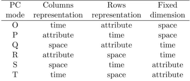
struc-ture, especially in climatology and meteorology fields (see for exampleRichman,1986;Preisendorfer and Mobley,1988). When dealing with spatio-temporal structures three subdimensions need to be considered: temporal, spatial dimension and the attribute (or variable) dimensions, respectively.
According to this, Richman (1986) established six different operational modes of use of PCA to deal with space-time series data: O, P, Q, R, S and T (see table2.1). These modes are classified by having the data matrixXfor PCA defined by two out of the three subdimensions of the space–time
Table 2.1: The six mode of decomposition and how is related to the structure of its respective
data matrix X(equation (2.27)). PC mode
Columns representation
Rows representation
Fixed dimension
O time attribute space
P attribute time space
Q space attribute time
R attribute space time
S space time attribute
T time space attribute
Different modes provide different insight results and interpretations of them (Richman,1986). In particular, for purposes of this project only the S and T modes are of interest. Observe that both
modes work only with one variable which is measured at a specific time position and space raster
location. A brief discussion of the S and T mode in a spatio-temporal raster dataset is carried out
below.
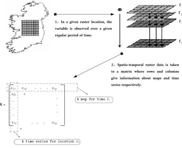
The S mode considers the sampling raster locations as variables and sampling times as data
elements (see figure2.9). Because of this, covariance/correlation matrix is calculated between each pair of sampling raster locations and not between two measured variables as traditional PCA.
Therefore, location does play a role in calculation of the PCs. Also, the data elements are not
more independent and interpretation of PCs must consider this intrinsic temporal characteristic.
Mathematically, consider a bidimensional geographic location given by the latitude and longitude
position. A spatio-temporal raster dataset could be seen as an array containing for each vertical
level a three-dimensional, two-dimensional in space and one-dimensional in time, fieldX. This field is a function of time t, latitude θ, and longitude φ. Suposse that the horizontal coordinates are discretised to yield latitudes θj, j = 1,2, . . . , p1, and longitudes φk, k = 1,2, . . . , p2, and similarly
for time, i.e. ti, i= 1,2, . . . , n. This yields a total number of grid points p=p1p2. The discretised
field reads:
Xijk =X(ti, θj, φk); (2.32)
applying PCA, the field X is transformed into a two-dimensional array: the data matrix X where the two spatial dimensions are concatenated together. Figure 2.9summarizes this process.
t1
t2
t3
tn
X =
1.- In a given raster location, the variable is observed over a given regular period of time.
2.- Spatio-temporal raster data is taken to a matrix where rows and columns give information about maps and time series respectively.
Figure 2.9: Scheme of how the data matrix is obtained when working with a spatio-temporal
raster dataset.
WhenPCAis applied toX, the S mode gives as results the spatial patterns of variability, their
time variation, and gives a measure of the “importance” of each pattern. It finds spatial patterns
of variability because each PC is a linear combination of all locations and a map of its weights
can be produced for each PC. Here the calculated component loadings, of the respective PCs, at
each sampling location are spatially interpolated to form a contour map, which is then inspected
for detecting significant spatial patterns. Next, The PC attached to the corresponding eigenvector
the corresponding proportion of variance explained gives a measure of its “importance” as spatial
variability pattern.
Remark 2. By construction, the eigenvectors of the S mode are stationary structures, i. e. they
do not evolve in time. The PC attached to the corresponding eigenvector provides a simplified
representation of the state of the spatio-temporal field at that time along that eigenvector. In other
words, the eigenvector matrix do not change structure in time, they only change sign and overall
amplitude to represent the state of the measured variable.
On the other hand, working in a T mode gives different insight results. In this case, the sampling
raster locations are considered as data elements and the sampling times as variables. Compared
to the matrix X of the S mode, the T mode would be equivalent to apply a PCA over X0. As a
consequence, the component loadings (eigenvectors) would be time series whereas the PCs would
plot up as a geographical map of PC scores. Therefore, it is expected that the T mode isolates
subgroups of time observations with similar spatial patterns and, thereby, simplify the time series.
This is contrary to the S mode that isolates subgroups of locations which covary similarly.
To end this discussion, what type of mode of decomposition, S or T, would one use? It would
depend on what is the initial goal. For example, if the goal is to get a regionalization of a
spatio-temporal dataset, the S mode would be better. On the other hand, if the aim is to summarize the
information of the time dimension, the T mode would be chosen.
2.4.4 How many principal components to retain?
Up to now, PCA can be seen as a tool that retains meaningful information in the early axes
whereas variation associated to “noise”, measurement inaccuracy, is summarized in later axes.
PCA has the ability to identify relationships by generating linear combinations of variables showing
common trends of variation that can contribute substantially to the recognition of patterns even
in datasets with a space-time structure. However, the issue of determining whether or not a given
axis summarizes meaningful variation (i.e., non-trivial versus trivial components) remains unclear
in many cases.
ith component is the ith ordered eigenvalue corresponding to S (or R). Adding the fact that the sample total variability (trace of sample covariance matrix) fulfills that
Sample total variability =tr(S) =
p
X
i=1
ˆ
λi; (2.33)
then, the contribution of variability corresponding to theith component is given by
P roportion of explained variation byyˆi =
ˆ
λi
Pp
i=1λˆi
!
×100%. (2.34)
Equation 2.34 gives a measure of the “importance” of each component. So, is it of interest to know how many PCs to retain? When the correct number of non-trivial PCs is not retained
for subsequent analysis, either relevant information is lost (underestimation) or noise is included
(overestimation), causing a distortion in underlying patterns of variation/covariation (Ferr´e,1995). Therefore, determining the number of non-trivial principal components is very important because
it provides a meaningful interpretation of multivariate data.
How many PCs are required to adequately explain variance shared by the variables? A variety of
techniques to estimate the number of meaningful components have been proposed (see for example
Jackson,1995;Jolliffe,2002). For example, there exist empirical tests such as Kaiser’s rule (Kaiser,
1960), which takes the number of components that have corresponding eigenvalue greater than +1. Also there exist approaches using simulation such as parallel analysis (Peres-Neto et al., 2005), which replaces the threshold +1 given by the Kaiser’s rule with the mean eigenvalues generated
from independent normal variates through Monte Carlo simulations. Graphical tests that focus on
the elbow of the eigenvalue plot and are not based on a statistical hypothesis test are also found
in literature. These tests are known as the Cattell’s scree tests (Cattell, 1966). These tests are useful and simple, but they do not enable a clear decision-making about the number of components
to retain since the chose depends on the visualization of a graph. To address this limitation, the
scree test optimal coordinate and the scree test acceleration factor are proposed by Raˆıche et al.
this work, the scree test optimal coordinate is chosen due to its simplicity and its better results
(Raˆıche et al.,2013).
Scree Test Optimal Coordinate
This test attempts to determine the location of the elbow by measuring the gradients associated
with eigenvalues and their preceding coordinates. This strategy is done by computing p−2 two-point regression models, and verifying if the observed eigenvalue is, or is not, greater than or equal
to the one estimated by these models. The last of these positive verifications, beginning at the
second eigenvalue, and without interruption of the verification, is used to determine the number
of principal components to retain. In order to make the verifications, two criteria could be taken.
First, following the idea of Kaiser’s rule, as in equation (2.35), or to the location statistics criteria based on the idea of parallel analysis, as in equation (2.36):
noc= p
X
i=1
1{λ
i≥1 &λi≥λˆi}; (2.35)
noc= p
X
i=1
1{λ
i≥LSi&λi≥ˆλi}; (2.36)
wherenocis the number of components retained by the optimal coordinate method, LSi is the
location statistic which is usually given by the 95th quantile of a simulation of eigenvalues from independent normal variates, and ˆλi is referred as the the optimal coordinate. This is obtained
according to linear regression using only the last eigenvalue and the (i+ 1)th eigenvalue as follows:
ˆ
λi =ai+1+i×bi+1; (2.37)
2.5
Autoregressive Neural Network model
The aim of time series analysis is to extract information of a given data series, consisting of
observations over time. This information is used to build a model of the dynamics, called process,
which determines the data series. Such a model can be used for prediction of future values of the
time series. For identification of the process, linear models like linear autoregressive processes (AR)
and autoregressive moving average processes (ARMA) are a standard tool of econometrics (Box and Jenkins,1976). However empirical experience shows that linear models are not always the best way to identify a process and do not always deliver the best prediction results. In this contextGranger et al. (1993) speak of “hidden nonlinearity”, which requires the adoption of nonlinear methods. Since the early 1990’s a lot of nonlinear methods have arisen. They can be divided into parametric
models, characterized by a fixed number of parameters in a known functional form, and the more
general nonparametric models.
The method for nonlinear time series analysis discussed in this section - autoregressive neural
network (AR-NN) model - is parametric. As will be seen later, due to its parametric nature and
ability to approximate any function and therefore any nonlinearity, the AR-NN model is suitable
to analyze time series with non-linear dynamics. Below, subsection2.5.1explains the mechanism of artifical neural networks. Then, subsection2.5.2deals with the theory of autoregressive processes. Finally, subsections 2.5.3and 2.5.4develops the mathematical theory of AR-NN models.
2.5.1 Artificial Neural Networks
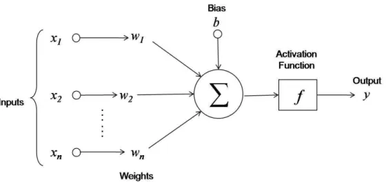
Inspired by biological neural networks, Artifical Neural Networks (ANNs) are groups of
elemen-tary processing units called artificial neurons connected together to form a directed graph. These
elementary processing units are called neurons. Figure 2.10 illustrates a single neuron in a simple neural network model. Nodes of the graph represent biological neurons and connections between
them represent synapses. Unlike in biological neural networks, connections between artificial
neu-rons are not usually added or removed after the network was created. Instead, connections are
weighted and the weights are adapted by learning algorithms.
Chapter 2
Neural Network
In this chapter, we will provide a brief introduction to the neural network
approach. We will start with a general description of the artificial neuron model
and then introduce the topology and the training of the neural networks.
2.1
Processing Unit
A neural network is a set of interconnected neural processing units that imitate
the activity of the brain. These elementary processing units are called neurons.
Figure 2.1 illustrates a single neuron in a neural network.
Figure 2.1: Artificial Neuron Model
In the figure, each of the inputs
x
ihas a weight
w
ithat represents the strength
of that particular connection. The the sum of the weighted inputs and the bias
b
is input to the activation function
f
to generate the output
y
. This process
can be summarized in the following formula:
y
=
f
(
n
X
i=1
x
iw
i+
b
)
(2.1)
A activation function controls the amplitude of the output of the neuron.
Neu-ral Networks supports a number of activation functions: a linear activation
function (i.e.identity function) returns the same number as was fed to it. This
11
Figure 2.10: Artificial Neuron Model.
connection. The sum of the weighted inputs and the bias bare input to the activation function f
to generate the output y. This process can be summarized with the following formula:
y=f
n
X
i=1
wixi+b
!
(2.38)
An activation function controls the amplitude of the output of the neuron. Examples of
acti-vation functions are:
1. Linear activation function (f(x) =x) returns the same number as was fed to it. This is equivalent to having no activation function.
2. Log-sigmoid activation function f(x) = (1 +e−x)−1, sometimes called unipolar sigmoid function, squashes the output to the range between 0 and 1. This function is the most
widely used sigmoid function.
3. Hyperbolic tangent activation function f(x) = eexx+−ee−−xx
, also called bipolar sigmoid function,
is similar to a log-sigmoid function, but it generates outputs between −1 and 1.
5. Hard limit function f(x) =1{x≥0} converts the inputs into 1 if the summed input is bigger than or equal to 0.
12
Chapter 2. Neural Network
is equivalent to having no activation function. A log-sigmoid activation
func-tion (sometimes called unipolar sigmoid funcfunc-tion) squashes the output to the
range between 0 and 1. This function is the most widely used sigmoid function.
A hyperbolic tangent activation function (also called bipolar sigmoid function)
is similar to a log-sigmoid function, but it generates outputs between -1 and 1.
A symmetric saturating linear function is a piecewise linear version of sigmoid
function which provides output between -1 and 1. And a hard Limit function
converts the inputs into a value of 0 if the summed input is less than 0, and
converts the inputs into 1 if the summed input is bigger than or equal to 0.
Figure 2.2 shows these activation functions and their mathematical definitions
can be found in Table 2.1.
−3 −2 −1 0 1 2 3
−3 −2 −1 0 1 2 3
Linear
Symmetric Saturating Linear Hyperbolic Tangent Sigmoid Hard Limit
Log−Sigmoid
Figure 2.2: Activation Functions
Table 2.1: Mathematical Definitions of the Activation Functions
Function
Definition
Range
Linear
f
(
x
) =
x
(-inf,+inf)
Symmetric Saturating Linear
f
(
x
) =
−
1
x <
−
1
x
−
1
6
x
6
+1
+1
x >
+1
[-1,+1]
Log-Sigmoid
f
(
x
) =
1+1e−x(0,+1)
Hyperbolic Tangent Sigmoid
f
(
x
) =
eexx−+ee−−xx(-1,+1)
(
0
x <
0
Figure 2.11: Different types of activation functions.
2.5.2 Autoregressive processes
Definition 10. An autoregressive process (AR, in short) of orderp is defined by
xt=F(Xt−1) +εt; (2.39)
whereXt−1= (xt−1, xt−2, . . . , xt−p)0,F :Rp →R,Xt−1 andεtare independent andεti.i.d.∼ N(0, σ2) (Gaussian white noise assumption).
From definition10, the first term on the right hand side of equation (2.39) is calledthe predictable part, and the second term the stochastic part. Also if F(Xt−1) is a linear function, it is said that
xtfollows a linear AR, but when F(Xt−1) is nonlinear, xt is known as a nonlinear AR.
A linearAR(p) is written as
xt=φ0+φ1xt−1+φ2xt−2+· · ·+φpxt−p+εt. (2.40)
Applications show that in most cases the residuals hardly match the Gaussian white noise
assumption. A linear solution of this problem are the ARMA processes proposed by Box and Jenkins (1976). They assume that the process does not only consist of a linear predictable part and an additive Gaussian white noise. Rather the stochastic part itself may be determined by
a moving average (M A) process of the Gaussian white noise εt. So, an ARM A(p, q) process is
represented by the following equation (q indicates the maximum lag of the MA part):
xt=φ0+φ1xt−1+· · ·+φt−pxt−p+εt+θ1εt−1+· · ·+θqεt−q. (2.41)
Until today ARMA are the most frequently applied process models in time series analysis.
The Wold decomposition theorem (introduced in Wold, 1938) justifies theoretically that one can estimate any covariance stationary process by an ARMA process.
Nonlinear AR models, on its side, try to overcome the problem of observed nonstandard features
(hidden nonlinearity) in linear models. For this purpose, neural networks are able to approximate
any (not specified) function, linear or not, arbitrary accurately. Next subsection links up the neural
networks with a nonlinear AR in a detailed way.
2.5.3 The AR-NN structure
The AR-NN model contains a linear and a nonlinear part. The architecture of an AR-NN model
with one hidden layer is shown in figure 2.12. According to the figure, yellow circles represent the input and output neurons (the variables), the black circle is the bias term (the constant of
the model) and the red lines represent the shortcut weights (parameters) corresponding to the