UNIVERSIDAD NACIONAL DE INGENIERÍA
FACULTAD DE CIENCIAS
TESIS
“DEVELOPMENT IN C++ AND PYTHON OF A TIME
STRUCTURE ANALYSIS TOOL FOR PARTICLE BEAM
ANALYSIS FOR THE MINERvA TEST BEAM EXPERIMENT”
PARA OBTENER EL GRADO ACADÉMICO DE MAESTRO EN
CIENCIAS CON MENCION EN FÍSICA
ELABORADO POR:
GERALD FERNANDO SALAZAR QUIROZ
ASESOR:
Dr. CARLOS JAVIER SOLANO SALINAS
i
ii
Do not go gentle into that good night,
Old age should burn and rave at close of day;
Rage, rage against the dying of the light.
Though wise men at their end know dark is right,
Because their words had forked no lightning they
Do not go gentle into that good night.
iii
Acknowledgments
How can anyone resume all the time, help, advice and support received over
the time that this thesis was done in a couple of lines?. For all of them thanks,
even the tiny hint was useful and well taken. However, there are some important
persons and institutions that I do want to thanks.
To my advisor Dr. Javier Solano for his support and advice during all the time
I spent at Fermilab, as well to Dr. Jorge Morfin: great listener and even greater
physicist. To all the MINERvA Collaboration and specially to Deborah for their
kindest support. From the very first moment in the experiment I was able to see
by myself that science is truly a hard, colaborative and open endeavour in the
pursue of knowledge.
To the Test Beam crew: Leo Bellatoni for all the guidance, Aaron Bercellie,
Rob Fine, Anne Norrick and Geoff Savage, as well to Howard Budd for the
count-less hours teaching me the basis of how to be a Detector Expert. To Edgar
Valencia, from who I receive my first hints in the painful walk of learning ROOT,
which by the way it is not as hard as once appered specially when my code was
crashing even that, minutes before it was working okey. Of course I know the
answer to that: bad use of pointers.
To Paola from who I am still learning a lot of great things. To my 5 Sauk
Circle’s friends: Aaron, Anu, Anna and Maya. During the time I was writing this
thesis my mind was driven gently to the awesome time we spent together, and
iv
Abstract
We present in this thesis the results of the design and programming of a temporal
anal-ysis tool for experiment data MINERVA Test Beam (TbTaTool), which receives pions and
electrons in the energy range corresponding to the end of the interactions of neutrinos
energy states with MINERvA detector. The TbTaTool is independent, flexible and
adapt-able to other contexts where we need to analyze the distribution of events over time,
because it has separated datasets’ production from the tool itself. Our tool has been
applied to the data (Run 2 and Run 3) that the experiment has obtained in MTest at
Fer-milab, focusing on the variables of frequency of spill of the particles (MI’s spill frequency),
duration of spill (MI’s spill duration) and the profile over time of packets corresponding to
the delivery of the particles (time profile). Our calculations show0.01%of difference for the frequency of spill of the particles and9.34%, for the second variable, compared to the values indicated by the Fermilab’s Accelerators Division. Furthermore, this tool had set
the basis for constructing a real time DAQ visualizator of the measurement process.
Resumen
Se presenta los resultados del dise ˜no y programaci ´on de una herramienta de an ´alisis
temporal para los datos del experimento MINERvA Test Beam (TbTaTool), que recibe
piones y electrones en el rango de energ´ıa correspondiente a los estados energ ´eticos
finales de las interacciones de neutrinos con el detector MINERvA. El TbTaTool es
inde-pendiente, flexible y adaptable a otros contextos donde se quiera analizar la distribuci ´on
de eventos respecto al tiempo. Nuestra herramienta ha sido aplicada a los datos (Run 2 y
Run 3) que el experimento ha obtenido en el MTest en el Fermilab, enfoc ´andonos en las
variables de frequencia de entrega de las part´ıculas (MI’s spill frequency), duraci ´on de
la entrega (MI’s spill duration) y el perfil en el tiempo de los paquetes correspondientes
a la entrega de las part´ıculas (Time Profile). Nuestros c ´alculos muestran un 0.01% de diferencia para la frecuencia de entrega de las part´ıculas y9.34%, para la segunda vari-able, frente a los valores indicados por la Divisi ´on de Aceleradores de Fermilab. Adem ´as
esta herramienta ha establecido el fundamento para la construcci ´on de visualizador del
Contents
1 Theoretical Framework 2
1.1 Weak Interactions . . . 3
1.2 Neutrino Physics . . . 7
1.2.1 Solar and Atmospheric Neutrinos . . . 8
1.2.2 Neutrino oscillations . . . 11
2 Neutrino Experiments 14 2.1 Neutrino interaction with matter . . . 15
2.1.1 Intermediate Energy Cross Sections . . . 17
2.2 Neutrino Cross Sections Measurements . . . 22
2.3 Neutrino experiments . . . 25
2.3.1 T2K experiment . . . 26
2.3.2 MiniBoone . . . 27
3 MINERvA a cross-section neutrino experiment 29 3.1 ”Bringing Neutrinos into Sharp Focus” . . . 30
3.1.1 The NuMI Beam at Fermilab . . . 31
3.1.2 MINERvA Detector . . . 32
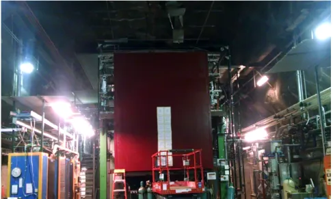
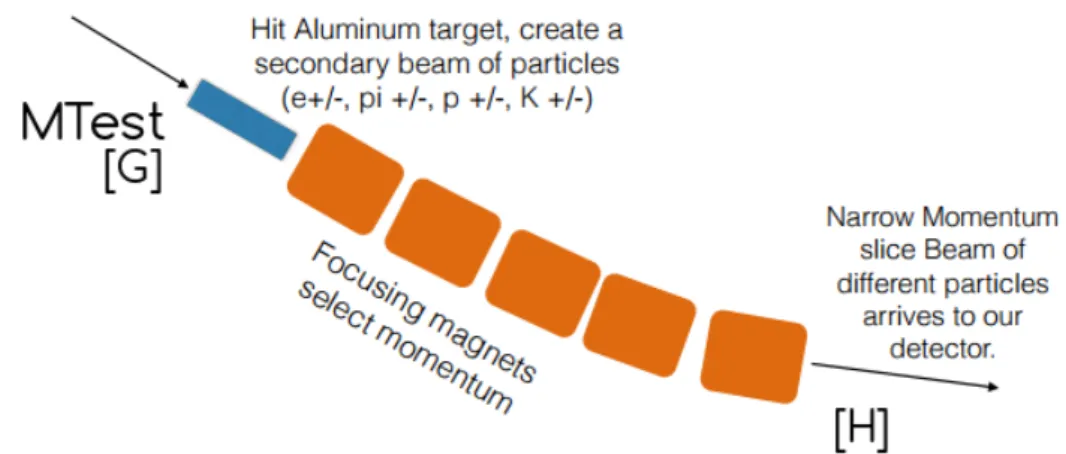
3.2 Test Beam Detector . . . 38
3.2.1 Why is necessary to have a Test Beam program . . . 40
3.2.2 FTBF Beam production . . . 41
3.2.3 Test Beam detector’s auxiliary systems . . . 42
3.2.4 How an event is recorded: trigger logic and DAQ for MIN-ERvA Test Beam 2 . . . 50
CONTENTS vi
4 Time structure of the FBTF Beam 54
4.1 General Concepts in Accelerator Physics . . . 55
4.1.1 Fermilab’s accelerator complex . . . 57
4.2 Radio Frequency Systems (RF Systems) . . . 59
4.2.1 RF Cavities . . . 59
4.2.2 Power Losses in Cavity . . . 63
4.3 Time structure of the Beam . . . 64
4.3.1 Synchronicity condition . . . 64
4.3.2 synchrotron Oscillation, Buckets and Bunchs . . . 66
4.3.3 Time Structure of the Beam at MCenter . . . 67
4.3.4 The Booster and the formation of Buckets and Batchs . . . 68
4.3.5 Main Injector: formation of MI Cycle, Resonance Extraction and Spill frequency . . . 69
5 Tools for Data Analysis 71 5.1 General concepts of Statistical Analysis . . . 72
5.1.1 ROOT: Data Analysis Framework . . . 73
5.2 Description of the Spill scale in the beam at MTest . . . 78
5.2.1 Description of the data . . . 79
5.3 Development and Features of the Time Analysis Tool (TbTaTool) . 80 5.3.1 Election of a reference point in time . . . 82
5.3.2 Number of spills . . . 84
5.3.3 Implementation of the tool for the Test Beam data . . . 86
6 Results 89 6.1 Time profile of the MTest Beam . . . 89
6.2 Main Injector’s Spill Frequency for Run2 and Run3 . . . 93
6.3 Main Injector’s Spill duration at MTest for Pions and Electrons . . . 94
CONTENTS vii
A Auxiliary plots 100
A.1 Spill frequency for only Pions (Run 2) . . . 100
A.2 Spill frequency for Electrons (Run 3) . . . 103
A.3 Spill duration for only Pions (Run 2) . . . 105
A.4 Spill duration for only Electrons (Run 3) . . . 107
B Participation in the MINERνA experiment during 2015 109 B.1 Shifts . . . 109
B.2 Detector Expert Training . . . 111
B.3 PMT Cross Talk problem . . . 112
B.4 PMTs Testings . . . 114
B.5 Data and MonteCarlo Rock Muon eye scanning . . . 115
B.6 Participation in published articles during 2015 . . . 117
C Radiofrequency Cavities theory 119 C.1 Electromagnetic Waves . . . 119
C.1.1 Electromagnetic waves in Vacuum . . . 119
C.1.2 Electromagnetic waves in Matter . . . 121
C.1.3 Electromagnetic Waves in Conductors . . . 122
C.2 Guide Waves and Resonant Cavities . . . 123
C.2.1 Resonant Cavities . . . 126
C.2.2 Power Losses in Cavity: Q of Cavity . . . 129
C.3 ToF basic physics . . . 130
D Documentation of Code 132 D.1 Subroutines . . . 132
D.1.1 Numbers of events in one subrun . . . 132
D.1.2 Numbers of events for a Run . . . 132
D.1.3 Extracting the timestamp of one subrun . . . 133
D.1.4 Extracting the timestamp for the first event of all spills inside one subrun . . . 133
CONTENTS viii
D.1.6 Generation of txt file with timestamps of beginning of the
subrun . . . 134
D.1.7 Matching the two closest timestamps . . . 134
D.1.8 Matching two points for a set of subruns during a data run . 135
D.1.9 Generate a matched times analysis . . . 135
D.1.10 Plotting one variable against all energies of the data set . . 136
D.1.11 Plotting stacked histograms for all energies . . . 136
D.1.12 Plotting one variable for polarities . . . 136
D.1.13 Generating histograms for one variable for all energies and
stacked them in one plot . . . 137
D.1.14 GetValuesHistograms . . . 137
D.1.15 Production of all the analysis . . . 138
E Developed Code 139
E.1 TbTaTool Time Profile (for only one subrun) . . . 139
E.2 TbTaTool Spill Frequency and Spill Duration (for only one subrun) . 148
E.2.1 Cut a variable of time into different parts according to a criteria149
E.2.2 Calculation of different variables regarding time . . . 149
E.3 Auxiliary Tools . . . 150
E.3.1 Tool for match the$39 signal and the corresponding root file 150
E.3.2 Conversion between Unixtime into readable human time . . 151
E.4 Election of the reference point for time profile . . . 153
E.5 Creation of ROOT Files from TXT files . . . 154
List of Figures
1.1 The 2015 Nobel Prize in Physics winners: Takaaki Kajita (left) and
Arthur B. McDonald (right) . . . 4
1.2 Fundamental vertex for weak interactions. . . 5
8figure.caption.7
1.4 (a) Path of the atmospheric neutrinos during its travels through the
earth. (b) Zenith angle events distribution ofe-like andµ-like events in Super-Kamiokande in the range of energy below 1.33GeV[11].
The red line, indicates the best fit for the data points, while the
boxes show the Monte Carlo events expectation considering no
oscillations. . . 10
2.1 Total cross-sections for Charge Current Quasi-elastic Scattering
on Carbon measured by different experiments. This figure has
been taken from the Conference MINERνA 101 by C. Patrick [27] . 16 2.2 Fundamental vertex. This figure has been taken from the
Confer-ence MINERνA 101 by C. Patrick [27] . . . 16 2.3 Total neutrino and antineutrino per nucleon CC cross-sections
di-vided by neutrino energy and plotted as a function of energy. Data
include the low energy data from N ([6]), ∗ ([]), ([]), and ? ([]). The three main regions are ploted as quasi-elastic (dashed),
res-onance production dash), and deep inelastic scattering
(dot-ted). The predicitions for each region are provided by the NUANCE
generator ([7]) . . . 18
LIST OF FIGURES x
2.4 Allνµquasi-elastic scattering cross-sections,νµn→µ−p
measure-ments until the year 2002 by [7] as a function of neutrino energy
for different nuclear targets. . . 20
2.5 Data measurements of νµ CC resonant single-pion production re-ported by experiments with no additional corrections derived of nu-clear targets or invariant mass selections. The continuous curve has been generated by NUANCE. [26]. . . 22
2.6 Absolute coherent pion production measurements from a variety of nuclear targets and samples for NC and CC data [7, p. 33]. . . 23
2.7 Charge Current Neutrino interactions in the intermediate region and the experiments that cover those regions. From M. Martin presented in the NuFact15 [22]. . . 24
2.8 Geographical map of the T2K detection the east coast of Japan. Images from the ofical page of T2K experimenthttp://t2k-experiment. org/. . . 27
2.9 MiniBooNE and MicroBooNE experiments . . . 28
3.1 Front view of the MINERvA detector at NuMI Hall at Fermilab. . . . 30
3.2 Diagram of NuMI and its different elements that produce the neu-trino beam used by MINERvA, MINOS and NOvA experiments. fig. by . Pavlovic. . . 32
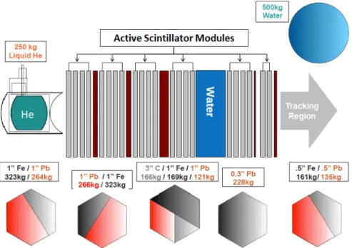
3.3 Side view of the complete detector showing the nuclear target, the active region and the surrounding calorimeter regions. Image[2] . 33 3.4 Active Scintillator Modules, and the 5 types of nuclear modules. Image from A. Norrick [25] . . . 34
3.5 Images form [2] . . . 36
3.6 Images by C.L. McGivern . . . 37
3.7 Typical time slice of . Screenshoot taken on 3/9/16 . . . 37
3.8 Images of the FTBT. . . 39
3.9 Calorimetric response for positive (left) and negative (right) pions for low energies in the Test Beam Program 1 for low energies. . . 40
LIST OF FIGURES xi
3.12 Energies and Polarities taken in the Run 2 and 3. Tables made by
R. Fine. . . 43
3.13 The two configuration for the calorimetric regions in the TB2.
Im-age made by A. Bercelli. . . 44
3.14 (Left) Schematic view of the Test Beam Detector and the Auxiliary
detection System. (Right) Components of the Test Beam and its
functions. . . 44
3.15 (a) TDC-CAMAC Lecroy 3377 used in NuTeV and CDF. . . 47
3.16 Veto system and its six paddles. Photo by A. Norrick . . . 47
3.17 Time of Flight Upstream and Downstream detectors. Photos by A.
Norrick . . . 48
3.18 A diagram of the Cerenkov detector used at MTest (Fermilab).
Copyright Fermilab. . . 49
3.19 Spectra of de Cerenkov detectors at MTest for the MINERvA
Ex-periment. Work done by M- Ramirez . . . 50
3.20 Underground trigger timing with the MINERvA Main Detector. . . . 51
3.21 Underground Trigger timing within the Test Beam Detector. . . 52
3.22 Logic of the triggers in the Auxiliary Test Beam detectors. . . 53
4.1 Fermilab Accelerator Complex. . . 58
4.2 A niobium-based 1.3 GHz nine-cell superconducting radio frequency
to be used at the main LINAC of the International Linear Collider.
Photo from FNAL. . . 60
4.3 A pillbox cavity. The lower mode frequency does not depend from
the height of the cavity. . . 62
4.4 The resonance curve’s full width is equal to the central frequency
ω0 dived byQ. . . 64
4.5 Graphic description of a Bucket and a Bunch, the RF voltage that
the particles see while they are in a bunch and how the buckets
arrange themself on a synchrotron’s ring. . . 67
LIST OF FIGURES xii
4.7 Diagram showing the MI’s cycle formation, spill duration and spill
frequency. . . 70
5.1 A standardd histogram with box plots generate in ROOT. . . 73
5.2 Structure of the data in a ROOT file. . . 74
5.3 Fitting a histogram made with three lines of code. . . 75
5.4 Structure of the data in a ROOT file. The comments below the plots are the ROOT commands. . . 77
5.5 Diagram of how the data is ordered in the ROOT file. The variable shown isTime of readout. (a) and (c) are the energies that Run 1 contains for electrons and pions in both polarities (all the energies are presented in tab. 5.1). (b) Run 2 and Run 3 contain onlu electrons and pions. (d) Each Run has a number of subruns. (e) Each subrun constains the the data for 1000 gates or events. (f) One of the variables is theT imevariable as shown in this figure. . 80
5.6 Bias in the time profile by using an internal reference point mea-sure in seconds. As can be seen, the (b) elecction allow us to reduce the lost of events between the zero point and the first event. 82 5.7 Distribution of the values of the interval between the first event recorded (kickoff od the spill) and two reference points: the $39 signal and the beginning of the subrun. . . 83
5.8 File that contains dates from the signal$39as a reference point. . 84
5.9 Number of spills for Run 2 and Run 3. . . 85
5.10 MI’s Spill frequency during May 2015. Infor provided by A.D. . . 86
LIST OF FIGURES xiii
5.12 From (a) to (e) apply to one subrun. (b) the different points of
reference in order to get the time profile. (c) and (d) explain how
the spill duration and the spill frequency are calculated. When the
calculation for one subrun is done, the next is calculated until the
last sunrun. (f) and (g) describe how all of them are stacked and
plot (i) and (j) according to different variables (h). . . 88
6.1 Time profile for Run2±4,±6 and±8 GeV (pions). . . 90
6.2 Time profile for Run2±9,±10 and 16GeV (pions). . . 91
6.3 Time profile for Run3±2,±4,±8, 3 and 5GeV (electrons) . . . 92
6.4 Spill frequency for Pions (a,b) and Electrons (c,d). Pions have en-ergies of 4, 6, 8, -8, 9, -9, 10 and 16 GeV, and electrons 2, -2, 4, -4, 8, -8, 3 and 5 GeV . . . 93
6.5 Spill duration for all Runs (a,b) and Electrons (c,d). Pions have energies of 4, 6, 8, -8, 9, -9, 10 and 16 GeV, and electrons 2, -2, 4, -4, 8, -8, 3 and 5 GeV . . . 94
6.6 Errors against the oficial values of the MI’s frequency spill and MI’s spill duration. . . 95
A.1 Spill frequency for 4GeV Pions . . . 100
A.2 Spill frequency for 6GeV Pions . . . 100
A.3 Spill frequency for 8GeV Pions . . . 101
A.4 Spill frequency for 9GeV Pions . . . 101
A.5 Spill frequency for 10GeV Pions . . . 101
A.6 Spill frequency for 10GeV Pions and all the events . . . 102
A.7 Spill frequency for 2GeV electrons . . . 103
A.8 Spill frequency for 4GeV electrons . . . 103
A.9 Spill frequency for 3GeV and 5GeV electrons . . . 103
A.10 Spill frequency for (±)8GeV and all energies electrons. . . 104
A.11 Spill duration for data set containing only pions (Run2). . . 105
A.12 Spill duration for data set containing only pions (Run2). . . 106
A.13 Spill duration for data set containing only pions (Run2). . . 106
LIST OF FIGURES xiv
A.15 Spill duration for electrons (Run3). . . 107
A.16 Spill duration for electrons (Run3). . . 108
B.1 (a) Left. Run Control of the MINERvA Main Detector. (b) Right.
Near MINOS DAQ, not all information is useful for MINERvA, just
the two bottom columns.) . . . 110
B.2 (a) Up left. NuMI Beamline Status Display which shows the status
of the beam. (b) Up right. MINERvA Veto Wall control. (c) IF
Beam Data Server A9 event monitoring. (d) Bottom left. MINERvA
Quality Checklist. (e) Bottom right. Live event display for neutrino
interactions in the Main Detector. . . 111
B.3 Diagram of the MINERvA DAQ System. The Detector Expert
train-ing include a deeper knowledge in these areas. . . 112
B.4 Cross Talk tasks . . . 113
B.5 (a) Left. Some photos the Sillicon Detector Facility and the
equip-ment where the PMTs’ tests were done. (b) Right. Run and Slow
Control and some histograms which confirmed the presence of
cross talk. . . 114
B.6 Monte Carlo simulated Rock Muon interaction with the detector. . . 115
B.7 Real interaction of Rock Muons with the detector. . . 116
C.1 Examples of wave guides. . . 123
C.2 A pillbox cavity. The lower mode frequency does not depend from
the height of the cavity. . . 127
C.3 The resonance curve’s full width is equal to the central frequency
List of Tables
1.1 Range of interaction of the four fundamental forces. . . 6
1.2 Sensitivity of different oscillation experiments.[32, p. 11] . . . 12
2.1 Experiments focus on cross-sections and oscillation of neutrinos and the type of channels of interaction focus on. . . 25
2.2 Neutrino experiments and their localizations. . . 25
2.3 Experiments and their detection technology. . . 26
3.1 Modes of operation of the CAMAC 3377 TDC. The ? means that there is no information . . . 46
3.2 Lowest momenta value for detection in Cerenkov detectors at MTest (Fermilab) . . . 49
4.1 Time structure of the Beam according to Accelerator Division. . . . 67
5.1 Configurations of the Test Beam detector and the type of particles that contain them. . . 79
5.2 Number of events for Run2 and Run 3 considering all the spills, equal to 10, 6 or 2 spills per subrun. . . 84
D.1 Calculation of the number of events in one subrun. . . 132
D.2 Calculation of number of events for a set of root files. . . 133
D.3 Getting the unix timestamp for one subrun. . . 133
D.4 Getting the unix timestamp for the beginning all the spills in one subrun. 133 D.5 Return one timestamp for the real beginning of one subrun. . . 134
D.6 Function that create a txt file with beginning timestamps of root files. . . 134
D.7 Function that matches a set of two points. . . 135
LIST OF TABLES xvi
D.8 Function that matches a set of two points for various root files. . . 135
D.9 Function that generate the plots that shows the interval between all the matched points. . . 135
D.10Function that plots the histograms of one variable. . . 136
D.11Plotting stacked histograms for all energies . . . 136
D.12Plotting one variable for polarities . . . 137
D.13Generating histograms for one variable for all energies and stacked them in one plot . . . 137
LIST OF TABLES xvii
Introduction
In Chapter 1, a theoretical review of weak interactions is done in order to describe the weak sector of the Standard Model (sec. 1.1) and introduce the
neutrino oscillation research (sec. 1.2). By now we know that the deficit in the
solar and atmospheric neutrinos reaching the earth is due to neutrino non-zero
mass which express in neutrino flavour oscillations. However in order to confirm
the value of masses between the three neutrinos more precise experiments are
needed in the reduction of systematic erros due to neutrino interactions with the
detectors. This is the motivation of the neutrino experiments like MINERvA Chap-ter 2 and 3. The improve of detection models between neutrinos and nucleus, since modern experiments are and will rely more on heavy nucleus detectors like
argon or lead. The calorimetric response and the fine detection of last product
pi-ons by the detector allows to recpi-onstruct the incoming neutrino energy. MINERvA
face this challenge by setting up a small scale replica detector called Test Beam
Detector Chapter 4 where we receive particles of knwo momenta and type in order to improve the models detection of pions, muons and electrons of the main
detector.
But, as important of knowing the composition of the beam, it is important to
know the time structure of it, in order to set up timing resolution of your detection
system. That is what this analysis has carried out, a comprobation of the timing
in the scale of Main Injector time space: the spill. In Chapter 4 and Appendix Ca review of the Time Structure of the Beam and the Electromagnetic theory of Radio Frequency Cavities are stated. Section 4.3 describe why the beam that we
received have a specific structure in time.
InChapter 6, we describe the Analysis Tool developed in C++ and ROOT that allow us to analysis the scale of spill. Its features and how the tool works close
that chapter. Finally in Chapter 7, Appendix A and Chapter 8 we present the results and conclusions fo this work.
I must mention that I had a small contribution in two publications of MINERvA:
LIST OF TABLES 1
T´ıtulo: Charge pion production in interactions on hydrocarbon at <E>!= 4.0GeV
Autores: G. Salazar, A. Zegarra, C. J. Solano Salinas and the MINERvA Colab-oration
(b) Physical Review Letters Vol 116 (2016) 081802
Title: Measurement of Electron Neutrino Quasielastic and Quasielasti-clike Scattering on Hydrocarbon at<E>!= 3.6GeV
Authors: G. Salazar, A. Zegarra, C. J. Solano Salinas and the MINERvA colab-oration)
Finally in Appendix B, a review of other activities during the intership at
Fermi-lab has been described. In theAppendix Dwe present the documentantion and in Appendix Ethe parts of the code. The final tool can be found in a public repository at github1.
Chapter 1
Theoretical Framework
One of the greatest achievements in science, is the formulation of the Standard
Model of Particle Physics, a quantum field theoretical framework which has the
most complete description of the fundamental process in nature.
As a quantum field theory, the Standard Model (SM) has been formulated in
terms of Lagrangians, with three fields: Gauge fields (bosons of spin 1 whose
mediate forces), Weyl fermions (which outline massless neutrinos) and a spin 0
scalar field which describe the Higgs boson. These SU(3)xSU(2)xU(1) gauge
fields portray what types of particles and interactions are allowed, where the
SU(3) gives rise to the strong interactions, SU(2) and U(1) describe the weak
and electromagnetic interactions.
The success of this model, has been stated because the predictions of new
phenomena and particles in a very precise way while the technology started to
reach the values of energies required. For example: in 1974, the discovery of
the J/psi (c quark); in 1977, the b quark; in 1981/82, W+- and Z bosons were
discovered. The appear of the Higgs boson in 2012 is probably one of the most
important milestones achieve by the Standard Model.
But, as impressive the predictions of the SM are, also the gaps and new
find-ings that do not fit in the theoretical framework. The baryon asymmetry of the
Universe ([23, p. 9]), the identity of dark matter, for how long the proton lives? or
the neutrino’s masses are a couple of flags inside the model. It is the neutrino
oscillations and the related neutrino cross-section scattering research that give
CHAPTER 1. THEORETICAL FRAMEWORK 3
experiments like MINERνA the fuel to look deeper into the nature of interactions of neutrinos with matter.
One of the most impressive feature of the neutrino is that is not massless,
in contradiction with the Standard Model. Neutrinos research is one of the most
interesting, growing and intensive area of research in particle physics, with
fu-ture experiments that involve billions of investment as is the case of the DUNE
experiment.1 2
It is worth to mention that the 2015 Physics’ Nobel Prize went to T. Kajita
and A. McDonald for the neutrino’s oscillations research in Super-Kamiokande
(Japan) and the SNO Experiment (Canada) (fig. (1.1)):
”For the discovery of neutrino oscillation which shows that neutrinos
have mass”3
Other neutrino Nobel Prizes have been awarded in 1988to L. M. Lederman, M. Schwartz and J. Steinberger ”for the neutrino beam method and the
demon-stration of the doublet structure of the leptons through the discovery of the muon
neutrino”; in1995to M. L. Perl ”for the discovery of the tau lepton” and F. Reines ”for the detection of the neutrino”; in 2002 to R. Davis Jr. and M. Koshiba ”for pioneering contributions to astrophysics, in particular for the detection of cosmic
neutrinos” and R. ”for pioneering contributions to astrophysics, which have led to
the discovery of cosmic X-ray sources”4. For sure, those Nobel Prizes will not be
the last one to be awarded to neutrino research.
1.1
Weak Interactions
Decays ofµandτ decays’ and natural radioactivity are due to weak interactions. Even that unified weak and electromagnetic theory was proposed by S. Weinberg
1The Deep Underground Neutrino Experiment (DUNE) is a proposed experiment with a near
detector at Fermilab and a far detector at the Sanford Underground Research Facility at South Dakota. This international mega-science project is designed to discover, for example, if neutrinos exhibit matter-antimatter asymmetries. More information athttp://www.dunescience.org/
2Ghosh, Pallab (15 February 2014). ”UK backs huge US neutrino plan”. BBC News. Retrieved
15 February 2014.
3http://www.nobelprize.org/nobel_prizes/physics/laureates/2015/
4The quotations have been reviewed from the official page of the Nobel Prize Foundation
CHAPTER 1. THEORETICAL FRAMEWORK 4
Figure 1.1: The 2015 Nobel Prize in Physics winners: Takaaki Kajita (left) and
Arthur B. McDonald (right)
and A. Salam in the late sixties, the actual discovery of the mediators did not
happen until January of 1983.
During the decade 1964-1974 ([16, p. 42]), the particle physics theoretical
framework was incomplete and full of new discoveries that did not fit on it. In the
summer of 1974, the ψ meson was first observed at Brookhaven Laboratory by a group under C.C. Ting, with a lifetime of 1000 times greater than any particle;
by next year it was a new lepton: the tau[30]. In 1983, theW was discovered by Carlo Rubbia’s group at CERN5(at81±5GeV /c2and five months after, theZ0 (at 95±3GeV /c2)6.
Now we know that matter is made out of three kind of elementary particles:
leptons, quarks and mediators. There are three generations of leptons, according
to their charge (Q), electron number (Le), muon number (Lµ) and tau number (Lτ),
each of these numbers define a generation or a family, composed by a lepton and
its corresponding neutrino. The classification ends considering the particles and
antiparticles, the weak force having two mediators for charge currents (W±) and one for neutral current (Z0).
These three mediators (W±, Z0) correspond to the triplet for SU(2)L and a
single, forU(1)Y The symmetry breaking in theSU(2)L×U(1)Y sector gives the
5G. Arnison, Physics Letters B, Volume 122, Issue 1, 1983, Pages 103-116.
6G. Arnison, UA1 Collaboration. Physics Letters B, Volume 126, Issue 5, 1983, Pages
CHAPTER 1. THEORETICAL FRAMEWORK 5
three SU(2) mediators mass thought the interactions with the Higgs Boson. The
photon, though stay massless.
Since the three mediators have positive, negative and no charge, the
inter-actions can be ordered into charged currents interinter-actions and neutral currents
interactions.
The fundamental charged vertex is presented in the fig. (1.2). A neutrino is
produced by its corresponding lepton, with the emission of a W− (or absorption ofW+)
Figure 1.2: Fundamental vertex for weak interactions.
A more complicated reactions can be produce if the primitive diagram is
com-bined, as for example for the reactions:
µ−+νe →e−+νµ
¯
νe+p→n+e+
(1.1)
If the target is a nucleon and with the necessary energy of the income
neu-trino, we can resolve the nucleus as a one (CCQE - Quasielastic Interactions) or
as a quarks (DIS - Deep Inelastic Scattering). For example, the reaction (1.1)
is called inverse neutron decay and was used by C. Reins and F. Cowan in the
discovery of the antineutrino. Also, weak charged current can change lepton and
quark flavours.The fundamental neutral current (fig.2.2) was first suggested in
1958 by Bludman7, that preserves the three leptonic numbers.
The 1973 CERN’s bubble chamber, revealed that in the reaction ν¯µ+e− →
¯
νµ+e−, a neutralZ0was the mediator8. The same experiment saw the mediation
7C. D. Anderson. ”Early Work on the Positron and Muon ” American Journal of Physics
De-cember 1961 Volume 29, Issue 12, pp. 825
CHAPTER 1. THEORETICAL FRAMEWORK 6
of this boson in neutrino-nucleon scattering (1.2), with values of three times large
as those related with charged events [16, p. 323].
νµ+N →νµ+N (1.2)
From the values of decay lifetimes we can be inferred the forces that produces
and the strength of the interaction. Pions and muons decays’ lifetimes (1.3) are
considerably longer than particles that decay only by strong and electromagnetic
forces. The difference in the order of magnitudes are evidence of the existence
of another type of interaction, beside the strong interaction.
π− →µ−ν¯µ, withτ = 2.6×10⁻⁸sec,
µ−→− ν¯eνµ, withτ = 2.2×10⁻⁸sec, (1.3)
Finally we recall that the lifetimes are inversely related to the coupling strength
of this interactions, that means that this new interaction is has weaker coupling
than electromagnetism.
Table 1.1: Range of interaction of the four fundamental forces.
Interaction Range Lifetime Cross Section Coupling
(sec) (mb) αi
Strong 1F' 1
mπ 10
−23 10 1
Color
confinement e.g. ∆→pπ e.g. πp→πp
range
Electromagnetic ∞ 10−20∼10−16 10−3 10−2
e.g.,π0→γγ e.g.,γp→pπ0
Σ→Λγ
Weak MW1 10−12or 10−11 10−6
with longer
MW '100mp e.g.,Σ−→nπ− e.g.,νp→νp
π−→µ−ν¯ νp→µ−pπ+
CHAPTER 1. THEORETICAL FRAMEWORK 7
1.2
Neutrino Physics
Neutrino was proposed by Wolfgang Pauli in 1930 to hold up the energy-momentum
conservation law and Fermi’s statistics inβ-nuclei decay (eq. 1.4). This new par-ticle had to have: no charge, should not interact with matter, or in the other case
interact very weakly and almost no mass. For the same problem Bohr, proposed
a statistical version of the energy conservation law. Experiments showed that
Pauli was right.
n0 →p++e−+ ¯νe (1.4)
In 1932, a more massive neutral particle was discovered by Chadwick([8]),
and was named neutron. Pauli’s name of the unknown particle was turned into
neutrinos (little neutron one) by Enrico Fermi, who used it in 1932.
In 1956, the antineutrino was discovered experimentally by F. Reines an C.L.
Cowan allowing the interaction of protons with electron antineutrinos’ fluxes9
cre-ated in nuclear reactions (eq. 1.5):
¯
νe+p+→n0+e+ (1.5)
The detection was made since a positron quickly finds an electron producing
two opposite 0.5 MeVγrays which are detectable, but not necessarily the indica-tion of the antineutrino existence. Another gamma ray is detected due to capture
of the neutron by the nucleus (n+108Cd→109Cd∗ →109 Cd+γ). This two events
configure the signature of an antineutrino interaction looked.
Neutrinos are elementary particles with spin1/2, electrically neutral and obey Fermi-Dirac statistics. The Standard Model consider threeWeyl massless neu-trino flavors: νe, νµ, ντ, each one corresponding to three different leptons, the
electrone−, the muonµ−and the tauτ, each doublet has their antiparticles. However the nature of neutrino is still open, for sure they are not Weyl’s
mass-less fermions. Two plus one options arise: neutrinos can be Majorana neutrinos,
CHAPTER 1. THEORETICAL FRAMEWORK 8
Figure 1.3: Schematic diagram of neutrino detector as appeared in the original
paper of Reines and Cowan10.
Dirac neutrinos or a mix between both where the seesaw mechanics plays an
important role.
Parity and CP invariance
Parity is violated in weak interactions as Goldhaber observed, neutrinos have spin
antiparallel to their momentum (left-handed) and antineutrinos have it parallel
(right-handed).11
Not only the parity is violated, but also the charge conjugation invariance,
whereΓis the lifetime of process. For instance,
Γ(π+→µ+νL)= Γ(6 π+ →µ+νR) P violation,
Γ(π+ →µ+νL)6= Γ(π−→µ−ν¯L) C violation,
(1.6)
but the CP variance is conserved. Future experiments have as main objective
the comprobation of the CP invariance or its violation by neutrinos.
Γ(π+ →µ+νL) = Γ(π−→µ−ν¯R) CP invariance. (1.7)
1.2.1
Solar and Atmospheric Neutrinos
Theneutrino mass, is one of the most important discoveries from the last decade outside the framework of the Standard Model12.
11 The historic experiment for testing this, was with β-transitions of polarized cobalt nuclei. 60C→60N i∗+e−+ ¯ν
e
CHAPTER 1. THEORETICAL FRAMEWORK 9
Solar Neutrinos
The Solar Neutrinos problem was first formulated in 1964 by Ray Davis’s and
John N. Bahcall from the Homestake Experiment13, who were the first to look
a deficit in the flux of neutrinos from the Sun. Their final results, published in
1998[10], showed that the experimental value,2.56±0.16(stat) ±0.16(sys) was over30%of the theoretically flux value8.5±0.9SNU [28].14
So why the experimental flux that reaches the earth is anomalously low? This
is the core question of the Solar Neutrino Problem[1, p. 10].
We are able to distinguish the solar neutrinos, since we know the sun’s
pro-cesses that generate them: fusion of hydrogen to helium: p+p →2H+e++νe,
the pp-chain4p→4 He+ 2e++ 2ν
e and the CNO-cycle are process that produce
neutrinos[21, p. 9-7].
While measurements of the different solar neutrinos’ chains were improved,
in the flux did not change. The Sudbury Neutrino Observatory (SNO) with a
Cerenkow detector of 1000ton ultra-pure heavy water (D2O) in an acrylic sphere
of 12 m diameter, clearly state that the deficit was not a technical problem,
in-stead the conversion betweenνe andνµ was a physical event, later confirmed by
KamLAND reactor experiment.15
Atmospheric neutrinos
As we know, cosmic rays from outer space interact with the atmosphere
generat-ing particles that come into the earth’s surface. Through these decays processes
(eq. 1.8), we are able to study the flux atmospheric of electron and muon
neu-trinos putting the detectors underground, shielding them from the muons and
electrons generated.
13A lot of information about the experiment and the papers can be found on the web page
http://www.nu.to.infn.it/exp/all/homestake/
14A SNU is the solar neutrino unit (SNU). It is equal to the neutrino flux producing10−36 cap-tures per target atom per second.
15As mentioned before, with the Super-Kamiokande Collaboration won the 2015 Physics Nobel
CHAPTER 1. THEORETICAL FRAMEWORK 10
π± →µ±+νµ( ¯νµ)
µ± →e±+νe( ¯νe) + ¯νµ(νµ)
(1.8)
At low energies (≤ 1GeV), the ratio between the flux of muon-neutrinos to electron-neutrinos was around∼2[15]16. A better ration index was later improved
definingR as the ratio of data to theoretical expectation fluxes. The IMB experi-ment17 reportedR ∼0.54[19] and KamiokandeR ∼0.60[18].
Later, T. Kajita from Super-Kamiokande experiment18 presented compelling
evidence in favour of neutrino oscillations in the neutrino conference Neutrino’98[14].
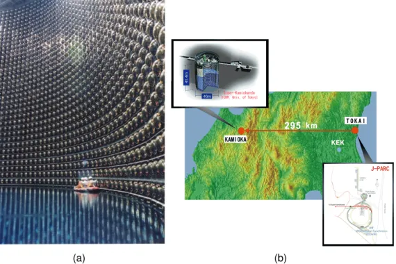
(a) (b)
Figure 1.4: (a) Path of the atmospheric neutrinos during its travels through the earth. (b) Zenith angle events distribution of e-like and µ-like events in Super-Kamiokande in the range of energy below 1.33GeV[11]. The red line, indicates the best fit for the data points, while the boxes show the Monte Carlo events expectation considering no oscillations.
If the flux of neutrinos coming from the atmosphere is expected to be isotropic,
independent of the zenith, a question raised, why the observed fluxes of up-going
16The ratio is defined asR= (N
µ/Ne)DAT A/(Nµ/Ne)M C
17The Irvine-Michigan-Brookhaven Water-Cerenkov detectors (Ohio, USA) http:
//www-personal.umich.edu/~jcv/imb/imb.html
18Super-Kamiokande Collaboration a 50000t water Cerenkov detector, 10 times larger than its
CHAPTER 1. THEORETICAL FRAMEWORK 11
and down-going neutrinos in an underground detector are not the same?. While
the flux ofe-neutrinos has almost no zenith angle dependece (right plots from fig. 1.4), theµ-neutrinos’s flux of down-going (cosθ = 1) exceeds the flux of up-going
νµ.
The most simple explanation was accepted: neutrino flavour oscillation.
Neu-trinos moving upward through the detector are created in the atmosphere at the
opposite side of the Earth, and travel thousand of kilometers before interaction.
Apparently muon-neutrinos disappear on the way whereas electron-neutrinos
do not. Down-going muon-neutrinos, produced in the atmosphere directly above
the detector, only travel a few dozen kilometers and are detected at the level
expected. No indication of an increased electron-neutrino flux, the missing
muon-neutrinos must have oscillated into tau-muon-neutrinos.
After 1998, neutrino oscillations started to open a new set of question that
needed to be answered through the design of new experiments focus on neutrino
oscillations, and as we will mention, a shears experiments started to work in the
improvement of the models of neutrino-nucleus interaction, like MINERνA (sec. 3.1). In the next section, a brief review of the oscillation of only two flavours are
made.
1.2.2
Neutrino oscillations
Consider for simplicity that two of the known neutrinosνe andνµ are eigenstates
with no well defined masses but they are a linear composition of the neutrino mass eigenstatesν1 andν2 with massesm1 andm2, respectively:
|νei=|ν1icosθ+|ν2isinθ
|νµi=−|ν1isinθ+|ν2icosθ,
(1.9)
whereθis the neutrino mixing angle. We will get the dependece of the oscilla-tion probability with the energy and the difference of masses. Following the rules
of quantum mechanics, we can construct the state at any time t, and then get the
probability of transformation from a state to another.
CHAPTER 1. THEORETICAL FRAMEWORK 12
|ν(0)i = |νµi , the propagation of this state in time is dictated by the free
non-time dependent Hamiltonian.
|νti=−|ν1ie−iE1tsinθ+|ν2ie−iE2tcosθ, (1.10)
whereE1,2 =
q
p2+m2
1,2 ≈p+
m2 1,2
2p . The probability of finding a neutrino with
electron flavor is then:
P(νµ →νe;t) = |hνe|ν(t)i|2
=sin2θcos2θ| −e−E1t+e−iE2t|2 =sin22θsin2(∆m
2t 4E )
=sin22θsin2(∆m 2L 4E )
(1.11)
Here ∆m2 = m2
2 −m21 is the squared mass difference and E = p. The last
line is valid for relativistics particles (L = t) with L being the traveled distance, which in practice allow us to construct tunels of decays in order to observe the
oscillation, or in turn place the far and near detector in an oscillation experiment
at a fixed distance.
As it can be seem the mass difference is present in the form of a squared
difference, hence the measuring oscillation probabilities will not give absolute
values of the masses. In the table (1.2), different sources of neutrinos and the
minimum value that can reach the measurement of min(∆m2)[eV2].
This model with two flavors, can be extended to one with three flavor mixing
and three angles, three squared massess differences ∆m2
12, ∆m213 and ∆m223.
[20]
CHAPTER 1. THEORETICAL FRAMEWORK 13
Source Type ofν E[MeV] L[km] min(∆m2)[eV2]
Reactor ν¯e ∼1 1 ∼10−3
Reactor ν¯e ∼1 100 ∼10−5
Accelerator νmu¯ , νµ ∼103 1 ∼1
Accelerator νmu¯ , νµ ∼103 1000 ∼10−3
Atmosphericν’s’ ν¯e,µ,νµ,e¯ ∼103 104 ∼10−4
Chapter 2
Neutrino Experiments
In recent years, many experiments1have been setup in order to improve the
mod-els of interaction between detectors and neutrinos due to requirement of neutrino
oscillation experiments.
Neutrino interaction’s models need to predict not only the signal and
back-ground of mass neutrino oscillation, but also how the energy is transfered to the
observable particles, while reducing the uncertainties2. As mentioned by D. Har-ris: [17, p- 1]
”Future oscillation experiments such as DUNE [9] depend on the ability to
predict far detector signal’s (background) spectra at the 1% (5%) level (...), the
particle physics community is still at the level of measuring cross sections and
making far detector predictions at the7−10%level.”
New oscillation experiments need to expand the models for other nucleus
than hydrogen or deuterium, since the far and near detectors are made of targets
of carbon, water, argon or iron. Another requirement for neutrino cross-section
experiments is to focus energy region of few hundred MeV to a hand full of GeV,
since oscillation probabilities are function of the inverse of the neutrino energy.
It is worth to mention that MINERνA has a15%constrain from a CCQE mea-surements and10%in the flux uncertainties ”[17].
1Only for mention some of them: MINERνA, T2K (Tokai to Kamioka), NOνA, MINOS and
MicroBooNE
2Another source of uncertainty comes from the incoming neutrino flux which is now at8%to
10%.
CHAPTER 2. NEUTRINO EXPERIMENTS 15
MINERνA3is a cross-sections precision studies experiment of
(anti)neutrino-nucleus scattering in the range of 1-20GeV at the NuMI Beam at Fermilab. The
tracking region is made purely by scintillators which recognize the particle by
the energy loss per unit length (dE/dx) after the neutrinos had interacted with the targets (carbon, iron and lead) interleaved between the scintillator planes.
Technical details of the experiment will be describe in sec. 3.1.
This chapter state the principal concepts of neutrino interactions with
mat-ter (sec. 2.1), the different regions of cross-section inmat-teraction ν-A regarding the energy (sec. 2.2) and experiments that perform measurements of neutrino’s
properties (sec. 2.3).
2.1
Neutrino interaction with matter
The cross-section (σ) quantify the interactions between particles and targets, re-garding energy, flux and type of interactions taking place (if it is a strong,
electro-magnetic or a weak interaction).
Defined as the rate (sec. 2.1) of interactions between incoming particles that
are scattered due to the interaction with the targets over a known energy and flux
of incoming particles,
σ= Number of reactions of a given type per unit time
(Incoming flux)(Number of target particles) (2.1)
σ is a number that has dimensions of area and is usually expressed in cm2 or
in barns (1barn= 10−24cm2)45.
Differential cross-sections(dσ/dA) is a distribution of probability, which give us the dependence of the cross-sections to an specific variable (A), for example the angle rangedθ around some direction θ.
Anelastic cross-sections, is a type of interaction where neither beam parti-cle or the target has been disintegrated, the opposite is called aninelastic
cross-3Main INjector ExpeRimentν-A
4The proton-proton cross-sections is 40mb
5For each cross-section corresponding to a particular type of interaction, the term partial is
CHAPTER 2. NEUTRINO EXPERIMENTS 16
Figure 2.1: Total cross-sections for Charge Current Quasi-elastic Scattering on
Carbon measured by different experiments. This figure has been taken from the Conference MINERνA 101 by C. Patrick [27]
Figure 2.2: Fundamental vertex. This figure has been taken from the Conference
CHAPTER 2. NEUTRINO EXPERIMENTS 17
sections. When we sum the inelastic and elastic interaction, the cross-sections is calledtotal cross-sections, while the inclusive cross-sectionsis referred to all the process that contains at least one π+ in the final state (e.g., p+p → π+)
an exclusive cross-section is when the final stated is exclusively defined with no extras (e.g.,p+p→p+p+π0).
In the next section, it will be described the three most important process of
this intermediate energy region6.
2.1.1
Intermediate Energy Cross Sections
In the range ofEν ∼0.1−20GeV three main categories in neutrino scattering are:
elastic and quasi-elastic, resonance production and deep inelastic scattering.
The elastic and quasi-elastic scattering is produce when a neutrino elas-tically scatter off a nucleon target, liberating a nucleon (or many of them) from
it. Quasi-elastic scattering is also referred as charged current neutrino scattering
(CCQE), while neutral current scattering is traditional named as elastic scattering.
The next region is the resonance production region going up in the range of energy, neutrinos can excite nucleon’s target into a baryonic resonance state
(∆, N∗), and decay into many mesonic final states producing combinations of nucleons and mesons.
Finally, the deep inelastic scattering’s energy allows the neutrino resolve the individual quark constituents of the nucleon, that usually is expressed with
the creation of hadronic showers. Nuclear effects have more impact in the
cross-section scattering in the subregion. The fig. (2.3) summarizes the total neutrino
and antineutrino per nucleon in the CC Cross Section (charged current
interac-tions).
6The complete classification made by J. A. Formaggio and G.P. Zeller [13] is: (1)
Threshold-less processes (Eν ∼ 0−1MeV), (2) Low Energy Nuclear Processes (Eν ∼ 1−100MeV), (3)
Intermediate Energy Cross Section (Eν ∼ 0.1−20GeV), (4) High Energy Cross Section (Eν ∼
CHAPTER 2. NEUTRINO EXPERIMENTS 18
CHAPTER 2. NEUTRINO EXPERIMENTS 19
Quasi-elastic Scattering
Quasi-elastic (QE) interactions are produced when a neutrino scatter off a
nu-cleon and create a charged lepton. A typical reaction (eq. 2.2) produce a proton,
a neutron and the corresponding charged muon. If the energy of the neutrino
is less ∼ 2GeV, is more likely to have a CCQE event. These events are the
dominant signal mechanics for T2K and a large fractions for NOvA experiment.
νµ+n →µ−+p,
¯
νµ+p→µ++n
(2.2)
For quasielastic interactions, the cross section is given by the Llewellyn Smith
formalism7
dσ dQ2 =
G2
FM2|Vud|2
82
ν
[A± (s−u)
M2 +
(s−u)2
M4 C], (2.3)
where± referes to (anti)neutrino scattering,GF is Fermi’s coupling constant,
Q2 is the squared four-momentum transfer (Q2 = −q2 > 0) M is the nucleon
mass, m is the lepton mass, Eν is the incident neutrino energy, and (s −u) =
4M Eν −Q2−m2. The factors A, B and C are functions of the familiar vector (F1
and F2), axial-vector (FA), Vud is element of CKM-Matrix8 for quark mixing, and
the pseudoscalar (FP).
With CCQE interactions we can study the weak nucleon form-factors and fully
reconstruct the incoming energy neutrino9 which is critical for measuring the os-cillation parameters. However, the uses for CCQE are complicated with heavier
targets.
It can be seen from the fig. (2.4) that the predicted values are bellow the
experimental data, this comes from the fact that nucleon-nucleon correlations
and two-body exchange currents must be included for improving the accuracy of
7C.H. Llewellyn Smith, Phys. Rep. 3, 261 (1972).
8N. Cabibbo (1963). ”Unitary Symmetry and Leptonic Decays”. Physical Review Letters 10
(12): 531–533 M. Kobayashi, T. Maskawa; Maskawa (1973).
”CP-Violation in the Renormalizable Theory of Weak Interaction”. Progress of Theoretical Physics 49 (2): 652–657
9The initial nucleon is at rest and by reconstructing the momentum transfer simply by
CHAPTER 2. NEUTRINO EXPERIMENTS 20
neutrino-nucleus QE scattering.[17].
Figure 2.4: All νµ quasi-elastic scattering cross-sections, νµn → µ−p
measure-ments until the year 2002 by [7] as a function of neutrino energy for different nuclear targets.
Neutral Charge Elastic Scattering
According with the Glashow-Weinberg-Salam theory, the weak interaction has
also a neutral bosonZ0 bosons, that are responsible for neutral current interac-tions like:
¯
νµ+e−→ν¯µ+e−
νµ+e−→νµ+e− (2.4)
With a threshold for this events of 2.2MeV, the neutrino transfers some of its energy and momentum to the target particle and scatter off a very forwarding
CHAPTER 2. NEUTRINO EXPERIMENTS 21
Resonance Production
With moreQ2available, the neutrino enters in the frontiers of inelastic scatterings between the 0.5GeV < Eµ < 10GeV while the production of leptons will look
the same, the hadronic sector is going to be more fruitful, pushed into baryonic
resonance state involvingN∗ or∆. Some process that can be found are (2.5):
νµn→µ−∆++→µ−+π+p
νµn→µ−∆+→µ−+π+n
νµp→µ−pπ+ ν¯µp→µ+pπ−
νµp→µ−pπ0 ν¯µp→µ+pπ0
νµn→µ−nπ+ ν¯µn→µ+nπ−
νµp→µ−pπ+
νµn→µ−pπ0
(2.5)
The resonances then decay back down to a nucleon, accompanied by a single
pion most of the times (which is called”Resonance Single Pion Production”) or into multi-pion, other mesonic (K, η, ρ), and photon final states10 (π0 →2γ).
Another channel of interaction is when a neutrino coherently scatter off the
en-tire nucleus and produce a very specific forward-scattered single-pion final state
for CC νµA → µ−Aπ+, νµA¯ → µ+Aπ− and for NC νµA → νµAπ0,ν¯µAπ0. In
the fig. 2.5 we show the historical measurements of νµ CC resonant single-pion
production.
Neutrinos can also coherently produce single pion final states, where a
neu-trino scatters off an entire nucleus coherently and produces a very forward-going
pion and transfers little or no energy to the nucleus (fig. 2.6). With no nuclear
recoil, a distinctly foward-scattered pion and low-Q2 interactions, coherent pro-duction of pions is present in NC and CC interaction, across a broad energy
range, which means that is poorly-understood.
10Photon production processes are an important background signal inν
µ → νe appearance
CHAPTER 2. NEUTRINO EXPERIMENTS 22
Figure 2.5:Data measurements ofνµCC resonant single-pion production reported
by experiments with no additional corrections derived of nuclear targets or invari-ant mass selections. The continuous curve has been generated by NUANCE. [26].
νµA→νµAπ0 ν¯µA→ν¯µAπ0
νµA→µ−Aπ+ ν¯µA→µ+Aπ−
(2.6)
Deep Inelastic Scattering
A deep inelastic scattering is generated when via the exchange of a virtual W±
or Z0, the neutrino scatters off a quark in the nucleon producing a lepton and a hadronic system as final states becoming a tool for study QCD. A DIS interaction
can be describe in terms of inelastic, 4-momentum transfer Q2 and the Bjorken scaling variable[13].
νµN →µ−X νN¯ →µ+X
νµN →νµX νN¯ →ν¯µX
(2.7)
2.2
Neutrino Cross Sections Measurements
This section try to address the principal challenges that arise in trying to
CHAPTER 2. NEUTRINO EXPERIMENTS 23
Figure 2.6: Absolute coherent pion production measurements from a variety of
nuclear targets and samples for NC and CC data [7, p. 33].
and their principal results. From strong evidence of neutrino oscillations and the
existence of neutrinos mass exist from atmospheric neutrinos, solar neutrinos,
reactor experiments, and long-line base oscillation experiments, the explanation
of
(...) why the neutrino masses are so small and their mixing are large
often rely on physics at the GUT scale. One of the most popular ideas,
known as the See-Saw mechanism, coupled with CP violation in
neu-trinos produces leptogenesis, where a lepton matter/antimatter
asym-metry caused by the decay of heavy neutrinos are converted into a
baryon asymmetry and explains why today we live in a matter
domi-nated universe.[33]
The neutrino oscillation’s hints were discovered in experiments with natural
neutrinos and uncontrolled conditions, but a new generation of experiments are
taking the advantage of artificial generated neutrinos, mainly in long-baseline
experiments around the world. All experiments face similar problems, namely
uncertainties in the neutrino energy reconstruction, since the presence of the
neutrino is detected indirectly, mainly by product’s particles of the interactions of
CHAPTER 2. NEUTRINO EXPERIMENTS 24
Since there is no cleanly interaction neutrinos with a single quarks, the
ex-periments that look for experimental oscillation measurements rely in detectors
where the knowledge of how the neutrinos interact with nucleus is more important
than before.
Due to this neutrino cross sections and nuclear effects’ uncertainties, there
is an estimated of 20% to 50% in oscillations experiments[20, p. 10]. Therefore,
with large errors, make a precise determination of oscillation parameters is more
difficult and can not be considered.
In the case of MINERνA, the uncertainties in the knowledge of neutrino scat-tering measurements comes from the level of knowledge of the beam parameters
and the cross-sections, as well with to uncertainties of the detector itself.
The knowledge of neutrino cross-sections along this energy region can be
summarized from experiments conducted in 1970’s and 1980’s using bubble
cham-ber and spark chamcham-ber detector technology, and then scintillator technology and
liquid argon technology. Also of importance is the electroweak parameters (sin2θ
W)
and structure functions in the deep inelastic scattering region. The following
ex-periments are still taking data and will update the figure (2.3): ArgoNeuT, K2K,
MiniBooNE, MicroBooNE, MINERνA, MINOS, NOMAD, SciBooNE and T2K (fig. 2.7).
Figure 2.7: Charge Current Neutrino interactions in the intermediate region and
CHAPTER 2. NEUTRINO EXPERIMENTS 25
2.3
Neutrino experiments
The new emphasis in neutrino scattering has increased due to the oscillations
neutrino experiments, where both charged current (CC) and neutral current (NC)
channels have been collected over many decades using a variety of targets,range
of energy, analysis techniques and detector technologies.
The detector technologies needed a renewed appreciation for nuclear effects
and the importance of improved neutrino flux calculations, performed in the low
and medium energy with an emphasis on inclusive, quasi-elastic, and single-pion
production processes. The table 2.1 shows a list of modern accelerator-based
neutrino experiments, the table 2.2 show the neutrino oscillation experiments and
in the table 2.3 the detection technology that is used by some experiments.
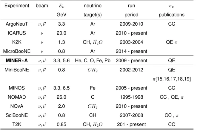
Table 2.1: Experiments focus on cross-sections and oscillation of neutrinos and
the type of channels of interaction focus on.
Experiment beam Eν neutrino run σν
GeV target(s) period publications
ArgoNeuT ν, ~ν 3.3 Ar 2009-2010 CC
ICARUS ν 20.0 Ar 2010 - present
K2K ν 1.3 CH,H2O 2003-2004 QEπ
MicroBooNE ν 0.8 Ar 2014 - present
MINERνA ν, ~ν 3.3, 5.6 He, C, O, Fe, Pb 2009 - present QE
MiniBooNE ν, ~ν 0.8 CH2 2002-2012 QE
π[15,16,17,18,19]
MINOS ν, ~ν 3.3, 6.5 Fe 2005 - present CC
NOMAD ν, ~ν 26.0 C 1995-1998 CC , QE,π
NOvA ν, ~ν 2.0 CH2 2010 - present
SciBooNE ν, ~ν 0.8 CH 2007-2008 CC ,π
T2K ν, ~ν 0.85 CH,H2O 201 - present CC
CHAPTER 2. NEUTRINO EXPERIMENTS 26
Experiments RangeEν Located Source
K2K 1.5 GeV Japan Low neutrino beam
sent from KEK (started 1999)
with a near detector at KEK site
MINOS 3 -12 GeV Fermilab at a distance of 730km
(USA) in the NuMI beamline
high-energy neutrino beam
CNGS 17GeV Gran Sasso 730 km away of
(CERN) Neutrino source at CERN
Table 2.3: Experiments and their detection technology.
Experiment Scope Technology
T2K Reconstruction of Water
neutrino energy spectrum Cherenkov
MINERνA Reconstruction of Calorimetric
neutrino energy spectrum detectors
MicroBooNE Identification and Water
MiniBooNE Reconstruction of Large hydrid
tau neutrinos tracking/emulsion detectors
2.3.1
T2K experiment
T2K (Tokai to Kamioka) is a long-baseline neutrino experiment in Japan that
search for oscillations from muon neutrinos to electron neutrinos, produce by the
intense beam of muon neutrinos with a energy ofhEνi ∼ 0.6GeV J-PARC in the
center of Japan, and directed towards the Super-Kamiokande detector 295km
away.
The near detector (INGRID) is situated 280 meters from the target in the
cen-tre of the neutrino beam, at its objective is to check the direction and intensity
by daily basis of the neutrino beam. The far detector on the other hand, is
lo-cated 100 meters underground in western Japan and is a very large cylinder of
ultra-pure water. By detecting the production of muon and electron neutrinos,
T2K has seen almost 7 times more electron-neutrino events than if there were no
CHAPTER 2. NEUTRINO EXPERIMENTS 27
The physics goals of the experiment is to calculate theνµtoνeoscillation, the
value of mixing angle θ13, precision measurements of oscillation parameters in
νµ disappearance and the search for sterile components in νµ disappearace in
neutral-current events.
(a) (b)
Figure 2.8: Geographical map of the T2K detection the east coast of Japan.
Im-ages from the ofical page of T2K experimenthttp://t2k-experiment.org/.
2.3.2
MiniBoone
Using the beam from Fermilab’s Booster accelerator in the energy region of
Eν = 0.5−1GeV a 800 tons of mineral oil and 1280 PMTs dectector, MiniBoone
was aimed to confirm the excess of electro neutrino events and support the
neu-trino oscillation interpretation of the LSND (Liquid Scintillator Neuneu-trino Detector)
experimentνµνe andν¯µν¯e.
One of the open questions is if there are more neutrinos (”sterile” neutrinos)
that would interact only through gravity. The LSND experiment sets hints in this
direction, puzzling the neutrino community.
As in same case of MINERvA, MiniBooNE detector receive neutrinos
CHAPTER 2. NEUTRINO EXPERIMENTS 28
since the decay length is only 500 meter away. The experiment results finally rule
out a fourth sterile neutrino.
Another currently operating experiment, MicroBooNE, is measuring low en-ergy neutrino cross sections and investigating the low enen-ergy excess events
ob-served by the MiniBooNE experiment. Also, this experiment is testing the future
construction of massive kiloton scale LArTPC detectors for future long-baseline
neutrino physics (DUNE).
(a) MiniBoonE Phototube Support Struc-ture.
(b) MicroBooNE detector at Fermilab
Chapter 3
MINERvA a cross-section neutrino
experiment
As mentioned in the former sections (2.1), (2.2) and (2.3) the neutrino
oscilla-tion experiments need better models of interacoscilla-tion with the detectors. However,
the signal and backgrounds measurements present in the process that are the
poorly measured. MINERvA provide data that considerably improve the models
neutrino-nucleus scattering and thus reduce the systematic uncertainties in the
result from oscillation experiments.
Our experiment (fig. 3.1) is a fine-grained, fully active neutrino detector placed
in the NuMI neutrino beam (3.1.1) with a good high-rate studies of
neutrino-nucleus interactions and good resolution of final states using νµ and νˆµ incident
of 1-20GeV.
In this chapter I will describe the most important components of the MINERvA
detector (3.1), why the experiment includes a scale-down replica of the detector
(3.2.1) and finally the main components of the MINERvA’s Test Beam Experiment
are stated in the last section (3.2).
CHAPTER 3. MINERVA A CROSS-SECTION NEUTRINO EXPERIMENT 30
Figure 3.1: Front view of the MINERvA detector at NuMI Hall at Fermilab.
3.1
”Bringing Neutrinos into Sharp Focus”
MINERvA1is a neutrino experiment dedicated to explore precision neutrino
cross-section measurements in multiple nuclear targets in order to study nuclei and
nuclear effects, as mentioned in [33]:
The experiment provides the opportunity for a broad array of physics
studies, using neutrinos as probes to study nuclear processes and
nu-cleon structure as well as exploring the properties of neutrinos
them-selves. (..) Uncertainties in the cross sections for these processes
contribute to the systematic error of oscillation measurements, so
im-proved measurements of the cross section will contribute directly to
improved precision in the measurement of neutrino oscillation
param-eters.
By receiving around 1020 proton on target, the number of events for CCQE,
Coherent Production of Pions and DIS has improved substantially (we expect
800K events) allowing to study topics that have not been systematically analysed
and/or are plagued by sparse data.
A much complete description of MINERvA physics’ goals can be found on [2],
here we state some of the most relevant:
1This MINERvA web page’s title describe exactly the objective of the experiment https://
CHAPTER 3. MINERVA A CROSS-SECTION NEUTRINO EXPERIMENT 31
• Precision measurement of the quasi-elastic neutrino-nucleus cross-section
including its Eν and q2 dependence and study of the nucleon axial form
factor.
• Determinate the cross-section in the resonance-dominated region for both
neutral-current (NC) and charged-current (CC) interactions.
• Make precision measurements of coherent single-prion production in
car-bon, which is a significant background for next-generation of neutrino
oscil-lation experiments probingνµ→νeoscillation.
• Study of nuclear effects onsin2θ
W measurements, and the NC/CC ratio for
different nuclear targets.
• Improve the measurements of the parton distribution functions with a
ex-pected sample of DIS events.
3.1.1
The NuMI Beam at Fermilab
The NuMI beam (Neutrinos at the Main Injector) is a beam of 120GeV protons
from the Main Injector that collide into a graphite producing secondary pions and
kaons, which are focused with two magnetic horns and directed into a 675m long
decay pipe where most of them decay (eq. 3.1) producing neutrinos and muons.
Muons are absorbed and monitored, through a total of 240 m of rock downstream.
Neutrinos finally reach to the MINERvA and MINOS experiment (fig. 3.2).
µ+→µ++νµ, K+ →µ++νµ
µ−→µ−+ ¯νµ, K− →µ−+ ¯νµ
µ− →e−+νµ+ ¯νe, K+→π0+e++νe
µ+ →e++νe+ ¯νµ, K−→π0+e−+ ¯νe
(3.1)
The NuMI beam provide around 1020protons per target, by a hadron focusing
system it can produce energies of 1-3 GeV (low energy beam), 3-8 GeV or