Trade Deals and/or On-Package Coupons
IGuiomar Mart´ın-Herr´an1,∗, Simon-Pierre Sigu´e2
Abstract
The selection of either a pull or a push price promotion has mainly been investigated in contexts where manufacturers offer deals to consumers at the time of purchase or offer trade deals to retailers. This paper extends this framework to where manufacturers can offer either trade deals or rebate-like promotions to consumers such as on-pack coupons that stimulate the first and second purchases or a combination of the two promotion vehicles. It is demonstrated that the decision to implement either of the three promotion options critically depends, among other factors, on the percentage of first-time buyers who redeem their coupons at the second purchase. Particularly, a necessary condition to simultaneously offer both a trade deal and coupons is to have a positive coupon redemption rate. When possible, manufacturers prefer on-pack coupons over trade deals to take advantage of slippage and to further increase the overall demand via coupon-induced repeat purchase. Manufacturers are more likely to take the lion’s share of channel profits.
Keywords: On-pack coupons, pull price promotions, push price promotions, trade deal
1. Introduction
The issue of whether manufacturers should target their price promotions to their trade partners or final consumers is far from being resolved. Price promotions designed for trade partners such as retailers, also known as push price promotions, generally reduce the regular wholesale prices with the hope that channel partners can find it optimal to fully or partially pass on received price-cuts to consumers and stimulate retail sales, while price promotions targeted at final consumers, known as pull price promotions, directly offer price discounts or other monetary incentives to consumers, with the primary goals of attracting consumers to retail places and stimulating immediate sales. Typically, price promotions are viewed as instruments used by sellers to price discriminate between groups of consumers of varying price sensitivity (Narasimhan, 1984; Varian, 1980; Su et al., 2014). The primary belief underlying this view is that what really matters for consumers is the effective price they pay, regardless of where price cuts may originate.
IWe thank three anonymous reviewers for their helpful comments and suggestions. The first author’s research is partially supported by MICINN under projects ECO2008-01551/ECON and ECO2011-24352, co-financed by FEDER funds.
∗
Departamento de Econom´ıa Aplicada (Matem´aticas), Universidad de Valladolid, Avda. Valle de Esgueva, 6, 47011, Valladolid, Spain. Tel.: +34 983 423330 Fax: +34 983 423299; E-mail: [email protected]
1
IMUVA, Universidad de Valladolid. 2
In this line, traditional economic literature has long considered that the choice between some forms of push and pull price promotions is a simple exercise that exclusively depends on the marketer’s taste as both are expected to provide the same outcomes in terms of retail prices, quantities sold, and channel profits. Cash rebates and trade deals are believed to be two of such price promotions that manufacturers offer indifferently to consumers and retailers in the context of a bilateral monopoly for the same outcomes (Ault et al., 2000). However, this simplistic view of push and pull price promotions as subsidies offered by manufacturers to retailers and consumers is not always theoretically and empirically supported. For instance, Busse et al. (2006) provides with an empirical evidence that the subsidy analogy does not hold in the automobile industry. The effective price consumers paid is lower when a manufacturer offers an identical cash-back to consumers than to retailers. In such an industry where cash rebates alone represent marketing expenses in excess of $3 billion per year (Bruce et al., 2006), a misallocation of promotional budgets can seriously damage manufacturers’ profits and consumer welfare. A few theoretical works have attempted to explain why manufacturers may prefer cash rebates to trade deals. Gerstner and Hess (1991a) find that manufacturers prefer consumer rebates when there is a strong positive association between willingness to pay and redemption costs. Gerstner and Hess (1991b) again claim that manufacturers primarily use cash rebates to motivate retail participation in promotions even when promotions do not discriminate among consumers with different reservation prices. Ault et al. (2000) examine the argument that cash rebates are manufacturers’ first choice because retailers do not fully passed on trade discounts to consumers. They find that even when this argument does not hold, manufacturers could still prefer consumers rebate as trade deals allow retailers to accumulate low-price inventories. Mart´ın-Herr´an et al. (2010) focus on trade promotions that reward retailers for units effectively sold and offer an integrative framework that explains why in some contexts the subsidy analogy may work, and why in some others it may be irrelevant. Mart´ın-Herr´an et al.’s theory supports the view that choosing between trade deals and cash rebates critically depends on the consumer sensitivity to both regular and promotional prices. Particularly, manufacturers are better (worse) off offering trade deals (cash rebates) when consumers are more (less) sensitive to promotions than to regular prices. This theory also claims that the subsidy analogy holds only if consumers react identically to regular and promotional prices.
Departing from cash rebates, Kumar et al. (2004) also investigate the optimal choice between push and pull price promotions in a context where an exogenously sales expansion target is set. The push price promotion in this research is a trade discount offered to retailers, while coupons are used as pull price promotions. It is demonstrated that the manufacturer may choose either trade deals or coupons depending on coupon redemption rates and the equivalence ratio of price reduction to coupon face value.
buys the products. There is therefore a need to further study the trade-offs between push and pull price promotions using promotions with various properties to deepen our understanding of the challenges marketers encounter in the planning of their price promotion programs.
In this paper, we develop a framework where a manufacturer in a bilateral monopoly context has the possibility of offering a trade deal or a rebate-like promotion or a combination of both at the same time. We call rebate-like promotions any promotional activities that require consumers to first purchase the product at the regular price and then benefit from a price discount for the next purchase. We particularly focus on what is known as on-package coupons (Chen et al., 2005; Dhar et al., 1996) where consumers are aware of the pledged discount and it is factored into their decisions to make the first purchase at the regular price. As a consequence, on-package coupons have the potential of directly influencing first and repeat purchases. Our current modeling effort does allow for price discrimination. Due to the slippage phenomenon, consumers who purchase the product in the first period may or may not redeem their coupons in the second period, depending on their price sensitivity, among other factors.
The current research answers the following three questions:
1. What are the conditions under which manufacturers should exclusively offer either trade deals or on-package coupons or a combination of the two promotion types?
2. How does the coupon redemption rate impact on the manufacturers’ profits and, conse-quently, the type of consumer promotions that manufacturers are more likely to imple-ment?
3. How do push and pull price promotions affect the sharing of channel profits?
The rest of the paper is organized as follows: First, we introduce two models: the Benchmark Model (BM) and the Full-Promotion Model (FM). Second, we derive the equilibria, identify the conditions under which the manufacturer may find it optimal to offer push and/or push price promotions, and compare the players’ optimal profits in each scenario. Finally, we conclude by highlighting our contributions to advancing research and practice in this area.
2. The models
Consider a two-member channel of distribution where a manufacturer distributes a single product through an exclusive independent retailer. We build two stylized two-period models to account for various common business situations.
2.1. Benchmark Model
The benchmark model (BM) corresponds to a standard pricing game in which no price incentive is offered (Mart´ın-Herr´an et al., 2010). The manufacturer and retailer each set their regular wholesale price (wi) and regular retail price (pi) at periodi,i∈ {1,2}. We assume that
consumer demand at period iis linear and given by
qi =g−pi,
where g is a positive parameter representing the baseline demand. For simplicity, consumer sensitivity to regular retail price is normalized to 1. Observe that the baseline demand does not change from the first to the second period and that the players keep the same set of decision variables. As a consequence, the first-period game is basically repeated in the second period.
Denote by ΠMi and ΠRi the manufacturer’s and retailer’s profits at period i and assume a constant and positive marginal production cost (c). The two players’ profit functions at period iare given by
ΠMi = (wi−c)qi, ΠRi = (pi−wi)qi, i∈ {1,2}.
Let us assume that the manufacturer is the channel leader and the retailer is the follower. Channel leadership here is decided on an ad hoc basis. However, Jørgensen et al. (2001) endogenously demonstrate that manufacturer leadership is desirable for both manufacturers and retailers, while retailer leadership could be detrimental for channel profits. The following are optimal expressions for the first period in the benchmark model (superscript B):
pB1 = 1
4(c+ 3g), w
B
1 =
1
2(c+g), q
B
1 =
1
4(g−c). (1)
To ensure a positive demand in the first period, condition g > c is needed. From now on, we assume that this condition is always satisfied.
The total manufacturer’s and retailer’s profits are given by
ΠM = ΠM1 +δΠM2 , ΠR= ΠR1 +δΠR2,
channel members and set δ = 1. This assumption is realistic in the context the low interest rates observed in recent years.
The total manufacturer’s and retailer’s optimal profits are given by
ΠM,B= 1 4(c−g)
2, ΠR,B= 1
8(c−g)
2. (2)
The profit function in each period and for each channel member is a strictly concave function with respect to the corresponding decision variable, implying that the necessary conditions for optimality are sufficient too, and that the equilibrium is unique.
Comparing the two channel members’ profits in (2), it is easy to see that the manufacturer earns twice the profit of the retailer. As expected, the Stackelberg manufacturer takes the biggest share of channel profits.
2.2. Full-Promotion Model
The Full-Promotion model (FM) assumes that the manufacturer keeps his first-period regular wholesale price (wB1) unchanged, that he offers both “cents-off” coupons (C) to consumers at the first-period purchase, to be redeemed at the second-period purchase, and a trade deal (d) to the retailer in the first period, and that he controls the second-period wholesale price (w2).
The trade deal in this model should be seen as a discount on the regular wholesale price, which the manufacturer offers to the retailer in the hopes that the latter will, either fully or in part, pass the savings along to consumers in the form of a retailer price promotion. On the other hand, the manufacturer’s coupons targeting the customers directly could have various goals, including attracting new buyers, increasing the consumption of current buyers and retaining new and current customers. Consumers are aware that any coupons unused at the end of the second period of the game are lost.
The retailer endogenously sets a retail price (pi) for each period i, i∈ {1,2}. The demand
functions for each period of the game are given by
q1 = g−pB1 +α(pB1 −p1) +θC,
q2 = g−p2+γ(q1−qB1) +µq1,
wherepB1 is the regular retail price that maximizes the retailer’s profit in the BM,αis a positive parameter representing consumer sensitivity to the promotional price differential. A retail price that is higher during the promotional period than the regular retail price has a negative impact on the first-period demand, while a promotional retail price that is lower than the regular retail price has a positive impact on the first-period demand. We assume that the consumer sensitivity to the regular retail price (here normalized to 1) may be different from the consumer sensitivity to the promotional price differential (α). We assume that 0< α≤1.
We assume that the second-period baseline demand, given by g+γ(q1−qB
1) +µq1, depends
on the source of the first period’s promotional incremental sales (q1−qB1) and on the purchases
from first-period buyers who redeem their coupons (µq1). Observe that if the promotional
activity has no impact on the first-period demand, there is no promotional incremental sales, q1 −qB1 = 0. Normally, however, the first-period demand when coupons are offered should be
higher than the benchmark demand due to the promotional incentive, i.e.,q1−q1B >0. In such
a context, if γ < 0, first-period promotional sales reduce the baseline demand in the second period. This is more likely to occur when current customers buy large quantities to stockpile for future use (purchase acceleration). First-period promotional sales expand the baseline demand in the second period when they are generated by new customers who adopt the product for future use,γ >0 (category expansion). The purchase of larger quantities by current buyers who increase their consumption during the first period and revert to their normal consumption habits in the second period has no significant effect on the second-period sales, γ = 0. On top of these potential traditional post-promotional effects, we model the coupon-induced repeat-purchase effect, which is the demand from the first-period buyers who take advantage of their first-period coupons. Such an effect does not exist when the manufacturer offers instant-rebate or peel-off coupons at the first-period purchase (e.g., Mart´ın-Herr´an et al., 2010). This coupon-induced second-period demand increase is a positive function of both the first-period demand and the redemption rate (µ). We assume that 0 ≤ µ ≤ 1, to account for the slippage phenomenon resulting from the fact that many consumers purchase products to take advantage of future discounts or rebates, but far fewer actually redeem them after their first purchase.
The manufacturer and retailer set their decision variables to maximize their discounted profits during the two periods given by
ΠM = (wB1 −d−c)q1+δ((w2−c)q2−µCq1),
ΠR = (p1−w1B+d)q1+δ(p2−w2)q2.
The decision variables of the two channel members directly impact on the first-period demand. This creates free-riding opportunities. The manufacturer may not offer the desired coupon value, expecting the retailer to compensate with a large pass-through from the trade promotion offer, while the retailer may refrain from doing just that in the hopes that the manufacturer will offer consumers a larger coupon value.
Table 1 summarizes the decision variables, demand functions, and players’ profits for the two models at each period,i,i∈ {1,2}.
Period 1 Period 2 Benchmark Model
Manufacturer’s controls w1 w2
Retailer’s controls p1 p2
Demand functions q1 =g−p1 q2 =g−p2
Manufacturer’s profit ΠM1 = (w1−c)q1 ΠM2 = (w2−c)q2
Retailer’s profit ΠR1 = (p1−w1)q1 ΠR2 = (p2−w2)q2
Full-promotion Model
Manufacturer’s controls C, d w2
Retailer’s controls p1 p2
Demand functions q1 =g−pB1 +α(pB1 −p1) +θC q2=g−p2+γ(q1−qB1) +µq1
Manufacturer’s profit ΠM1 = (w1B−d−c)q1 ΠM2 = (w2−c)q2−µCq1
Retailer’s profit ΠR1 = (p1−wB1 +d)q1 ΠR2 = (p2−w2)q2
We discuss two additional assumptions below.
First, the retailer orders the exact quantity of product that she is able to sell during a given period and therefore holds no inventory. The manufacturer and retailer work together to streamline their supply chain and eradicate inventory costs. Such an integrated system allows the manufacturer to avoid retailer stockpiling during promotions and to reward the retailer for actual sales rather than quantities purchased.
Second, we assume that the production, distribution and processing costs of coupons and trade deals as well as their associated retailer promotions, are zero (e.g., Gerstner and Hess, 1991a&b; and Dhar et al., 1996). As a result, the only direct cost associated to the manu-facturer’s couponing campaign is the transfer payment he makes to the retailer in the second period, as consumers redeem the coupons,µCq1. Redemption costs are believed to be the
criti-cal portion of the cost of couponing (Dhar et al., 1996). Any increase in either the redemption rate, the value of the coupon, or the number of the first-period buyers could potentially harm the manufacturer’s second-period profit.
3. Equilibrium strategies
As stated above, we use the Stackelberg equilibrium concept in the Full-Promotion Model, with the sequence of moves defined as follows. The manufacturer announces his first-period decisions, and the retailer reacts to these announcements, determining her optimal first-period retail price. Then, the manufacturer announces his second-period wholesale price and the retailer reacts to that announcement, determining her optimal second-period retail price. To obtain subgame-perfect equilibria, we solve the game backwards. In other words, we first solve the retailer’s problem in the second period and then substitute the retailer’s optimal decisions into the manufacturer’s second-period problem. Thereafter, the optimal strategies of the second period are incorporated into the players’ total profits. The retailer’s general problem is first solved to determine her first-period retail price, and subsequently, the manufacturer’s general problem is solved to determine the optimal trade deal and coupon value.
respect to his decision variable, while the total profit function may not be concave with respect to his decision variables. As a consequence, an interior equilibrium that maximizes the channel members’ objective functions may be attained only for some specific values of a few model parameters. The following proposition characterizes these possibilities.
Proposition 1. The following two possibilities can arise:
1. If θ−αµ = 0, then the manufacturer’s total profit, ΠM, is a concave function of the manufacturer’s first-period decision variables (C and d). Therefore, the manufacturer’s problem admits an interior solution.
2. If θ−αµ 6= 0, then the manufacturer’s total profit, ΠM, is not a concave function of the manufacturer’s first-period decision variables (C and d). Therefore, the manufacturer’s problem does not admit an interior solution and the solution is attained at the boundary, i.e., at C= 0 or d= 0.
Proof. The first minor of the Hessian matrix of function ΠM with respect to the manufacturer’s first-period decision variables, C and d, always takes negative values for any value of α ∈
(0,1], µ∈[0,1] and γ∈[−1,1]. The determinant of the Hessian matrix is zero for the first case described in the statement of the proposition and negative for the second case. Therefore, the quadratic form associated with the Hessian matrix is negative semidefined and undefined in the first and second cases, respectively. As a result, we can conclude that in the first case, ΠM is a concave function with respect to the manufacturer’s first-period decision variables, C and d, and that an optimal interior solution can be attained; while in the second case, the candidate to be extremum is a saddle point. The maximum is attained at the boundaries.
It is easy to see that Case 1 in Proposition 1 holds when the redemption rate, µ, is zero only when coupons are not effective on the first-period demand (θ= 0). This means that a necessary condition to simultaneously offer both a trade deal and coupons is to have a positive coupon redemption rate, otherwise the manufacturer only offers either a trade deal or coupons if the two promotional activities only impact on the first period-demand. Thus, in addition of the effect of both trade deals and coupons on the first purchase, the manufacturer feels the need to use these two types of promotional activities at the same time to particularly stimulate repeat-purchase, which translates in an increase of the second-period demand.
3.1. Trade deal or Coupons
The following two propositions characterize the equilibrium solutions for the scenarios in which the manufacturer offers either only a trade deal to the retailer or coupons to consumers. The simultaneous offering of the two types of promotion is not a feasible option in this case.
when C= 0 andµ= 0 are as follows:
dC=0 = (g−c)(γ
2α2(8 +γ(4−γ)) + 8α(4 +γ2)−128)
128α(8−γ2α) , (3)
pC1=0 = c+(g−c)(24−α(γ(γ+ 12)−72)−12γ
2α2)
16α(8−γ2α) , (4)
wC2=0 = c+(g−c)(γα(γ(γ−4) + 24)−24γ+ 128)
32(8−γ2α) ,
pC2=0 = c+3(g−c)(γα(γ(γ−4) + 24)−24γ+ 128)
64(8−γ2α) , (5)
and the total manufacturer’s and retailer’s optimal profits are
ΠM,C=0 = (g−c)
2Ω 1
1024α(8−γ2α), (6)
ΠR,C=0 = (g−c)
2Ω 2
4096α(8−γ2α)2, (7)
where
Ω1 = 64 + 16α[88 +γ(γ−20)] +α2[576(1 +γ) +γ2((γ−4)2−144)],
Ω2 = 2(αγ2−8)[3α((γ−2)2−12)−8][8+α((γ−2)2+20)]+α[128+24γ(α−1)+αγ2(γ−4)] 2
.
Proof. See the Appendix.
Remark 1. If coupons are not offered (C= 0) as it is the case in Proposition 2, the first and second-period demand functions are the same as in the trade-promotion model in Mart´ın-Herr´an et al. (2010).
Observe in this scenario that when coupons are not offered (C = 0), the redemption rate is zero (µ= 0). Obviously, without coupons, consumers have nothing to redeem. The analysis of the equilibrium solution in the first scenario (C = 0 and µ = 0) allows for some observations. For any value ofα∈(0,1] andγ∈[−1,1], the following inequalities apply:
p1C=0> c, w2C=0 > c, p2C=0 > c, ΠM,C=0 >0, ΠR,C=0 >0.
However, to ensure that the trade dealdC=0 is positive, the following condition must be satisfied:
α∈(0.618931,1], γ∈(γ,1], (8)
whereγ is the smallest root of the following polynomial equation in the variable γ:
α2(γ−4)γ3−8α(1 +α)γ2−64αγ+ 128(1−α) = 0.
Table 2: Effect ofα on γ.
α γ
0.618931 1
0.62 0.996115
0.75 0.584068
1 0
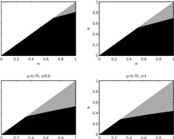
The manufacturer’s decision to exclusively offer a trade deal in this scenario depends on both the consumer sensitivity to the promotional price differential and the incremental promotional sales effect. Condition (8) states that when the consumer sensitivity to a promotional price differential takes relatively high values (α ∈ (0.618931,1]), the nature and the magnitude of the impact of the incremental promotional sales on the second-period demand do matter. If 0.618931≤ α <1, meaning that the consumer sensitivity to the promotional price differential is lower than the consumer sensitivity to regular prices, but higher than the specified threshold, then manufacturers should only offer trade deals to retailers if the expected impact of such pro-motional activities on post-propro-motional sales is positive, i.e., trade deals contribute to expanding the baseline demand for the product. In any case, manufacturers should not offer trade deals to retailers if the consumer sensitivity to the promotional price differential does not reach the threshold of α = 0.618931. Figure 1 displays in gray, the area in the parameter space where the manufacturer finds it optimal to offer the retailer a trade deal.
α
γ
0 0.1 0.2 0.3 0.4 0.5 0.6 0.7 0.8 0.9 1 −1
−0.8 −0.6 −0.4 −0.2 0 0.2 0.4 0.6 0.8 1
Figure 1: Parameter region wheredC=0>0: Gray area
when d= 0 are as follows:
Cd=0 = (g−c)Σ1
64θ[(θ+αµ)(γ+µ)2−16µ], (9)
pd1=0 = c+ (g−c)Σ2
64α[(θ+αµ)(γ+µ)2−16µ], (10)
wd2=0 = c+ (g−c)Σ3
16[(θ+αµ)(γ+µ)2−16µ],
pd2=0 = c+ 3(g−c)Σ3
32[(θ+αµ)(γ+µ)2−16µ], (11)
and the total manufacturer’s and retailer’s optimal profits are
ΠM,d=0 = (g−c)
2Σ 4
512θ[(θ+αµ)(γ+µ)2−16µ], (12)
ΠR,d=0 = (g−c)
2
Σ5
1024α[(θ+αµ)(γ+µ)2−16µ]2
, (13)
where
Σ1 = 16θ(γ(γ−8)−(4 +µ)2)) +µ[128−8α(µ(µ−8) + 4γ(µ−2) + 3γ2−16)
+ α2(γ+µ)2(γ2+γ(µ−4)−4(µ+ 2))],
Σ2 = 16θ(γ(6αµ+µ−4) + 3αµ2−4µ+ (1 + 3α)γ2−8)
+ µ[α2(40 +γ2+γ(µ−4)−4µ)(γ+µ)2−8α(72 + 2γ2+γ(µ−12)−µ(µ+ 12))−64], Σ3 = µ[γ(24−α(µ2+ 8(1−µ))) + 4αµ2−8(1 +α)µ−αγ2(γ+ 2(µ−2))−128]−16θ(γ+µ),
Σ4 = 64θ(θ+αµ)(γ2+γ(µ−4)−4(µ+ 1))−32θµ(γ2+ 4(µ+ 10)−γ(12 +µ))
− µ2(α(γ2+γ(µ−4)−4(µ+ 2))−8)2,
Σ5 = 2[(2θ+µα)(γ2+γ(µ−4)−4(µ+2))−8µ][16θ(γ2(1+α)+γ(µ(2α+1)−4)+µ(αµ−4)−8)
+ µ(α2(γ+µ)2(8+γ2+γ(µ−4)−4µ)−64−8α(8+2γ2+γ(µ−12)−µ(µ+12)))
+ α[αγ2µ(γ+2(µ−2))+4µ(32+4θ+2(1+α)µ−αµ2)+γ(16θ+µ(α(µ2+(1−µ))−24))]2.
Proof. See the Appendix.
Remark 2. The second-period demand in this scenario generalizes that in Mart´ın-Herr´an et al. (2010) to include the coupon redemption rate (µ) and the benchmark retail price (pB1). If the coupon redemption rate is set to zero and α = 1, this scenario becomes identical to the consumer-promotion model in Mart´ın-Herr´an et al. (2010).
andpd=0
1 , w2d=0, pd2=0 are always greater than the unit cost,c, for any value of the parameters in
the defined subsets, except for very low values of µ (for example, µ= 0.1) and extreme values ofγ (i.e.,γ=−1 orγ = 1). In these cases, the following conditions must be added: (0< α <α¯ and 0≤θ≤α) or ( ¯α < α <2 and 0≤θ≤θ(α)).¯
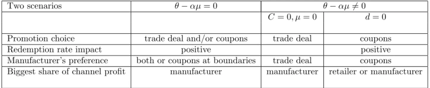
There are additional conditions on parameters α, µ, γ and θ that ensure that the coupon value to consumers, Cd=0, is positive. We refrain from writing these conditions here because they are given by huge expressions3. Numerical simulations allow us to illustrate in Figures 2
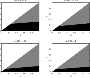
and 3 how some of the model parameters affect the manufacturer’s decision to offer consumer coupons. In Figure 2, let us setµ= 0.25 andγ ∈ {−1,−0.5,0.5,1}and, in Figure 3, γ = 0 and µ∈ {0.25,0.5,0.75,1}.
α
θ
µ=0.25, γ=−1
0 0.2 0.4 0.6 0.8 1 0
0.2 0.4 0.6 0.8 1
α
θ
µ=0.25, γ=−0.5
0 0.2 0.4 0.6 0.8 1 0
0.2 0.4 0.6 0.8 1
α
θ
µ=0.25, γ=0.5
0 0.2 0.4 0.6 0.8 1 0
0.2 0.4 0.6 0.8 1
α
θ
µ=0.25, γ=1
0 0.2 0.4 0.6 0.8 1 0
0.2 0.4 0.6 0.8 1
Figure 2: Parameter region whereCd=0>0: Gray area. µ= 0.25;γ∈ {−1,−0.5,0.5,1}.
Figure 2 shows that the gray area in the parameter space where the manufacturer finds it optimal to offer coupons to consumers expands with the increase of the incremental promotional sales effect on the second-period demand when the redemption rate is hold constant. As ex-pected, the manufacturer is more likely to offer coupons to consumers when they attract new buyers and contribute to expanding the baseline demand in subsequent periods. Figure 3, on the other hand, supports that when the effect of the incremental promotional sales effect is hold constant, the area where the manufacturer offers coupons to consumers contracts with the increase in the redemption rate, which means that coupons are less attractive when they are heavily redeemed. As a result, manufacturers are more likely to offer coupons to consumers when they contribute to expanding the second-period demand by attracting new buyers, but when the coupons are not actually redeemed in large numbers. The explanation behind this
finding is that couponing campaign costs increase as the number of consumers who redeem their coupons in the second period increases, making this promotional activity very costly and less desirable for manufacturers.
α
θ
µ=0.25, γ=0
0 0.2 0.4 0.6 0.8 1 0
0.2 0.4 0.6 0.8 1
α
θ
µ=0.5, γ=0
0 0.2 0.4 0.6 0.8 1 0
0.2 0.4 0.6 0.8 1
α
θ
µ=0.75, γ=0
0 0.2 0.4 0.6 0.8 1 0
0.2 0.4 0.6 0.8 1
α
θ
µ=1, γ=0
0 0.2 0.4 0.6 0.8 1 0
0.2 0.4 0.6 0.8 1
Figure 3: Parameter region whereCd=0>0: Gray area. γ= 0;µ∈ {0.25,0.5,0.75,1}.
Proposition 4. dC=0 and Cd=0 cannot be simultaneously positive.
Proof. The trade deal in the scenarioC = 0, µ= 0,dC=0, is positive if condition (8) is satisfied. It is easy to see that for any value of the parameter space ifµ= 0, the coupon in the scenario d= 0, Cd=0, cannot take positive values.
Proposition 4 deals with Case 2 in Proposition 1 1 and supports the view that, in this particular scenario where, θ−αµ 6= 0, the manufacturer can only provide either of the two promotional activities: C = 0, d > 0 or d = 0, C > 0, but not the two at the same time. As a result, the manufacturer’s choice of any of these promotional activities is done on an ad hoc basis given that their profits cannot be endogenously compared.
Proposition 5. The manufacturer’s profit for the scenariod= 0,ΠM,d=0, is always greater for µ positive than for µ equal to zero.
Proof. The manufacturer’s profit for scenario d = 0 is given by (12). Setting µ = 0 in this expression and by means of numerical simulations, it can be shown that for the range of the parameters for which Cd=0 >0, the result in the proposition holds.
effect on stimulating repeat purchase in the second period cannot be ignored. The coupon-induced repeat-purchase effect contributes to enhancing the appeal of on-pack coupons. As a result, on-pack coupons are more attractive than peel-off coupons or instant rebates (Mart´ın-Herr´an et al., 2010), which only affect the first purchase and do not have any direct effect on subsequent purchases. Further numerical analysis reveal that manufacturers are more likely to earn more profit when coupon redemption (slippage) is lower (higher) than otherwise. As the second-period demand increase via coupon-induced repeat-purchase is achieved by increasing the total cost of the couponing campaign, on-pack coupons should be more beneficial to the manufacturer only when coupons are redeemed by nonregular buyers. Alternatively, if coupons are redeemed by many regular buyers in the second period, the manufacturer’s profitability from the couponing campaign is reduced as these buyers would have anyway purchased the product at the regular price4.
3.2. Trade deal and/or coupons
We turn to the case where the manufacturer can simultaneously offer a trade deal to the retailer and coupons to consumers. The following proposition characterizes the equilibrium solution for this particular case.
Proposition 6. Assumeθ−αµ= 0; then, the Stackelberg equilibrium strategies for the FM are as follows:
d+µC = (g−c)Γ1
128α(8−α(γ+µ)2), (14)
p1 = c+µC+
(g−c)Γ2
16α(8−α(γ+µ)2), (15)
w2 = c+
(g−c)Γ3
32(8−α(γ+µ)2),
p2 = c+
3(g−c)Γ3
64(8−α(γ+µ)2), (16)
and the total manufacturer’s and retailer’s optimal profits are:
ΠM = (g−c)
2
Γ4
1024α(8−α(γ+µ)2), (17)
ΠR = (g−c)
2
Γ5
4096(8−α(γ+µ)2)2
, (18)
4
where
Γ1 = 8α(16+γ2+4γ(µ+2)+µ(3µ+8))−α2(γ+µ)2(γ2+γ(µ−4)−4(µ+2))−128, (19)
Γ2 = α(4(18−µ(3 +µ))−γ(5µ+ 12)−γ2)−12α2(γ +µ)2+ 24,
Γ3 = αγ2(γ+ 2(µ−2)) + 8(1 + 3α)µ−4αµ2+γ(α(24 +µ(µ−8)−24) + 128),
Γ4 = α2[γ4+ 2γ(µ−4)(γ2−4(18 +µ)) +γ2(µ2−16(µ+ 8)) + 16(µ2+ 36(µ+ 1))]
+ 16α(24 + (γ−4)(γ−3µ−16)) + 64,
Γ5 = α[γ(α(24 +µ(µ−8))−24) +αγ3+ 2αγ2(µ−2) + 8µ(3α+ 1)−4αµ2+ 128] 2
+ 2(α(γ+µ)2−8)(α(24 +γ2+γ(µ−4)−4µ) + 8)(3α(γ2+γ(µ−4)−4(2 +µ))−8).
Proof. See the Appendix.
As expression (14) shows, at the equilibrium, the manufacturer has an infinite number of possibilities for his decision variables,C andd, including setting the variables at the boundary, i.e., atC = 0 or d= 0. Any combination of C and dthat satisfies (14) is optimal and leads to the manufacturer’s maximized profit in (18).
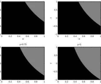
The expression ford+µC given in (14) is positive if the model parameters belong to one of the following two subsets:
α∈(0.375345,0.618931], µ∈(µ,1], γ ∈(γ,1],
α∈(0.618931,1], µ∈[0,1], γ ∈(γ,1],
where boundsµ,γare, respectively, the highest, the lowest, root of the following two polynomials in variablesµ, γ, respectively:
3α2µ3+α(24 + 17α)µ2+α(96 + 25α)µ+α(200 + 11α)−128 = 0,
α2γ4+α2(3µ−4)γ3+ (3α2µ(µ−4)−8α(1 +α))γ2+ (α2µ2(µ−12)−16αµ(α+ 2)−64α)γ +128(1−α)−8αµ(3µ+ 8)−4α2µ2(µ+ 2) = 0.
offer the two promotions when the first-period incremental promotional sales negatively impact on the second-period demand. The rationale is that when consumer sensitivity to promotional price differential is high, the retailer has an incentive to reduce the retail price as a consequence of the trade deal offered by the manufacturer, consumers buy more in the first period, and even with a high redemption rate, the overall revenue increase during the two periods can compensate the related couponing cost supported in the second period.
α
γ
µ=0.25
0 0.2 0.4 0.6 0.8 1 −1
−0.5 0 0.5 1
α
γ
µ=0.5
0 0.2 0.4 0.6 0.8 1 −1
−0.5 0 0.5 1
α
γ
µ=0.75
0 0.2 0.4 0.6 0.8 1 −1
−0.5 0 0.5 1
α
γ
µ=1
0 0.2 0.4 0.6 0.8 1 −1
−0.5 0 0.5 1
Figure 4: Parameter region whered+µC >0: Gray area.θ=αµ, µ∈ {0.25,0.5,0.75,1}.
Remark 3. Let us note that from (14), the following expressions are the manufacturer’s bound-ary promotional strategies:
d = 0, µ6= 0, C = (g−c)Γ1
128αµ(8−α(γ+µ)2), (20)
C = 0, µ= 0, d= (g−c)[α
2γ2(8 + 4γ−γ2) + 8α(4 +γ)2−128]
128α(8−αγ2) , (21)
where Γ1 is given in (19).
This remark highlights the fact that although the manufacturer has the option of offering the two promotions at the same time, nothing prevents him from focusing on only one of them to achieve the maximized profit in (18). In such a context, one of the two boundary solutions in (21) and (22) will be chosen.
On the other hand, Equation (15) establishes that, except forµ= 0, the optimal first-period retail price,p1, is a strictly increasing function of the coupon offered to consumers, C. In other
demonstrated that, under certain conditions, the first-period retail price, p1, in this scenario
remains lower than the benchmark first-period retail price5,pB1. This price can even be lower if C = 0, because of the impact of the manufacturer’s trade deal. Linking the retail price to the value of coupons offered to consumers reduces the effectiveness of both the couponing campaign and the trade deal that the manufacturer simultaneously offer directly to the retailer, especially when consumers are very sensitive to promotional price differentials.
The manufacturer’s and the retailer’s optimal profits are positive, and w2 > c and p2 > c
for any value of α ∈ (0,1], µ ∈ [0,1] and γ ∈ [−1,1]. Also, conditions on the model parame-ters ensuring p1 > c can be derived. The next proposition assesses the impact of the coupon
redemption rate on the manufacturer’s optimal profit.
Proposition 7. The manufacturer’s profit for any optimal strategy given in expression (17) is always higher for µ positive than for µ equal to zero.
Proof. Replaceµ= 0 in (17) and, for the range of the parameters we have fixed, the comparison of this new optimal profit and of the profit in (17) gives the stated result.
Observe that when µ= 0, the manufacturer can only offer a trade deal. Therefore, Propo-sition 7 has two major implications. First, it means that on-pack coupons should be preferred to promotional activities that can impact consumer behavior at the time of the first purchase but that do not induce repeat purchases, like peel-off coupons or instant rebates do. Second, when boundary strategies are considered, as in (20) and (21), the manufacturer is better off adopting the strategy in (20). In other words, in this given area of the parameter space, the manufacturer finds it optimal to offer coupons to consumers instead of a rebate to the retailer, providing that the coupon redemption rate is positive. The rationale is that a trade deal offered only to the retailer acts as a subsidy that the retailer may choose to either partly or fully pass on to consumers to reduce the price paid for their first purchase, while on-pack coupons generate additional sales at the regular price or at an even higher promotional price, and also generate additional coupon-induced repurchases among the first-period buyers.
3.3. Channel profit sharing
We now investigate how the channel profit is allocated between the two channel members. Specifically, we answer the question of who, between the manufacturers and the retailers, earn the most profits in the three scenarios studied above.
Proposition 8. For scenarioC = 0,the manufacturer’s profit, ΠM,C=0, is always greater than the retailer’s profit, ΠR,C=0.
Proof. A comparison of expressions (6) and (7) gives the result.
This scenario offers the possibility to the retailer to fully or partially pocket the trade deal monies received from the manufacturer and increase her unit margin. Proposition 8 claims the manufacturer still earns more profit than the retailer. Remember that the manufacturer’s decision to offer trade deals critically depends on a condition that inversely links two parameters:
consumer sensitivity to the promotional price differential and the incremental promotional sales effect. In such a context, it is also in the retailer’s best interest to partially or fully pass on to consumers the price discount offered by the manufacturer to maximize either the first-period or second-period sales. As a result, the manufacturer’s trade deal offering enhances the profits of the two channel members, but does not dramatically contribute to a shift of channel profits from the manufacturer to the retailer.
Proposition 9. For scenariod= 0, the manufacturer’s profit, ΠM,d=0, can be greater or lesser
than the retailer’s profit, ΠR,d=0, depending on the values of the parameters. Specifically, nu-merical simulations for µ∈ {0.1,0.25,0.5,1}, γ ∈ {−1,−0.5,0,0.5,1}, α∈(0,1] and θ∈[0, α], allow us to conclude that in the following cases:
• µ∈ {0.1,0.25}, γ ∈ {−1,−0.5,0,0.5,1};
• µ= 0.5, γ ∈ {0.5,1};
• µ= 1, γ= 1;
ΠR,d=0 >ΠM,d=0 ⇔ θ(α)¯ < θ < α,
where
• for γ and µ fixed,θ(α)¯ increases asα increases;
• for γ and α fixed, θ(α)¯ increases as µ increases.
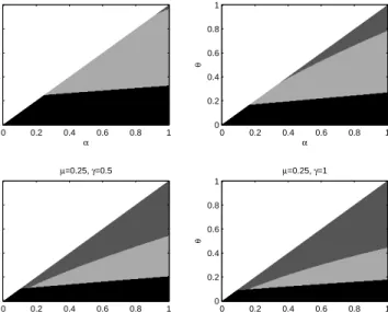
We offer in Figures 5 and 6 an illustration of how µ and γ affect the sharing of channel members’ profits in the parameter space. In Figure 5, µ = 0.25 and γ ∈ {−1,−0.5,0,0.5,1}, while in Figure 6, µ= 0.75 and γ ∈ {−1,−0.5,0,0.5,1}.
There exist four different areas in Figures 5 and 6: the black area whereCd=0is not positive, the light gray area where the manufacturer earns more profit than the retailer, the dark gray area where the retailer earns more profit than the manufacturer, and the white area where the conditionθ≤αis not satisfied. Figure 5 shows that when the redemption rate is relatively small, the area where the retailer earns more profit than the manufacturer grows with the effect of the incremental promotional sales effect. This finding holds regardless of whether the incremental promotional sales effect is positive or negative. Figure 6 demonstrates that when the redemption rate is high enough, the manufacturer is always better off than the retailer.
α
θ
µ=0.25, γ=−1
0 0.2 0.4 0.6 0.8 1 0
0.2 0.4 0.6 0.8 1
α
θ
µ=0.25, γ=−0.5
0 0.2 0.4 0.6 0.8 1 0
0.2 0.4 0.6 0.8 1
α
θ
µ=0.25, γ=0.5
0 0.2 0.4 0.6 0.8 1 0
0.2 0.4 0.6 0.8 1
α
θ
µ=0.25, γ=1
0 0.2 0.4 0.6 0.8 1 0
0.2 0.4 0.6 0.8 1
Figure 5: Parameter region where Cd=0 > 0 and ΠM,d=0 < ΠR,d=0: Dark gray area. µ = 0.25;γ ∈ {−1,−0.5,0.5,1}.
total demand over the two periods, damaging her own overall profitability6. Situations where the retailer deliberately reduces retail prices to support the manufacturer’s couponing campaign are more likely to benefit the two channel members via a substantial increase of the overall two-period demand, especially when consumers are very sensitive to both promotional price differentials and coupons. Therefore, the increase of the retailer’s relative share of profit when the manufacturer offers on-pack coupons should be attributed to the combined promotional efforts of the two channel partners and their second-period effects.
Proposition 10. For the scenario θ−αµ= 0,numerical simulations forµ∈ {0.1,0.25,0.5,1}, γ ∈ {−1,−0.5,0,0.5,1}, α∈(0,1]and θ∈[0, α], allow us to conclude that always ΠR<ΠM.
6
α
θ
µ=0.75, γ=−1
0 0.2 0.4 0.6 0.8 1 0
0.2 0.4 0.6 0.8 1
α
θ
µ=0.75, γ=−0.5
0 0.2 0.4 0.6 0.8 1 0
0.2 0.4 0.6 0.8 1
α
θ
µ=0.75, γ=0.5
0 0.2 0.4 0.6 0.8 1 0
0.2 0.4 0.6 0.8 1
α
θ
µ=0.75, γ=1
0 0.2 0.4 0.6 0.8 1 0
0.2 0.4 0.6 0.8 1
Figure 6: Parameter region where Cd=0 > 0 and ΠM,d=0 > ΠR,d=0: Ligth gray area. µ = 0.75;γ ∈ {−1,−0.5,0.5,1}.
4. Conclusion and discussion
This paper studies a bilateral monopoly channel in which the manufacturer has the possibility of offering a trade deal to the retailer and/or on-pack coupons to consumers. Previous works have studied optimal promotional choices in situations where manufacturers offer trade deals or/and consumer promotional activities that directly and exclusively affect the first purchase. This paper extends this research stream by considering a consumer promotional activity (on-pack coupons) that stimulates both the first and repeat purchases. Table 3 summarizes the main findings of this research.
Table 3: Main findings
Two scenarios θ−αµ= 0 θ−αµ6= 0
C= 0, µ= 0 d= 0
Promotion choice trade deal and/or coupons trade deal coupons
Redemption rate impact positive positive
Manufacturer’s preference both or coupons at boundaries trade deal coupons
Biggest share of channel profit manufacturer manufacturer retailer or manufacturer
The manufacturer has two opposite options: (1) exclusively use either one of the two promo-tional vehicles; or (2) offer various combinations of the two promotions that satisfy a specified condition, including setting the optimal promotions at the boundaries. Whether the manufac-turer only offers coupons to consumers or offers both a trade deal and coupons, the manufacmanufac-turer earns more profits when coupons are redeemed than when they are not redeemed. The man-ufacturer may have no choice but to offer only either a trade deal or coupons; however, when the two types of promotions can be offered simultaneously, the optimal levels of the two pro-motional vehicles are negatively and linearly related. In this particular configuration, however the manufacturer would prefer the exclusive offering of coupons to the exclusive offering of a trade deal. The retailer is more likely to earn more profit than the manufacturer only when the manufacturer solely offers on-pack coupons to consumers and the retailer supports the manu-facturer’s couponing campaign by also discounting the retail price to significantly increase the overall demand over the two periods. In the two other scenarios, the manufacturer still takes the lion’s share of the channel profits, as in the benchmark model where a price promotion is not offered.
Gerstner and Hess (1995) report a similar finding and stress the requirement of complementar-ity between pull and push price promotions when they have to be undertaken together. They support the view that pull price promotions should be combined to push price promotions to improve channel coordination when they are targeted to price-conscious consumers and made less accessible to price-insensitive consumers. Note however that, although our model can price discriminate, in the sense that price-insensitive consumers may not redeem their coupons, price discrimination is not a necessary condition for combining coupons and trade deals. Manufac-turers can still find optimal to offer both trade deals and coupons even if all consumers redeem their coupons at the second period.
Second, the decision to offer either trade deal or on-pack coupons is not always based on the comparison of generated profits. Manufacturers can select either of them on an ad hoc basis using heterogenous factors, overlooked in this work. On the other hand, when manufacturers really do have the option to offer either trade deals or pull price promotions that can stimulate first and second purchases, they make more profits by offering pull price promotions. Mart´ın-Herr´an et al. (2010) instead found that manufacturers are better (worse) off offering trade deals (cash rebates) when consumers are more (less) sensitive to promotions than to regular prices. Trade deals offered only to retailers and cash rebates to consumers act as price subsidies for the first-period purchases. Observe that our current setup goes beyond the impact of a temporary price incentive on the first-period purchases. As a matter of fact, not only do on-pack coupons stimulate first-period purchases at the regular price, on the basis of the promised discount, but they also encourage second purchases, because some coupon holders will redeem them to benefit from the promised discounts. Manufacturers incur promotional costs only when a consumer purchases a second unit. As a result, the overall impact of on-pack coupons on manufacturers’ profits is far higher than any single trade deal program for retailers, where manufacturers incur promotional costs up front for each unit sold. In addition, the slippage phenomenon associated with on-pack coupons enhances their appeal for manufacturers (Yang et al., 2009). Chen et al. (2005) observed that, in some instances, the slippage is large enough to encourage sellers to offer the product for free after a rebate. Their Google search on the key words “free after rebate” generated 1,400,000 results. We performed a similar Google search and found around 14,800,000 results, which indicates a growing interest in promotional vehicles such as on-pack coupons that allow manufacturers to take advantage of slippage.
Finally, based on the comparison of channel members’ total profits, the conventional wisdom stating that manufacturers’ price promotions shift channel profits from the manufacturers to the retailers does not hold when trade deals are offered7. Conversely, when manufacturers exclusively offer on-pack coupons or other price-promotion activities that directly affect both first and repeat purchases, retailers can earn more profits than manufacturers under some identified conditions. As a result, our research adds to the current debate by showing that the on-pack coupon redemption rate as well as the incremental promotional sales effects are key for identifying when retailers are more likely to earn more profits than manufacturers. Particularly, retailers can get the lion’s share of channel profits when the redemption rate is relatively small (large
7
slippage) and the couponing campaign significantly expands the baseline demand. In such a context, both the manufacturer and retailer has mutual incentives to significantly invest in demand expansion. As a result, the retailer supports the manufacturer’s couponing campaign by reducing retail prices. Contrary to the belief that retailers take advantage of manufacturers’ promotional activities to increase their margins, the increase of retailers’ share of channel profits, in such a context, should be attributed to the increase of the overall demand. It is not achieved at the expense of manufacturers’ profits, which also increase. This is consistent with previous papers that support the view that positive long-term effects of promotions benefit both retailers and manufacturers (e.g. Ailawadi, 2001; Sigu´e, 2008).
Our theoretical setup is based on various limiting assumptions, including keeping the bench-mark wholesale price unchanged during the first period of the game, restricting the game to two periods, using a linear demand function, preventing the retailer from stockpiling when the manu-facturer offers a trade deal and disregarding horizontal competition. Some of these assumptions can be relaxed in future research to allow for the examination of more realistic scenarios and the use of other modeling approaches such as the Hotelling model to study horizontal interactions between competing retailers.
Appendix A. Proof of Proposition 2
The game is played in four stages and is solved backwards. We next describe and solve the problem the players are facing at each stage of the game.
Stage 4: At this stage of the game, the retailer chooses the second-period price,p2, in order to
maximize her second-period profits. Therefore, the retailer’s problem can be written as:
max
p2
ΠR2, (A.1)
where
ΠR2 = (p2−w2)q2,
denotes the retailer’s second-period profits and q2 is the second-period demand function given
by
q2 =g−p2+γ(q1−qB1)+µq1 =g−p2+γ(g−p1B+α(pB1−p1)+θC−q1B)+µ(g−pB1+α(pB1−p1)+θC).
(A.2) In the last equality, the expression of the demand function in the first period has been replaced. Recall that bypB1,w1B and q1B we denote the first-period wholesale, the regular retail price and the demand in the benchmark model, which are given in (1).
The solution to problem (A.1) gives us the retailer’s reaction function, that is, p2, as a
function of the wholesale price,w2, of the coupon offered by the manufacturer to consumers,C,
and of the retail price in the first period,p1.
The retailer’s second-period profits is a strictly concave function of her decision variable in this period,p2. From the first-order optimality condition for the problem in (A.1), the following
expression can be derived:
p2 =
1
2(w2+g+ (γ+µ)(g−p
B
Stage 3: At this stage of the game the manufacturer chooses the second-period wholesale price, w2, in order to maximize his second-period profits. Therefore, the problem the manufacturer is
facing can be written as:
max
w2
ΠM2 , (A.4)
where
ΠM2 = (w2−c)q2,
denotes the manufacturer’s second-period profits and q2 is the demand function in this period
defined in (A.2). At this stage of the game, the manufacturer knows the retailer’s pricing reaction function derived in Stage 4, and therefore, incorporates this information when deciding his optimal pricing strategy. Therefore, the reaction function in (A.3) has to be replaced in the manufacturer’s objective function in (A.4).
The solution to this problem gives us the wholesale price,w2, as a function of the retail price
in the first period, p1 and the coupon offered by the manufacturer to consumers, C.
The manufacturer’s second-period profits is a strictly concave function of his decision variable in this period,w2. From the optimality first-order condition for the problem expressed in (A.4)
we get
w2=
1
2(c+g+ (γ+µ)(g−p
B
1 +α(pB1 −p1) +θC)−γq1B). (A.5)
Replacing this expression into the retailer’s reaction function in (A.3) we obtain the second-period retail price as a function of the first-second-period retail price,p1 and the coupon offered by the
manufacturer to consumers, C:
p2=
1
4(c+ 3g+ 3(γ+µ)(g−p
B
1 +α(pB1 −p1) +θC)−γq1B)). (A.6)
The second-period retailer’s and manufacturer’s optimal profits are obtained replacing the expressions (A.5) and (A.6) and they are given by
ΠR2 = 1
256((g−c)(4 +µ−α(γ+µ)) + 4(γ+µ)(αg−αp1+θC))
2, (A.7)
ΠM2 = 1
128((g−c)(4 +µ−α(γ+µ)) + 4(γ+µ)(αg−αp1+θC))
2
− µC
g+1
4(c+ 3g)(α−1)−αp1+θC
, (A.8)
wherepB1,w1B and q1B have been replaced by their values given in (1).
Stage 2: Moving to the first period the retailer chooses the retail price,p1,in order to maximize
her total profits during the two periods:
ΠR= ΠR1 +δΠR2,
Taking into account the second-period retailer’s profits (given by (A.7)) and the optimal retail and transfer price for this period computed in the previous stage ((A.6) and (A.5)), the retailer’s total profits are as follows:
ΠR = (p1−w1B+d)(g−pB1 +α(pB1 −p1) +θC)
+ 1
256((g−c)(4 +µ−α(γ+µ)) + 4(γ+µ)(αg−αp1+θC))
2
.
It can be easily proved that the retailer’ s total profits is a strictly concave function in the retailer’ s first-period decision variable,p1, becauseα(γ+µ)2−16<0 for the range of parameters
we are considering.
Maximizing with respect to the first-period retail price gives the following optimal reaction function, i.e., the first-period retail price,p1, as a function of the deal offered by the manufacturer
to the retailer,d, and the coupon offered by the manufacturer to consumers, C:
p1 =
1
4α(16−α(γ+µ)2)
32(g−pB1 +α(pB1 +wB1)−αd+θC)−4(γ+µ)2α(gα+θC)
− (g−c)α(γ+µ)(4 +µ−α(γ+µ))]. (A.9)
Stage 1: At this stage of the game, the manufacturer chooses the deal,d, offered to the retailer and the coupon,C, offered to consumers in order to maximize his total profits:
ΠM = ΠM1 +δΠM2 ,
where future profits are discounted at rateδ that is assumed to be equal to 1.
Taking into account the second-period manufacturer’s profits (given by (A.8)) and the opti-mal retail and transfer price for this period computed in the previous stages ((A.6) and (A.5)), the manufacturer’s total profits are as follows:
ΠM = (w1B−d−c)(g−pB1 +α(pB1 −p1) +θC)
+ 1
128((g−c)(4 +µ−α(γ+µ)) + 4(γ+µ)(αg−αp1+θC))
2
− µC
g+1
4(c+ 3g)(α−1)−αp1+θC
.
Replacing the retailer’s reaction function given in (A.9), the manufacturer’s total profits to be maximized read:
ΠM = 1
4(16−α(γ+µ)2)2
n
2 [4(αd+θC)(γ+µ) + (g−c)(8 + (α−1)γ+ (α+ 1)µ)]2
− µC(16−α(γ+µ)2)
32(αd+θC) + (g−c)(8−α(γ2+γ(µ−4)−4(µ+ 2)))
+ (w1B−c−d)
g+pB1(α−1)+θC− 1
4(16−α(γ+µ)2)
4[(αc+θC)(8−α(γ+µ)2)−8α(d−c)]
+ (g−c)[8−3α2(γ+µ)2+α(40−(γ+µ)(4 +µ))] .
First, in Proposition 2 we focus on the boundary solution C= 0. Maximizing function ΠM
with respect to the deal offered by the manufacturer to the retailer,d, taking into account that C= 0, and hence, µ= 0, the optimal expression dC=0 given in (3) is obtained.
Replacing this expression in the retailer’s reaction function given in (A.9), we obtain the optimal retail price for the first period.
The final expressions of the optimal pricing strategies and the manufacturer’s and retailer’s profits given in the statement of Proposition 2 can be obtained oncepB
1, wB1 and q1B have been
substituted by their values in (1).
Appendix B. Proof of Proposition 3
The derivation of the equilibrium strategies in Proposition 3 follows the same steps as in Proposition 2. Both proofs share Stages 4, 3 and 2. At Stage 1 now we focus on the boundary solutiond= 0. Maximizing function ΠM with respect to the coupon offered by the manufacturer
to consumers, C, taking into account that d = 0, the optimal expression Cd=0 given in (9) is obtained. Once this expression is known, the final expressions of the optimal pricing strategies and the manufacturer’s and retailer’s profits given in the statement of Proposition 3 can be easily derived.
Appendix C. Necessary and sufficient conditions for Cd=0 >0 Conjecture 1. For µ∈(0,1]and γ ∈[−1,1],
Cd=0 >0 ⇔ α < α≤1 and θ(α)< θ≤α. (C.1)
• Forγ fixed,α increases asµ increases.
• Forµ fixed, α decreases as γ increases.
• Forγ andµ fixed, θ(α) increases as α increases.
• Forµ and α fixed, θ(α) decreases as γ increases.
• Forγ andα fixed, θ(α) increases asµ increases.
Appendix D. Proof of Proposition 6
The derivation of the equilibrium strategies in Proposition 6 follows the same steps as in Proposition 2. Both proofs share Stages 4, 3 and 2. At Stage 1 now assumeθ−αµ= 0 and from Proposition 1, ΠM is a concave function of the manufacturer’s first-period decision variables (C
and d) and, therefore, the manufacturer’s problem admits an interior solution.
Maximizing function ΠM with respect to the deal offered by the manufacturer to the retailer, d, and with respect to the coupon offered by the manufacturer to consumers,C, the expression in (14) that establishes the relationship between the two manufacturer’s decision variables at the optimal levels is obtained.
References
[1] Ailawadi, Kusum L. (2001), “The Retail Power-Performance Conundrum: What Have We Learned?,”Journal of Retailing, 77, 299–318.
[2] Ault, Richard., T. Randolph Beard, David N. Laband and Richard P. Saba (2000), “Re-bates, Inventories, and Intertemporal Price Discrimination,”Economic Inquiry, 38(4), 570-578.
[3] Bruce, Norris, Preyas S. Deai and Richard Staelin (2006), “Enabling the Willing: Consumer Rebates for Durable Goods,”Marketing Science, 25(4), 350–366.
[4] Busse, Meghan, Jorge Silva-Risso and Florian Zettelmeyer (2006), “$1,000 Cash Back: The Pass-Through of Auto Manufacturer Promotions,”The American Economic Review, 96(4), 1253–1270.
[5] Chen, Yuxin, Sridhar Moorthy and Z. John Zhang (2005), “Price Discrimination After the Purchase: Rebates as State-Dependent Discounts,”Management Science, 51(7), 1131–1140.
[6] Demirag, Ozgun Caliskan, Pinar Keskinocak and Julie Swann (2011), “Customer Rebates and Retailer Incentives in the Presence of Competition and Price Discrimination,”European Journal of Operational Research, 215(1), 268-280.
[7] Dhar, Sanjay K., Donald G. Morrison and Jagmohan S. Raju (1996), “The Effect of Package Coupons on Brand Choice: An Epilogue on Profits,”Marketing Science, 14(2), 192–203.
[8] Farris, Paul W. and Kusum L. Ailawadi (1992), “Retail Power: Monster or Mouse?,” Journal of Retailing, 68(4), 351–369.
[9] Gerstner, Eitan and James D. Hess (1991a), “Who Benefits from Large Rebates: Manufac-turer, Retailer, or Consumer?,”Economic Letters, 36, 5-8.
[10] Gerstner, Eitan and James D. Hess (1991b), “A Theory of Channel Price Promotions,”The American Economic Review, 81(4), 872–886.
[11] Gerstner, Eitan and James D. Hess (1995), “Pull Promotions and Channel Coordination,” Marketing Science, 14(1), 43–60.
[12] Gilpatric, Scott M. (2009), “Slippage in Rebate Programs and Present-Biased Preferences,” Marketing Science, 28, 229–238.
[13] Jørgensen, Steffen, Simon P. Sigu´e and Georges Zaccour (2001), “Stackelberg Leadership in a Marketing Channel,”International Game Theory Review, 3(1), 1–14.
[14] Kumar, V. Vibhas Madan and Srini S. Srinivasan (2004), “Price Discounts or Coupon Promotions: Does it Matter?,”Journal of Business Research, 57, 933-941.
[16] Mart´ın-Herr´an, Guiomar, Simon P. Sigu´e and Georges Zaccour (2010), “The Dilemma of Pull and Push-Price Promotions,”Journal of Retailing, 86(1), 51–68.
[17] Mart´ın-Herr´an, Guiomar and Simon P. Sigu´e (2011), “Prices, Promotions, and Channel Profitability: Was the Conventional Wisdom Mistaken?,”European Journal of Operational Research, 211(2), 415-425.
[18] Messinger, Paul R. and Chakravarthi Narasimhan (1995), “Has Power Shifted in the Gro-cery Channel?,”Marketing Science, 14(2), 189–223.
[19] Narasimhan, Chakravarthi (1984), “A Price Discrimination Theory of Coupons,”Marketing Science, 3(2), 128–147.
[20] Nijs, Vincent R., Marnik G. Dekimpe, Jan-Benedict E.M. Steenkamp and Dominique M. Hanssens (2001), “The Category-Demand Effects of Price Promotions,”Marketing Science, 20(1), 1–22.
[21] Sigu´e, Simon P. (2008), “Consumer and Retailer Promotions: Who Is Better Off?,”Journal of Retailing, 84(4), 449–460.
[22] Srinivasan, Shuba, Keon Pauwls, Dominique M. Hanssens and Marnik G. Dekimpe (2004), “Do Promotions Benefit Manufacturers, Retailers, or Both?” Management Science, 50(5), 617–629.
[23] Su, Meng, Xiaona Zheng, Luping Sun. (2014), “Coupon Trading and Its Impacts on Con-sumer Purchase and Firm Profits, ”Journal of Retailing, 90(1), 40-61.
[24] Varian, Hal R. (1980), “A Model of Sales,”American Economic Review, 70(4), 651–659.