The TCLUST Approach to Robust
Cluster Analysis
∗
L.A. Garc´ıa-Escudero, A. Gordaliza,
C. Matr´
an and A. Mayo-Iscar
Departamento de Estad´ıstica e Investigaci´on Operativa
Universidad de Valladolid. Valladolid, Spain
†Abstract
A new method for performing robust clustering is proposed. The
method is designed with the aim of fitting clusters with different
scat-ters and weights. A proportionαof contaminating data points is also
allowed. Restrictions on the ratio between the maximum and the
min-imum eigenvalues of the groups scatter matrices are introduced. These
restrictions make the problem to be well-defined guaranteeing the
ex-istence and the consistency of the sample estimators to the population
parameters.
∗Research partially supported by Ministerio de Ciencia y Tecnolog´ıa and FEDER grant
MTM2005-08519- C02-01 and by Consejer´ıa de Educaci´on y Cultura de la Junta de Castilla
y Le´on grant PAPIJCL VA102A06.
†Departamento de Estad´ıstica e Investigaci´on Operativa. Facultad de Ciencias.
The method covers a wide range of clustering approaches, which
arise depending on the strength of the chosen restrictions. Our
pro-posal includes an algorithm for approximately solving the sample
problem which takes advantage of the Dykstra’s algorithm.
Key words: Robustness; Cluster Analysis; trimming; asymptotics;
trimmed k-means; EM-algorithm; fast-MCD algorithm; Dykstra’s
al-gorithm.
Abbreviated title: Robust clustering based on trimming.
1
Introduction
Many statistical practitioners view the Cluster Analysis as a collection of
mostly heuristic techniques for partitioning multivariate data. This view
re-lies on the fact that most of the cluster techniques are notexplicitly based on a probabilistic model. This could “...lead the naive investigator into
believ-ing that he or she did not make any assumption at all, and that the results
therefore are ‘objective’...” (Flury 1997, page 123). However, that
objective-ness is far from the reality as long as most of the times the cluster’s results
are strongly affected by the chosen method and its performance is somehow
very dependent on the assumed underlying probabilistic model for which the
method is implicitly aimed to. For instance, when using k-means, we must keep in mind that this method is designed for clustering spherical groups of
roughly equal sizes and, thus, the method is not reliable when the groups
understand clustering methods and decide which method should be applied
in a particular case it is interesting to determine appropriate models and
develop methods specially tailored for these models.
That determination of appropriate models for clustering is even more
important in the presence of noisy data or outliers. Without specifying a
model, it is not clear what we understand by an observation following an
“anomalous” behavior. For instance, it is not clear when a set of very
scat-tered observations may be seen indeed as an extra proper group or merely
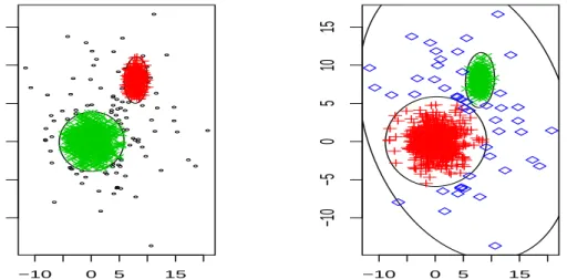
as a background noise to be deleted (see Figure 1). Additionally, it is not
−10 0 5 15
−10
−5
0
5
10
15
(a)
−10 0 5 15
−10
−5
0
5
10
15
(b)
Figure1: (a) Two groups with 10%of the observation discarded (trimmed points
are the small circles). (b) Three groups partition with no observations discarded.
obvious wether a small group of tightly joined outliers should be considered
as a proper group instead of a contamination phenomenon. Finally, notice
that the precise detection of the outliers is very important due to the serious
Garc´ıa-Escudero and Gordaliza 1999 and Hennig 2004) and also due to the appealing
interest they could have by themselves after explaining why they depart from
the general behavior.
Bock (2002) mentions in a recent Cluster Analysis review paper two
model-based approaches which provide a “theoretical well-based clustering
criterion” in presence of outliers:
(i) Mixture modelling: This first approach is based on considering mixture fittings. Some examples are the MCLUST and the EMMIX software.
MCLUST (Fraley and Raftery 1998) allows the addition of a mixture
component accounting for the “noise” (usually modelled by a uniform
distribution in a convex set containing all the observations). McLachlan
and Peel (2000)’s EMMIX tries to fit the noise resorting to mixtures of
t distributions.
(ii) Trimming approach: The second approach assumes a known fractionα
of outliers to be trimmed off and, later, the non-trimmed observations
or “regular” data are split intok groups. Examples of this approach are the trimmed k-means (Cuesta-Albertos et al. 1997) and some recent proposals by Gallegos (2001, 2002) and Gallegos and Ritter (2005).
Notice that a “crisp” 0-1 approach is usually adopted in the second
ap-proach while the mixture apap-proach generally returns some groups’ ownership
probabilities. However, the main difference between these two approaches
the outliers are completely discarded (being trimmed-off) in the trimming
approach. The methodology presented in this paper is included within the
second, “trimming”, approach and all the comparisons will be made within
this category of methods. The so-called “spurious-outlier” model commented
below will serve as a common model for this approach.
The ability of trimming the least reliable observations has played
histor-ically a very important role as a way of providing robustness to many
statis-tical procedures. Nevertheless, trimming in Cluster Analysis is not
straight-forward because no privileged directions there exist for searching outlying
values and, most of the times, we even need to remove observations which
fall between the groups (“bridge” data points). The first attempts of
trim-ming in clustering appeared in Cuesta-Albertos et al. (1997). There, a
modification of the k-means method (the most widely used non-hierarchical clustering method) is presented. The way to perform the trimming is called
“impartial” as it is the sample itself which tells us the observations to be
discarded. Moreover, Garc´ıa-Escudero and Gordaliza (1999) showed that
the impartial trimming provides better results in terms of robustness than
the consideration of different penalty functions in the k-means method (e.g.,
k-medoids).
The use of trimmed k-means involves a considerable drawback in how it implicitly assumes the same spherical covariance matrix for the groups (as
classicalk-means does). This justifies the recent extension for that method in Gallegos and Ritter (2005) through the trimmed determinant criterion. This
but it allows for a general expression of the common covariance matrix non
necessarily spherical. There, it also appears a statistical clustering model
with outliers called thespurious-outlier model extending the usual statistical clustering setup (Mardia et al. 1979) to consider the presence of a proportion
α of noise. The likelihood function for the data set {x1, ..., xn} is
·Yk
j=1
Y
i∈Rj
f(xi;µj,Σ)
¸· Y
i /∈R
gψi(xi)
¸
(1.1)
with R = ∪k
j=1Rj and #R = [n(1−α)]. The parameter k denotes the to-tal number of groups, Rj contains the indexes of the “regular” observations assigned to group j and f(·;µ,Σ) stands for the p.d.f. of the p-variate nor-mal distribution with mean µand covariance matrix Σ while gψi’s are some p.d.f.’s in Rp. If Σ = σ2 ·I is chosen in (1.1) then we would be perform-ing the trimmed k-means method. Gallegos and Ritter (2005) showed that the maximization of (1.1) reduces to the consideration of the regular part of
the observations under just some reasonable assumptions for the gψi’s when-ever the “non-regular” observations may be seen as merely “noise”. In spite
of that, the maximization of this classification likelihood is a
computation-ally hard problem because of its combinatorial nature. Therefore, they also
propose an algorithm in the spirit (both algorithms coincide when k = 1) of the fast-MCD in Rousseeuw and van Driessen (1999) for approximately
maximizing (1.1).
The assumption for the equality of the groups’ covariance matrices could
be very restrictive in many contexts. Therefore, the next natural extension
ex-pression (1.1). Unfortunately, this heterogeneous robust clustering problem
is notably harder. It is easy to see the unboundedness of the proposed
ob-jective function, as each data point gives rise to a singularity on the edge
of the parametric space. Moreover, a straight adaptation of the fast-MCD
algorithm is not longer adequate. The inadequacy of a na¨ıve adaptation
follows from the disturbing presence of different groups’ “scales” (we define
the “scale” parameter for a covariance matrix Σj as |Σj|1/p) which makes
complex the global ordering of the observations around their closest centers
through Mahalanobis distances (see, Garc´ıa-Escudero and Gordaliza 2006)
when performing the so-called “concentration” steps. This is the reason why
unrestricted algorithms frequently find clusters containing a few data points
either very close together or almost lying in a lower dimensional space
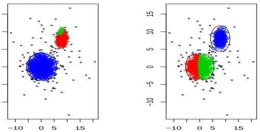
(Fig-ure 2,a) and the application of some kind of restriction would allow us to
obtain (perhaps) more interesting or informative partitions (Figure 2,b).
As a way of posing constraints to the heterogeneous robust clustering
problem, Gallegos (2001, 2002) proposes normalizing the covariances to have
unit determinant when computing the Mahalanobis distances in the
“concen-tration” steps. This serves to avoid the harmful effect of the different scales
and even so benefiting from the rationale behind the fast-MCD algorithm.
Gallegos’s procedure works nicely when the groups have similar scales, but
it does not work so well when very different groups’ scales are involved.
Nor-malizing the covariances to have unit determinant can be very restrictive
and, surely, such strong restrictions are not always needed. Moreover, it
−10 0 5 15
−10
−5
0
5
10
15
(a)
−10 0 5 15
−10
−5
0
5
10
15
(b)
Figure 2: An unrestricted solution for the same data set in Figure 1 appears in
(a) when k = 3 and α = .1. Compare with a restricted partition, also when
k = 3 and α = .1, in (b). A description of the applied clustering methods will be given in Section 3.
statement instead of (artificially) appearing in the algorithm.
Having these things in mind, constraints for the heterogeneous robust
clustering problem will be incorporated in this paper through an
eigenvalues-ratio restriction. A constant cwill control the strength of the posed restric-tion entailing a wide range of clustering problem depending on its value.
Finally, it can be shown that the heterogeneous robust clustering
prob-lem is even notably harder under the presence of different weights for the
underlying groups. Hence, the introduction of some weight terms πj’s in (1.1) will also be considered for handling different groups’ weights. In fact, it
can be easily shown that do not include the weights in the objective function
Since we assume that every point in the sample spaceRp will be assigned
to some group (or it is part of the sample space to be discarded), we will be
able to define a population counterpart serving as a probabilistic benchmark.
Existence results for both, the sample and the population problems, will be
given in this Section 2. Moreover, consistency of the sample maximizers to
the population ones under mild assumptions is proven. The proofs of these
results make clearer the importance of the eigenvalues restrictions in order
to guarantee these existence and consistency results.
In Section 3, we propose a feasible algorithm (TCLUST) for
approxi-mately solving the sample version of the problem. The algorithm may be
seen as a Classification EM-algorithm (Celeux and Govaert 1992) where a
kind of “concentration” step is also applied. The eigenvalues-ratio
restric-tions will be imposed by solving a constrained least squares problem. Dykstra
(1983)’s algorithm may be applied for addressing that problem.
Finally, Section 4 shows a simulation study showing the gain provided by
the proposed method with respect to other “trimming” proposals.
2
Robust Clustering with Eigenvalues-Ratio
Restrictions
a function f by P f(·) =R f(x)dP(x).
2.1
Mathematical formulation
We start by modifying the “spurious-outlier” model considered in Gallegos
and Ritter (2005). First, as mentioned before, we consider different scatter
matrices Σi’s as in Gallegos (2001, 2002). Moreover, we assume the presence
of some underlying weights πj’s with
Pk
j=1πj = 1 associated to the distri-butions generating the set of “regular” observations. This leads us to the
maximization of
·Yk
j=1
Y
i∈Rj
πjf(xi;µj,Σj)
¸· Y
i /∈R
gψi(xi)
¸
, (2.1)
with R =∪k
j=1Rj and #R =n−[nα]. Additionally, the restrictions on the eigenvalues of the Σj’s matrices will be later introduced in order to avoid
sin-gularities. As in Gallegos and Ritter (2005), if the gψ’s satisfy the condition
arg max
R
max
µj,Σj
k
Y
j=1
Y
i∈Rj
πjf(xi;µj,Σj)⊆arg max
R
Y
i /∈∪k
j=1Rj max
ψi
gψi(xi)
where R stands for the set of all partitions of the indexes {1, ..., n} onto k
groups of regular observations, R, and a group containing the non-regular ones, with #R = n−[nα], then we can avoid the non-regular contribution to the previous maximization problem. This condition easily holds under
just some reasonable assumptions for the gψi’s whenever the “non-regular” observations are seen as merely “noise”. For instance, the examples for gψi’s shown in the Gallegos and Gallegos and Ritter’ papers can be trivially also
considered here. We refer the interested reader to these papers for more
Additionally, for an easier statement of our problem, we will use some
assignment functions zj’s telling us which classeverypointxinRp is assigned to (not only the sample observations xi’s are classified). We follow a 0-1 “crisp” approach where x is
assigned to the class j if zj(x) = 1,
or
it is being trimmed off if z0(x) = 1.
With these functions, assuming that the gψi’s may be omitted, we can raise again the problem in (2.1) to the maximization of
n
Y
i=1
·Yk
j=1
πzj(xi)
j f(xi;µj,Σj)zj(xi)
¸
,
with zj being 0-1 functions defined in the whole sample space verifying
Pk
j=0zj(xi) = 1 and
Pn
i=1z0(xi) = [nα]. This statement of the problem, taking logarithms, leads us to the following general one:
Robust Clustering problem: Given a probability measure P, we search for the maximization of:
P
" k X
j=1
zj(·)
¡
logπj + logf(·;µj,Σj)
¢#
, (2.2)
made in terms of the assignment functions:
zj :Rp 7→ {0,1}, such that k
X
j=0
zj = 1 and P z0(·) = α,
and the parameters θ = (π1, ..., πk, µ1, ..., µk,Σ1, ...,Σk) corre-sponding to weights πj ∈ [0,1] with
Pk
µj ∈ Rp and symmetric positively definite p ×p-matrices Σj,
j = 1, ..., k.
If Pn stands for the empirical measure, Pn = 1/n
Pn
i=1δxi, we just need to replace P by Pn in the previous problem in order to recover the origi-nal sample problem (notice that, perhaps, Pnz0(·) = α can not be exactly achieved but this familiar fact will not be very important in our reasonings).
Let us finally introduce our restrictions on the eigenvalues of the
covari-ance matrices. This type of restriction may be seen as an extension of those
introduced by Hathaway (1985) for one-dimensional data. It allows to avoid
the singularities introduced by the possibility of very different Σj’s by
con-trolling the ratio between the maximum and the minimum eigenvalue of these
matrices:
(ER) Eigenvalues-Ratio restrictions: We fix a constantc≥1 such that
Mn/mn≤c for
Mn= max
j=1,...,k l=1max,...,pλl(Σj) and mn= minj=1,...,k l=1min,...,pλl(Σj)
where λl(Σj) are the eigenvalues of the matrices Σj, j = 1, ..., k and l = 1, ..., p.
Notice that, the strongest possible restriction follows from setting c= 1. In this particular case, the proposed method may be viewed as a trimmed k -means method with weights. However, the main advantage of this approach
relies on the fact that parameter c allows us to achieve certain (controlled) freedom in how we want to handle the different scatter of the groups. Figure
1 and 2 in Section 1 show the results of the application of the proposed
methodology (by using the TCLUST algorithm described in Section 3) to a
data set made up of three gaussian 2-dimensional clusters where the most
scattered one accounts for 10% of the data. The result when k = 2, α =.1 and c= 5 appears in Figure 1,(a). The result there is not very dependent on
c as long as the two (main) groups are not too different in their eigenvalues once the most scattered group has been trimmed off. The values k = 3 and
α = 0 were considered in Figure 1,(b), with a large value forc(c= 50) which allows for the presence of the more scattered group. The values k = 3 and
α =.1 were applied in Figure 2. A rather largec(unrestricted) was chosen in Figure 2,(a) while a small c= 1 (restricted) was considered in Figure 2,(b).
Once our problem was stated, we must exclude in the subsequent
analy-sis those probability distributions obviously unappropriate for this approach.
This leads us to assume on the underlying distribution P the following mild condition which trivially holds if it is a continuous distribution or if it is the
empirical measure Pn corresponding to a sample from an absolutely contin-uous distribution (for n large enough):
The distribution P is not concentrated on k points after removing a
To conclude this section, we will notably simplify our problem through an
adequate reformulation. This will lead to express the assignment functions
zj’s only in terms of θ. This new statement will be of capital importance for deriving later an algorithm to solve the sample counterpart of the problem.
In order to state this result, some additional notation will be needed:
Given θ∈Θc, we consider some discriminant functions defined as
Dj(x;θ) = πjf(x;µj,Σj)
and
D(x;θ) = max{D1(x;θ), ..., Dk(x;θ)}
(notice that these functions appear when applying Bayes’ rules in
Discrimi-nant Analysis). These functions will serve to determine which are the most
“outlying” observations. For a fixed choice of θ, the smaller D(x;θ) for a given x is, the more outlyingx will be supposed.
Using the previous definitions, for a given θ and a probability measure
P, we define
G(·;θ, P) :u∈R7→P
·
I[0,u](D(·;θ))
¸
(2.4)
and
R(θ, P) :=G−1(α;θ, P) = inf
u {G(u;θ, P)≥α}
(notice that if X is a random variable with distribution given by P then
R(θ, P) is the α-quantile of the random variableD(X;θ)).
Lemma 1 For a probability measure P, using the discriminant functions Dj(x;θ), the Robust Clustering problem can be simplified to the maximization
only on terms of θ of
θ7→L(θ, P) := P
" k X
j=1
zj(·;θ) logDj(·, θ)
#
, (2.5)
where the assignment functions are obtained from θ as
zj(x;θ) = I{x:{D(x;θ) =Dj(x;θ)} ∩ {Dj(x;θ)≥R(θ, P)}}
and
z0(x;θ) = 1− k
X
j=1
zj(x;θ).
In other words, we assign x to the class j with the largest discriminant function value Dj(x;θ) orx is trimmed off when all theDj(x;θ)’s (and con-sequently D(x;θ)) are smaller than R(θ, P). To be more precise, a rule for breaking ties in the discriminant function values is also needed. For
in-stance, the lexicographical ordering could be applied. The proof of Lemma
1 is straightforward and it will be omitted.
2.2
Existence
Our analysis begins by proving the existence of solutions for the proposed
problem:
Consider a sequence{θn}∞n=1 ={(π1n, ..., πnk, µn1, ..., µnk,Σn1, ...,Σnk)}∞n=1such that
lim
(the boundedness from below for (2.6) can be easily obtained just considering
π1 = 1, µ1 = 0, Σ1 = I, and setting the other weights as 0 with arbitrary choices of means and variances).
Since [0,1]k is a compact set, we can extract a subsequence from {θ
n}∞n
(that will be denoted like the original one) such that
πn
j →πj ∈[0,1] for 1≤j ≤k, (2.7) and also satisfying for some g ∈ {0,1, ..., k} (a relabelling could be needed) that
µnj →µj ∈Rp for 0≤j ≤g and min
j>g kµ
n
jk → ∞. (2.8) With respect to the scatter matrices, if the restriction ER is assumed, we
can also consider a further subsequence verifying one (and only one) of these
possibilities:
Σnj →Σj for 1≤j ≤k, (2.9)
Mn= max
j=1,...,k l=1max,...,pλl(Σj)→ ∞, (2.10)
or
mn= min
j=1,...,k l=1min,...,pλl(Σj)→0. (2.11)
The next lemma will show the convergence of the covariance matrices by
showing that only the convergence (2.9) is possible:
Lemma 2 If ER holds and if P satisfies (2.3), then the convergences (2.10) or (2.11) for the covariance matrices are not possible. Therefore, we can find subsequences of Σn
Proof: We will see that (2.10) or (2.11) would imply limn→∞L(θn, P) =−∞. Let λn
l,j := λl(Σnj) be the eigenvalues , j = 1, ..., k and l = 1, ..., p, of the group covariance matrices andvn
l,j their associated eigenvectors withkvnl,jk= 1. We see that
L(θn, P) = P
" k X
j=1
zj(·;θn)
¡
logπnj − p
2log 2π− 1 2
p
X
l=1
logλnl,j
−1 2
p
X
l=1
(λn
l,j)−1(· −µnj)0vl,jn(vnl,j)0(· −µnj)
¢#
≤ P
" k X
j=1
zj(·;θn)
¡
logπn
j −
p
2log 2π−
p
2logmn− 1 2M
−1
n k · −µnjk2
¢#
(2.12)
If we assume that (2.10) holds, i.e. Mn → ∞, then mn → ∞ by ER. Thus, we would have thatL(θn, P)→ −∞and this leads us to a contradiction with (2.6).
Now assume that (2.11) holds. We will need a technical result which
guarantees that if P satisfies (2.3), then there exists a constant h such that
P
" k X
j=1
zj(·;θn)k · −µnjk2
#
≥h >0. (2.13)
The proof of this result is based on an existence result for trimmed k-means (Cuesta-Albertos et al. 1997) and it is left to the Appendix.
Since logπn
j ≤0, the fact that P[z1(·) +...+zk(·)] = 1−α implies
L(θn, P)≤(1−α)
¡
−p
2log 2π−
p
2logmn
¢ −1 2M −1 n P " k X j=1
zj(·;θn)k · −µnjk2
#
.
Therefore, ER and (2.13) give
L(θn, P)≤(1−α)
¡
− p
2log 2π−
p
2logmn
¢
− 1 2(cmn)
But this upper-bound in (2.14) tends to −∞ as mn →0. ¤
By applying the previous lemma, let us consider a subsequence verifying
(2.7), (2.8) and (2.9). We will see that whenever the classes in the
opti-mal partition have strictly positive probability masses we can guarantee the
convergence of the centers µn
j. These result will be of key importance to
understand the role played by the weights πj’s in this approach.
Lemma 3 When ER and (2.3) hold, if every πj in (2.7) verifies πj > 0,
j = 1, ..., k, then g = k in (2.8) (i.e., the centers µn
j are not allowed to
arbitrarily increase in norm).
Proof: If g = 0, we can take a ball with center 0 and radius big enough
B(0, R) such that P[B(0, R)]> α. We can thus easily see that
P
" k X
j=1
zj(·;θn)k · −µnjk2
#
→ ∞,
so thatL(θn, P)→ −∞from (2.12). Notice that condition ER has also been applied.
When g >0, we prove first that
P
"
k
X
j=g+1
zj(·;θn)
#
→0. (2.15)
This arises from the dominated convergence theorem taking into account that
the sequence is obviously bounded by 1−α, and the fact that
{x:zj(x;θn) = 1} ⊆ {x: max
j=g+1,...,kDj(x;θn)≥D1(x;θn)} (2.16)
We can now use (2.15) in order to get:
lim
n→∞supL(θn, P)
≤ lim
n→∞P
" g X
j=1
zj(·;θn)
¡
logπn
j −
p
2log 2π− 1 2log|Σ
n
j| −
1 2(· −µ
n
j)0(Σnj)−1(· −µnj)
¢#
= P
" g X
j=1
zj(·; ˜θ)
¡
logπj −
p
2log 2π− 1
2log|Σj| − 1
2(· −µj)
0Σ−1
j (· −µj)
¢#
,
where x 7→ zj(x; ˜θ) are the assignment functions which would be derived when working with g (instead of k) populations and ˜θ being equal to a limit of the subsequence {θ˜n}∞n=1 ={(π1n, ..., πng, µn1, ..., µng,Σn1, ...,Σng)}∞n=1.
As Pgj=1πj < 1, the proof ends up by showing that we can change the weights π1, ..., πk by
πj∗ = Pgπj
j=1πj
for 1≤i≤g and π∗g+1 =...=πk∗ = 0, (2.17) (and properly modifying the assignment functions zj’s). This change pro-duces a strict decrease in the objective function, leading to a contradiction
with the optimality stated in (2.6). Thus, we conclude g =k. ¤
Proposition 1 (Existence) If (2.3) holds for the probability measure P, then there exists some θ ∈ Θc such that the maximum of (2.6) under the
restriction ER is achieved.
Proof: The existence of such as θ follows easily from Lemmas 2 and 3: (i) If πn
j →πj >0 for 1≤j ≤k, then the choice of θ is obvious. (ii) Now assume that πn
j → πj > 0 with πj > 0 for j ≤ g and πj = 0 for
g < j ≤k. We define the weightsπj as
πj = lim
n→∞π
n
Analogously, takeµj = limn→∞µnj and Σj = limn→∞Σnj forj ≤g. The otherµj’s and Σj’s may be arbitrarily chosen (but with the eigenvalues of the Σj’s verifying the restriction possed by ER). ¤
Although we admit weights πj = 0, this is not a drawback when taking logπj because in this casezj(·;θ)≡0 and then set{x:zj(x;θ) = 1}is empty. Notice that the presence of groups with zero weight does actually happen in
practice. For instance, when k = 2, c = 1, α = 0 and P is the N(0,1) distribution in the real line, we can see that θ = (π1, π2, µ1, µ2, σ21, σ12) = (1,0,0, µ2,1,1) is the optimal solution for every µ2 ∈R.
Recall that the objective function for the trimmed k-means method al-ways improves when increasing k (see, Lemma 9 in the Appendix). The analysis of the optimal values for these objective functions leads to an useful
criterion for deriving appropriate choices of the parameters k andα (Garc´ıa-Escudero et al. 2003). Here, the possible existence of groups with πj = 0 would imply that the value of the objective function does not necessarily
improve when increasing k. However, this property could be even more in-teresting in order to develop better techniques for choosing k and α.
2.3
Consistency
Given{xn}∞n=1 an i.i.d. random sample from an underlying (unknown) prob-ability distribution P, let {θn}∞n=1 ={(π1n, ..., πkn, µn1, ..., µnk,Σn1, ...,Σnk)}∞n=1 ⊂ Θc denote the sequence of sample estimators obtained by solving the
Section 2.2 shows that such sequence does always exist, for large enoughn, whenever P is an absolutely continuous distribution verifying (2.3). Notice that although similar notation to that applied in previous section will be
used, here the index n will indicate the dependence on a random sample of size n fromP.
2.3.1 Boundedness of the sample estimators
We will see first that there exists a compact set K ⊂ Θc such that θn ∈ K for n sufficiently large with probability 1.
Lemma 4 If P is an absolutely continuous distribution (thus verifying con-dition (2.3)) then the elements of the matricesΣn
j are uniformly bounded with
probability 1.
Proof: We see first that there exists a constant M0 such that
L(θn, Pn)≥M0 >−∞ P-a.e. for n≥n0. (2.18)
Due to the tightness of Pn, we can find a sequence of radii {rn} uniformly bounded by a constant r such that Pn(B(0, rn))≥ 1−α. Thus we trivially have
L(θn, Pn)≥
Z
B(0,rn)
µ
− p
2log 2π− 1 2kxk
2
¶
dPn(x) with {I{B(0, s)}(·)(−p
2 log 2π− 1
2k · k2) : s ≤ r} being a Glivenko-Cantelli class and so (2.18) follows.
In order to see the boundedness of the elements of the covariance matrices,
the minimum eigenvalue mn does not tend to 0. We start again from (2.12) with P = Pn, but the analogous of (2.13) follows from another trimmed k -means result shown in Appendix entailing the existence of a constanth0 such
that
Pn
" k X
j=1
zj(·;θn)k · −µnjk2
#
≥h0 >0 (2.19)
whenever P satisfies (2.3). The proof follows similar steps to that of Lemma 2. IfMn → ∞ormn→0 then we would have that L(θn, Pn)→ −∞,P-a.e., and (2.18) does not hold. ¤
Lemma 5 If P is an absolutely continuous distribution, then we can choose empirical centersµn
j,j = 1, ..., k, such that their norms are uniformly bounded
with probability 1.
Proof: Assume on the contrary that for every sequence of optimal centers we can find a further subsequence (denoted as the original one) and satisfying
(2.8) for someg < k. We will see that this is not possible by considering two possible alternatives:
(i) Let us assume, first, that there exist strictly positive limit points
corre-sponding to the associated sequences of empirical weights {πn
j}∞n=1 for
every j = 1, ..., k. I.e., there exist a subsequence such that
πn
j →πj0 >0 for j = 1, ..., k.
(2.16), together with the P-a.e. boundedness of the sample covariance matrices, easily implies that
Pn
" k X
j=g+1
zj(·;θn)
#
→0.
As we did in the proof of Lemma 3, we can define a new sequence {θen} obtained from{θn}such that the weights ˜πnj forj = 1, ..., gare obtained after distributing the initial weights of the groups whose probability
mass tend to 0 as in (2.17) and setting ˜πn
j = 0 for j = g + 1, ..., k. Let us also consider ˜µn
j = µnj for j = 1, ..., g and some arbitrary but uniformly bounded centers ˜µn
j for j =g+ 1, ..., k. We would see that lim
n→∞L(
e
θn, Pn)< lim
n→∞L(θn, Pn),
eventually contradicting the optimal character of the {θn} sequence.
(ii) Let now assume that there exits a j such that the only limit points of the sequence {πn
j}∞n=1 are zeroes value (i.e., πjn →0 forj =g + 1, ..., k for g < k), then it is easy to see again, due to the P-a.e. boundedness of the covariance matrices, that we could replace the original centers for
some uniformly bounded ones without decreasing L(·, Pn) for n large enough with probability 1. ¤
2.3.2 Consistency result
Let us start by stating the Glivenko-Cantelli property for two classes of
Lemma 6 Given a compact set K, the classes of functions:
H1 :=
©
I[u,∞)
¡
D(·;θ)¢:θ ∈K, u≥0ª (2.20)
and
H2 :=
©
I[u,∞)
¡
D(·;θ)¢ k
X
j=1
z∗
j(·;θ) logDj(·;θ) :θ∈K, u≥0
ª
(2.21)
are Glivenko-Cantelli classes, where z∗
j(x;θ) = I{x:D(x;θ) =Dj(x;θ)}(all
the observations in Rp are assigned to some class without trimming by ussing
the z∗
j’s).
Proof: The sets {x : D(x;θ) ≥ r} are the union of k ellipsoids in Rp. The functions logDj(x;θ) = logπj + logf(x;µj,Σj) are polynomials of degree 2 and the sets {x : z∗
j(x;θ) = 1} can be obtained through the intersection of subgraphs of polynomials of degree 2.
The Glivenko-Cantelli class properties are so easily obtained by using the
methodology in section 2.6 of van der Vaar and Wellner (1996). ¤
A technical result on R(θ;P) = G−1(α;θ, P) with G(·;θ, P) defined in (2.4) is also needed:
Lemma 7 Let P be an absolutely continuous distribution with an strictly positive density function. Then, for every compact subset K, we have that
sup
θ∈K
|R(θ;Pn)−R(θ;P)| →0, P-a.e. . (2.22)
Proof: For every δ >0, we can find an ε >0 such that
Otherwise, for a given δ, we could find a sequence {θn}∞n=1 ⊂K satisfying
G(R(θn, P) +δ, P, θn)−G(R(θn, P)−δ, P, θn)<1/n.
Thus, as the θn are included in the compact set K and R(θn, P) ≤ M, we could choose a further convergent subsequence (denoted as the original one)
such that θn→θ0 ∈K and R(θn, P)→r0 for a value r0 ≥0 (we apply that
R(θ, P) are uniformly bounded forθ ∈K).
Notice that the conditions assumed onP imply that u7→ G(u, P, θ) is a continuous and strictly increasing function. Therefore, we would have that
G(r0 +δ, P, θ0) = G(r0 − δ, P, θ0), and this would contradict the strictly increasing character of G(·, P, θ).
Now, if (2.22) did not hold, we could choose another sequence{θn}∞n=1 in
K such that
|R(θn, Pn)−R(θn, P)|> δ
for someδ >0. Therefore, by applying (2.23), we would see thatG(R(θn, Pn), P, θn) is smaller than α−ε/2 or greater thanα+ε/2 infinitely often.
On the other hand, the Glivenko-Cantelli class property for H1 in (2.20)
entails
sup
θ∈K,u≥0
|G(u, Pn, θ)−G(u, P, θ)| →0, P-a.e., and we obtain
|G(R(θn, Pn), P, θn)−G(R(θn, Pn), Pn, θn)| →0, P-a.e..
We can state now the main result in this section which it is the consistency
result:
Proposition 2 (Consistency) Assume that P has an strictly positive den-sity function and thatθ0 is the unique maximum of (2.2) under the restriction
ER. If θn ∈ Θc denotes a sample version estimator based on the empirical
measure Pn, then θn→θ0 almost surely.
Proof: We have proved the existence of a compact set K such that θn ∈ K for n ≥n0 with probability 1.
Notice that our objective function in the empirical case can be rewritten
as:
L(θ, Pn) =
Z
{x:D(x,θ)≥R(θ;Pn)}
·Xk
j=1
z∗
j(x;θ) logDj(x;θ)
¸
dPn(x).
Define new objective functions as
e
L(θ, Pn) =
Z
{x:D(x,θ)≥R(θ;P)} ·Xk
j=1
z∗j(x;θ) logDj(x;θ)
¸
dPn(x),
(where R(θ, P) is fixed only depending on P and not depending on Pn). We can see that
sup
θ∈K
|L(θ;Pn)−Le(θ;Pn)|=oP(1),
by using Lemma 7 and the fact that the integrand can be bounded from
above and below from some constants uniformly for θ in the compact set K. Finally, we can resort to the Glivenko-Cantelli property for the class of
functionsH2 in (2.21), and apply Theorem 3.2.3 in van der Vaar and Wellner
Remark 1 Notice that a uniqueness condition is needed in order to
estab-lish the consistency result. Unfortunately, this property does not always
hold. For instance, think of a symmetric mixture P in the real line with two well-separated modes, a high trimming level and k = 1. The uniqueness property was already needed for establishing the same consistency result for
the trimmed k-means and, even in this simpler case, the statement of gen-eral uniqueness results was difficult (see Remark 4.1 in Garc´ıa-Escudero et
al. 1999). However, as in the trimmed k-means problem, we believe that it is quite rare to find a distribution where the uniqueness fails, when dealing
with “reasonable” data for clustering and when parameters k and α have been properly chosen.
3
The TCLUST algorithm
The empirical problem presented in Section 2.1 has obviously a very high
computational complexity. An exact algorithm seems to be not feasible even
for moderate sample sizes. Thus the existence of an adequate algorithm
for approximately solving the sample problem can be as important as the
procedure itself. With this in mind, we propose the TCLUST algorithm, an
EM-principle based algorithm, intended to search for approximate solutions.
The EM algorithm is the usual method of obtaining a solution to the mixture
likelihood problem (Dempster et al. 1977). Here, as we follow a “crisp”
approach where each point is uniquely assigned to one cluster, a classification
observations are allowed, the rationale behind the fast-MCD (Rousseeuw
and van Driessen 1999) and behind the trimmedk-means algorithm (Garc´ıa-Escudero et al 2003) will also underly. The restriction on the eigenvalues will
be incorporated through Dykstra (1983)’s algorithm.
The TCLUST algorithm may be described as follows:
1. Randomly select starting values for the centers m0
j’s, the covariance
matrices S0
j’s and the weights of the groups p0j’s forj = 1, ..., k. 2. From theθl= (pl
1, ..., plk, ml1, ..., mlk, S1l, ..., Skl) returned by the previous iteration:
2.1. Obtain di = D(xi, θl) for the observations {x1, ..., xn} and keep the set H having the [n(1−α)] observations with largest di’s. 2.2. Split H into H = {H1, ..., Hk} with Hj = {xi ∈ H :Dj(xi, θl) =
D(xi, θl)}.
2.3. Obtain the number of data pointsnj inHj and their sample mean and sample covariance matrix,mj and Sj,j = 1, ..., k.
2.4. Consider the singular-value decomposition ofSj =Uj0DjUj where
Uj is an orthogonal matrix andDj = diag(Λj) is a diagonal matrix (with diagonal elements given by the vector Λj). If the full vector
of eigenvalues Λ = (Λ1, ...,Λk) does not satisfy the eigenvalues-ratio restriction, obtain through Dykstra’s algorithm a new vector
˜
the inverse of the elements of the vector Λ. Notice that the ER
restriction for Λ correspond exactly to the same ER restriction
applied to Λ−1.
2.5. Updateθl+1 using: • pl+1
j ←- nj/[n(1−α)]
• ml+1
j ←- mj
• Sjl+1 ←- U0
jDejUj and Dej = diag(˜Λj)−1
3. Perform F iterations of the process described in step 2 (moderate val-ues for F are usually enough) and compute the evaluation function
L(θF;P
n).
4. Draw random starting values (i.e., start from step 1) several times, keep
the solutions leading to minimal values of L(θF, P
n) and fully iterate
them to choose the best one.
The computed (E-step) ‘a posteriori’ probabilities,Dj(xi, θl) = pjf(xi;mj, Sj), are converted to a discrete classification where we leave unassigned the
pro-portion α of observations which are the hardest to classify. It is easy to see that this lead us to an optimal assignment.
We later obtain a new θl+1 by maximizing (M-step) the conditional ex-pectation once all untrimmed observation have been assigned to the groups.
Proposition 3 guarantees that the presented algorithm can be applied for
performing this maximization. Notice that the obtention of the optimal
eigenvalues and eigenvectors. For every choice of eigenvalues, the best
eigen-vectors choice simply follows from the unitary eigeneigen-vectors of the sample
covariance matrix of the observations assigned to each group. This
decom-position is somehow similar to that considered in Gallegos’ proposal, where
the “shapes” and the “scales” are separately handled.
If we see D(xi, θl) as an inverse outlyingness measure for the observation
xi with respect to a choice of θl, then step 2 may be seen as some kind of “concentration” steps. Garc´ıa-Escudero and Gordaliza (2006) analyzes
some other attempts for extending the “concentration” step principle to the
heterogeneous robust clustering setup.
Recall that the random initialization scheme (step 1) and the final
refine-ment (step 4) were very important in the fast-MCD algorithm. For
initializ-ing the procedure in the step 1, we have seen that simply randomly choosinitializ-ing
k sample data points for the centers, k identity matrices for the covariances and the same weights for the groups (equal to 1/k) provide reasonably start-ing values in most of the cases.
With respect to the eigenvalues-ratio restriction, we would need Λ =
(Λ1, ...,Λk) with Λj = (λ1,j, ..., λp,j) belonging to the cone C, where
C ={(Λ1, ...,Λk)∈Rp×k :λu,v−c·λr,s≤0 for all (u, v)6= (r, s)}. (3.1)
If Λ ∈ C, we need to replace Λ/ −1 by ˜Λ ∈ C with minimalkΛ˜ −Λ−1k2. Dyk-stra’s algorithm serves to approximately solve that constrained least squares
problem when C is the intersection of the several closed convex cones by
be seen as the intersection of the cones
Ch ={(Λ1, ...,Λk)∈Rp×k :λu,v−c·λr,s≤0}, h= (u, v, r, s),
and the projections onto the cones Ch are very fast to obtain. Thus a fixed
number of individual projections may be done retaining the best attained
solution after these iterations and satisfying the restrictions. Alternatively,
quadratic programming based solutions (see, e.g., Goldfarb and Idnani 1983)
to that constrained minimization may be explored.
Next result serves to formalize the appropriateness of the TCLUST
algo-rithm:
Proposition 3 If the setsHj ={xi :zj(xi) = 1}, j = 1, ..., k, are kept fixed,
the maximum of (2.2) for P =Pn can be obtained through the following steps:
(i) Fixed µj and Σj, the best choice of πj is πj = nj/[n(1− α)] where
nj = #Hj.
(ii) Fixed Σj and the optimal values for πj given in (i), the best choice for
µj is the sample mean mj of the observations in Hj.
(iii) Fixed the eigenvalues for the matrix Σj and the optimum values given
in (i) and (ii) for πj andµj, the best choice for the set of unitary
eigen-vectors are the unitary eigeneigen-vectors of the sample covariance matrix Sj
of the observations in Hj.
Proof: Once the zj(xi) for i= 1, ..., n and j = 0, ..., k are known values, the expression (2.2) can be written as
k
X
j=1
·
njlogπj +
X
xi∈Hj
logf(xi;µj,Σj)
¸
, (3.2)
and the assertions (i) and (ii) trivially hold.
Considering these optimal values for πj and µj, together with the cyclic property of the trace, the maximization of (3.2) simplifies to the minimization
of
k
X
j=1
·
log|Σj|+ trace(Σ−j1Sj)
¸
.
The matrices Sj and Σj can be decomposed into Sj = Uj0DjUj and Σj =
V0
jEjVj, where Dj = diag(Λj) and Ej = diag(Ξj) are diagonal matrices Λj = (λ1,j, ..., λp,j) and Ξj = (ξ1,j, ..., ξp,j), and Uj and Vj are orthogonal matrices. So, as log|Σj| = log|Ej| and the eigenvalues Ej were fixed, the previous minimization problem can be further simplified to that of
k
X
j=1
trace(Σ−1
j Sj) =
k
X
j=1
trace(E−1
j (UjVj0)0Dj(UjVj0)).
(the cyclic property of the trace is again applied). Denote Tj = UjVj0, and, rewrite
trace(Ej−1Tj0DjTj) =
X u X v λu,j ξv,j
·t2u v,j , (3.3)
where tu v,j denotes the element (u, v) of the matrix Tj. As long as Tj is an orthogonal matrix, we have that Put2
u v,j = 1 and
P
vt2u v,j = 1. Therefore,
the minimization of (3.3) may be seen as a linear programming problem like
minX u,v
cu,v ·xu,v subject to
X
u
xu,v = 1,
X
v
with known coefficientscu,v (notice thatλu,j/ξu,j are fixed coefficients because
λu,jdepends on the data set at hand and theξu,jare supposed known values in (iii)). Although fractional solutions are possible, these solutions will never be
basic feasible ones due to the particular statement of the linear programming
problem (see, e.g., Papadimitriou and Steiglitz 1982, pg. 249). Consequently,
the optimal solution corresponds to a “real matching” where the optimal t2 u,v
are 0 or 1. Thus, Tj is a permutation matrix product of the orthogonal matrices Uj and Vj0. It is quite easy to see that the columns of the matrices
Uj and Vj must provide the same set of unitary eigenvectors and, thus, the assertion (iii) is proven.
By applying (i),(ii) and (iii), we finally need to search for a vector Ξ =
(Ξ1, ...,Ξk) minimizing k
X
j=1
p
X
i=1
µ
logξi,j+
λi,j
ξi,j
¶
= k
X
j=1
p
X
i=1
¡
−log ˜λi,j+λi,j·˜λi,j
¢
, with ˜λi,j = 1/ξi,j. (3.4)
As (3.4) is a convex function on the ˜λi,j and its unrestricted minimum is attained when ˜λi,j = λ−i,j1, the minimization of (3.4) under the eigenvalues-ratio restriction possed by (3.1) leads us to the optimal choice of ˜Λ with
minimal kΛ˜ −Λ−1k2 and ˜Λ∈ C. ¤
Remark 2 Alternatively, other methods can be defined by imposing
restric-tions on the ratio between the determinant of the groups’ covariances instead
of controlling the eigenvalues. Gallegos (2001, 2002)’s proposal scales the
co-variance matrices to have determinant ratio equal to 1 in the algorithm.
normalization as the only reliable “distance” for clustering multivariate data.
The algorithm proposed here can be easily adapted for handling restrictions
of this type. In this case, the cone would be
C0 ={(σ1, ..., σk)∈Rk:σu−c·σv ≤0 for all u6=v},
and the factorization in step 2.4 of the algorithm isSj =σj·Uj with|Uj|= 1 and σj = |Sj|1/p. If c = 1 in C0, we would have an analogous of Gallegos’s proposal with groups’ weights.
Moreover, other procedures which have been used for avoiding
patholog-ical solutions in the heterogeneous robust clustering problem are based on
adding different types of parameterizations for the covariance matrices (see,
e.g., Scott and Symons 1971 or Banfield and Raftery 1993). Although that
possibility has not been considered here, we believe that similar ideas (based
on relaxing those parameterizations) could be interesting.
4
A simulation study
A simulation study has been carried out to compare the performance of
the proposed robust clustering method with respect to other trimming
ap-proaches in the literature. Several data sets of size n = 2000 have been generated. Each data set consists of two simulated p-dimensional normally distributed clusters with centersµ1 = (8,0,0, ...,0)0andµ2 = (0,8, ...,0)0 and covariance matrices
The constants a, b and c serve to control the true differences between the eigenvalues of the groups’ covariance matrices leading us to the following
cases:
(M1) (a, b, c) = (1,1,1): Spherical equally scattered groups.
(M2) (a, b, c) = (5,1,5): Not spherical but the same covariance matri-ces for the groups.
(M3) (a, b, c) = (5,5,1): Different covariance matrices but the same scale (equal determinant).
(M4) (a, b, c) = (1,20,5): Groups with different scales.
(M5) (a, b, c) = (1,45,30): Groups with different scales and a severe overlap.
We consider 1800 “regular” data points and, in order to take into account
the groups’ weights, a proportion ρ of them are generated from the first normal distribution and a proportion (1 − ρ) from the second. We also generate uniformly distributed data points in a parallelogram defined by
the coordinatewise ranges of the regular data points. Using an
acceptance-rejection algorithm, only points having squared Mahalanobis distances from
µ1 and µ2 (using Σ1 and Σ2) greater thanχ2p,.975 are finally considered until reaching an amount of 200 clear outliers.
The following approaches searching fork= 2 groups and with a trimming proportion α=.1 are tried:
(GR) Gallegos and Ritter’s method (specially aimed to the case M2).
(G) Gallegos’s proposal (specially aimed to the case M3).
(TCLUST) The presented algorithm with an eigenvalues-ratio restric-tion c= 50.
The same number of random initializations and “concentration” steps are
considered for all methods.
Table 1 shows the average proportion of misclassified observations for
B = 1000 independent random samples of size 2000 when p = 2 and 6 and the groups’ weights are ρ= 1/2 and 1/3.
Notice that all the methods work nicely under the underlying model they
are specially aimed to. However, the proposed eigenvalues-ratio restriction
method is the only method which is able to cope with the mixtures with very
different scales (mixtures M4 and M5) and it seems to be less affected in the
unequal groups’ size case. Figure 3 shows the result of these four analyzed
procedures applied to the same data set generated by the simulation scheme
M5 when p = 2 and ρ = 1/3. The proposed method seems to be the only one able to distinguish between the least and the most scattered group even
in this rather overlapped case.
APPENDIX
The following lemma was applied in the proofs of Lemmas 3 and 4. Its
−10 0 10 20 30
−10
0
10
20
TkM
−10 0 10 20 30
−10
0
10
20
GR
−10 0 10 20 30
−10
0
10
20
G
−10 0 10 20 30
−10
0
10
20
TCLUST
Figure3: Clustering results whenk= 2andα=.1for a simulated data following
the M5 scheme in the text with p= 2 and ρ= 1/3: Trimmed k-means (TkM);
Gallegos and Ritter (GR); Gallegos (G) and the presented algorithm (TCLUST)
Lemma 8 (i) IfP satisfies condition (2.3) then there exists a constanth >0
such that inequality (2.13) holds.
(ii) If P is an absolutely continuous distribution satisfying condition (2.3), then there exists a constant h0 > 0 such that (2.19) holds with probability 1
for n large enough.
Proof: (i) For a given probability measureP, the trimmedk-means problem is stated by the search of gpointsµ1, ..., µg inRp and a Borel setB minimizing:
min
B:P(B)≥1−α µ1min,...,µk
1
P(B)
Z
B inf
1≤j≤kkx−µjkdP(x). (4.1) This paper contains an existence result which guarantees that problem
(4.1) always has a solution, so it attains a minimum value that it can be
denoted here by Vα,k. Now, for every choice of θ, we can see that:
P
" k X
j=1
zj(·;θ)k · −µjk2
#
≥P
" k X
j=1
zj(·;θ) inf
1≤j≤kk · −µjk 2
#
≥(1−α)Vα,k,
because ∪k
j=1{x : zj(x;θ) = 1} is a Borel set having probability greater or equal than 1 −α. Finally, we trivially see that h := Vα,k > 0 whenever condition (2.3) holds for P.
(ii) The associated sample problem follows from (4.1) when considering
P =Pn. Let us denote by Vα,kn the minimum value attained by the objective function of this sample problem. Theorem 3.6 in Cuesta-Albertos et al.
(1997) entails the consistency Vn
α,k →Vα,k,P-a.e., and Vα,k >0 if P satisfies the condition (2.3). ¤
Lemma 9 If Vα,k denotes the minimum value attained by (4.1) when k
Proof: The proof of this result corresponds to Lemma 2.2. in Cuesta-Albertos et al. (1997). ¤
References
[1] Banfield, J.D. and Raftery, A.E. (1993), “Model-based Gaussian and
non-Gaussian clustering,” Biometrics, 49, 803-821.
[2] Bock, H.-H. (2002), “Clustering methods: from classical models to new
approaches,” Statistics in Transition, 5, 725-758.
[3] Celeux, G. and Govaert, A. (1992), “Classification EM algorithm for
clustering and two stochastic versions”,Comput. Statit. Data Anal., 13, 315-332
[4] Cuesta-Albertos, J.A., Gordaliza, A. and Matr´an, C. (1997), “Trimmed
k-means: An attempt to robustify quantizers,” Ann. Statist., 25, 553-576.
[5] Dempster, A., Laird, N., and Rubin, D. (1977), “Maximum likelihood
from incomplete data via the EM algorithm,” J. Roy. Statist. Soc. B, 39, 1-38.
[6] Dykstra, R.L. (1983), “An algorithm for restricted least squares
regres-sion,” J. Amer. Statist. Assoc., 78, 837-842.
[8] Fraley, C. and Raftery, A.E. (1998), “How many clusters? Which
clus-tering method? Answers via model-based cluster analysis,” The Com-puter J., 41, 578-588.
[9] Gallegos, M.T. (2001), “Robust clustering under general normal
assump-tions”, preprint avaliable at http://www.fmi.uni-passau.de/forschung/ mip-berichte/MIP-0103.html.
[10] Gallegos, M.T. (2002), “Maximum likelihood clustering with outliers”,
in Classification, Clustering and Data Analysis: Recent advances and applications, K. Jajuga, A. Sokolowski, and H.H. Bock eds., 247-255, Springer-Verlag.
[11] Gallegos, M.T. and Ritter, G. (2005), “A robust method for cluster
analysis,” Ann. Statist., 33, 347-380.
[12] Garc´ıa-Escudero, L.A. and Gordaliza, A. (1999), “Robustness properties
of k-means and trimmed k-means,” J. Amer. Statist. Assoc., 94, 956-969.
[13] Garc´ıa-Escudero, L.A. and Gordaliza, A. (2007), “The
impor-tance of the scales in heterogeneous robust clustering,” Comput. Statit. Data Anal., 51, 4403-4412.
[14] Garc´ıa-Escudero, L.A., Gordaliza, A. and Matr´an, C. (1999), “A
[15] Garc´ıa-Escudero, L.A., Gordaliza, A. and Matr´an, C. (2003), “Trimming
tools in exploratory data analysis,” J. Comput. Graph. Statist.,12, 434-449.
[16] Goldfarb, D. and Idnani, A. (1983). A numerically stable dual method
for solving strictly convex quadratic programs. Mathematical Program-ming 27, 1-33.
[17] Hathaway, R.J. (1985), “A constrained formulation of maximum
like-lihood estimation for normal mixture distributions,” Ann. Statist, 13, 795-800.
[18] Hennig (2004), “Breakdown points for ML estimators of location-scale
mixtures,” Ann. Statist., 32, 1313-1340.
[19] Mardia, K.V., Kent, J.T. and Bibby, J.M. (1979),Multivariate Analysis,
Academic Press, London, New York, Toronto, Sydney, San Francisco.
[20] Maronna, R. and Jacovkis, P.M. (1974), “Multivariate clustering
proce-dures with variable metrics,” Biometrics, 30, 499-505.
[21] McLachlan, G. and Peel, D. (2000), Finite Mixture Models,John Wiley Sons, Ltd., New York.
[23] Rousseeuw, P.J. and Van Driessen, K. (1999), “A Fast Algorithm for
the Minimum Covariance Determinant Estimator,” Technometrics, 41, 212-223.
[24] Scott, A.J. and Symons, M.J. (1971), “Clustering based on likelihood
ratio criteria,” Biometrics, 27, 387-397.
Weights Dimensions Mixtures TkM GR G TCLUST
ρ= 1/2 p= 2 M1 .0150 .0146 .0150 .0152 M2 .0450 .0198 .0203 .0200
M3 .0430 .0429 .0200 .0205
M4 .0879 .0679 .0645 .0199
M5 .1484 .1461 .1466 .0346
p= 6 M1 .0099 .0101 .0102 .0106 M2 .0432 .0137 .0134 .0132
M3 .0390 .0204 .0134 .0133
M4 .1019 .0397 .0240 .0174
M5 .1799 .1386 .0487 .0276
ρ= 1/3 p= 2 M1 .0137 .0137 .0138 .0135 M2 .0480 .0184 .0186 .0183
M3 .0425 .0437 .0200 .0202
M4 .1054 .0664 .0694 .0212
M5 .1993 .2002 .1957 .0400
p= 6 M1 .0108 .0105 .0107 .0105 M2 .0395 .0149 .0150 .0146
M3 .0406 .0225 .0140 .0136
M4 .1192 .0424 .0254 .0167
M5 .2359 .1930 .1028 .0327
Table 1: Each entry represents the proportion of simulated observations that
were misclassified by trimmed k-means (TkM), Gallegos-Ritter (GR), Galle-gos (G), and the presented algorithm (TCLUST). Samples of size 2000 from