FACULTAD DE CIENCIAS
DEPARTAMENTO DE FÍSICA APLICADA
TESIS DOCTORAL:
Solar Irradiance and Actinic Flux in the
UV Range: Advances in the
Characterization of the Cloudy Scenario
Presentada por David Mateos Villán para optar al grado de doctor
por la Universidad de Valladolid
Dirigida por:
Dr. Julia Bilbao Santos
Dr. Alcide di Sarra
David Mateos Villán
S
olar
I
rradiance
and
A
ctinic
F
lux
in
the
UV
range:
A
dvances
in
the
C
haracterization
of
Dra. Julia Bilbao Santos y Dr. Argimiro de Miguel Castrillo, ambos profesores titulares del área de Física Aplicada de la Universidad de Valladolid, junto con Dr. Alcide di Sarra cotutor de este trabajo de investigación y director de la unidad UTMEA-TER de la agencia de investigación italiana ENEA,
CERTIFICAN:
Que la presente memoria titulada: “Solar irradiance and actinic flux in the UV range: advances in the characterization of the cloudy scenario”, presentada por D. David Mateos Villán para optar al grado de Doctor en Física, ha sido realizada bajo nuestra dirección en el Departamento de Física Aplicada de la Universidad de Valladolid con estancias de investigación en la unidad UTMEA-TER.
Y para que así conste, en cumplimiento de la legislación vigente, firmamos el presente certificado en Valladolid, a 11 de julio de 2012.
Fdo.: Dra. Julia Bilbao Santos Fdo.: Dr. Alcide di Sarra
This thesis was written thanks to a pre-doctoral scholarship (PIF-UVa) from the University of Valladolid.
I would particularly like to thank Dra. Julia Bilbao and Dr. Argimiro de Miguel for their guidance, trust and understanding throughout the whole of this PhD. I also wish to thank Dr. Alcide di Sarra for his help during my academic visits to Italy and for having welcomed me as one of his PhD students. I have been fortunate to have the opportunity to learn from the expertise and research of these three scientists.
Most of the studies presented in this thesis were partly undertaken during the experimental campaign of the MINNI and MORE projects, which was supported by the UTMEA unit of the Italian agency ENEA. I would also like to extend my gratitude to Dr. Giandomenico Pace for HATPRO data, to Dr. Giampietro Casasanta for actinic flux data, and to Dr. Marco Cacciani for LIDAR plots.
En lo que respecta a la parte personal, he decidido aprovechar esta oportunidad para expresar esas cosas que no se suelen decir pero que están ahí día tras día. Aquí van mis sentimientos durante estos cinco últimos años de mi vida:
En primer lugar, agradecer a mis padres, Mercedes y José Antonio, porque a ellos se lo debo todo. Me han enseñado tantas cosas de la vida que es imposible enumerarlas todas. Educación, respeto, honradez, generosidad,… tanto que aprender de vosotros, que espero poder demostrarlo a lo largo de mi vida. Si he podido hacer esta tesis, ha sido gracias a vosotros que me habéis ayudado, aconsejado, calmado,… en definitiva, esta tesis va por vosotros.
A mi prima Elisa, por estar siempre ahí, y porque la siento más como hermana que como prima. Hemos vivido muchas cosas, y siempre juntos, lo que ha hecho más llevaderos los malos momentos. A mis tíos Piluchi y Vicente, porque cada reunión familiar me hace sentir más feliz de teneros cerca. Sois únicos e irrepetibles.
Un gran trozo de esta tesis va dirigido a Natzaret, que en este momento tiene 4 años y medio. No puedo olvidar la sensación que viví aquel 24 de enero cuando me llegó tu foto recién nacida. Después de los que fueron los meses más duros de toda mi vida, pude por fin volver a experimentar lo que era la felicidad. No me puedo olvidar de tus padres (mis primos), Isa y Alexis, y de tus abuelos (mis tíos), Isabel y Carlos, que siempre han estado cerca de mí y de mis padres. Mención especial merece Celes, que desde la distancia, nos muestra siempre su cariño.
No puedo tardar más en mencionar a la gente que estuvo y que ya no está, porque no han dejado de ser importantes para mí, así que aquí van mis agradecimientos para ellos. A mi abuela Pilar, porque es muy difícil explicar cómo cada día echo de menos sus besos, abrazos y sonrisas que durante un gran tiempo fueron el motor de mi vida. A mi abuelo Julián, porque fue muy grande en todo, y porque sé, que el día que defienda esta tesis se sentirá muy orgulloso de mí. A mi abuela Soledad y a mi prima Ana, porque las dos me enseñaron lo que era la fuerza de la lucha por sobrevivir día tras día, y siempre con una sonrisa; me gustaría poder tener un poco de la fortaleza que ambas mostrasteis. A mi tío Ramón, porque no me acabo de acostumbrar a no verte al entrar en tu casa de Malva y oírte contar las historias de cuando yo era pequeño, y porque fuiste simple y llanamente Ramón. Y también mi recuerdo a Juan, la última adquisición de la familia, porque revitalizaste a una familia tocada por las ausencias y además, nos abriste la puerta a una nueva.
A mi (nuestra) nueva familia, Mari Carmen, Julio, Juanjo y familia. El cariño que recibimos de vosotros es tan grande, que espero que nos sigamos reuniendo para poder disfrutar de vosotros.
consigues hacerme reír. Silvia, porque da igual cuando, siempre estás. Y por último, María y Lara M., porque siempre estáis preocupándoos por mí, y eso se agradece. Y ahora los más nuev@s, pero no menos importantes: Jose, mi ‘primo’, si se pudiese elegir a la familia, ten por seguro que te elegiría. Pacho, por la paciencia que has tenido y por los buenos ratos que nos quedan por pasar en ese sitio de cuyo nombre no quiero acordarme. Lobo, quién iba a decir que un tío tan grande podría ser tan majo (ah! Y gracias por haberme llevado tantas veces en tu coche). Nieto, por la habilidad de convertir cualquier rato en un gran rato (y por esa caricatura que está en proceso). Tampoco me puedo olvidar de Nuria y Vargas (sois muy grandes); Vero y Ketex (mis últimos descubrimientos); Lázaro, Héctor, Alfonso, Eva y Luis (la cara B también importa); Jesús, Kike, Rober y Molina (por los buenos ratos pasados); y Benja, Mariana y Banana (qué pena no veros más). Tampoco me olvido de tod@s a l@s que, por circunstancias de la vida, ya no veo tanto: Edu, Ana I., Ana P., Medina, Virginias (rubia y morena)… Y también Marcos (y familia), que desde la infancia siempre es grato poder tener a un amigo así.
A Tamara y Amador, por la comprensión y el aguante que habéis tenido conmigo. Los cafés, comidas, cenas, timbas, noches de XBOX y juego de tronos… no se me van a olvidar nunca. No sé dónde nos llevará la vida, pero si no estáis cerca, os echaré de menos.
Y moviendo mi cabeza en el despacho, veo a Roberto, que ha sido de gran ayuda en momentos cruciales de atasco y atolladero, y porque siempre ha respondido a las temibles frases que comenzaban con un “Roberto…”. Sin duda, ha sido fundamental durante estos años. También veo a Carmen, que siempre ha estado dispuesta a echar una mano, ya se pidiese desde la mesa de enfrente o desde miles de kilómetros. También agradecer a Rubén y a Juanfran por esos ‘ratos científicos’ que siempre han hecho que termine doblado de reír.
Non posso dimenticare tutti quelli che mi sono stati vicini nei miei soggiorni in Italia. Per prima cosa voglio ringranziare tutta l’unitá UTMEA-TER dell’ ENEA-Casaccia per la sua ospitalità: Giando e Daniela (i vostri contributi a questa tesi hanno un valore inestimabile), Claudia, Giampiettro, Claudio, Paolo, Lorenzo, Bianca, Toni, Daniele, Irene, e Simone. Della stessa unitá dedico un ringraziamento speciale a José Luis, que me ayudó mucho en esos primeros días en los que el italiano me parecía ruso y consiguió que tuviese un aterrizaje mucho más suave. Voglio ringraziare tutti quelli della campagna di ENEA-Trisaia: il gruppo G-24 della Università della Sapienza per il loro aiuto, da Marco a Giampietro, Nicoletta, Vincenzo, a tutte le persone di ENEA-Bologna perché grazie a loro la campagna è diventata molto più divertente, e tutti quelli dell’ ENEA-Trisaia che mi hanno fatto sentire a casa durante quei 2 mesi.
Fuori del lavoro, ho avuto la fortuna di trovare Carlos, il mio ‘roma’s brother’. Sin duda, eres la persona más generosa que he conocido nunca, sin ti Roma no hubiese sido lo mismo. Gracias, de verdad, por todo. Da también mis gracias a Lina, Ludovico, Valentina, Livia, etc. E in fine voglio ringraziare tre amici scoperti durante il mio primo viaggio a Roma, Tsugu, Tobias ed Andrea, che hanno fatto si che vivessi la mia esperienza in modo incredibile.
Thank you everybody for everything,
Per tutto questo, grazie a tutti,
Por todo esto, gracias a tod@s, y…
Índice General ... 15
List of Figures ... 19
List of Tables ... 27
Publications related to this Thesis ... 29
Acronyms ... 33
Nomenclature ... 35
Summary ... 37
Resumen ... 39
Introduction, Objectives and Thesis Structure ... 41
I.1. Introduction ... 41
I.2. Objectives ... 43
I.3. Structure of the thesis ... 44
1. The radiative field and the factors controlling its levels at the surface ... 47
1.1. Radiative Field ... 48
1.1.1. Introduction and definitions... 48
1.1.2. Integrated radiation quantities ... 51
1.2. Factors controlling the UV radiative flux ... 55
1.2.1. Reflection, absorption and scattering ... 55
1.2.2. Main factors affecting the solar radiative flux in the ultraviolet range ... 62
1.3. What is the effect of clouds on the UV radiative flux? ... 70
1.4. Summary ... 73
1.4.1. English version ... 73
1.4.2. Spanish version ... 74
2. Instrumentation and Methodology ... 77
2.1. Instruments ... 78
2.1.1. Broadband UVI measurements: UVB-1 ... 78
2.1.2. Spectral irradiance and UVI: UV-MFRSR ... 84
2.1.4. Spectral actinic flux and J(O1D): DAS ... 89
2.1.5. Cloud microphysical properties: HATPRO ... 90
2.1.6. Total ozone column: MICROTOPS-II ... 91
2.1.7. Cloud cover: TSI + visual observations ... 96
2.1.8. Total SW measurements: CMP21 / CM 6B / PSP ... 98
2.1.9. Aerosol and cloud vertical distribution: LIDAR ... 99
2.1.10. Aerosol optical properties: VIS-MFRSR ... 100
2.1.11. Remote sensing data: OMI – GOME/GOME2 – MODIS ... 100
2.2. Algorithms ... 101
2.2.1. Cloudless data selection ... 101
2.2.2. Algorithms to retrieve fractional sky cover ... 102
2.2.3. Algorithm to retrieve Cloud Optical Thickness ... 105
2.3. Stations ... 108
2.3.1. SRSUVA ... 109
2.3.2. LAMPEDUSA ... 110
2.3.3. TRISAIA ... 111
2.4. Radiative transfer model: libRadtran ... 113
2.4.1. Radiative Transfer Equation (RTE) and Discrete Ordinate Approximation ... 113
2.4.2. Inputs in the libRadtran model ... 116
2.5. Summary ... 123
2.5.1. English version ... 123
2.5.2. Spanish versión ... 124
3. Characterization of UV Index and Ozone Photolysis Rate in the Cloudy Scenario127 3.1. Dependence of UVI and J(O1D) on cloud cover ... 128
3.1.1. UVI dependence on cloud cover and solar zenith angle ... 128
3.1.2. J(O1D) dependence on cloud cover and solar zenith angle ... 131
3.2. Cloudless modelling of UVI and J(O1D) ... 131
3.2.1. UVI under cloudless conditions: measurements vs simulations ... 132
3.2.2. J(O1D) under cloudless conditions: measurements vs simulations ... 136
3.3. UVI and J(O1D) as a function of cloud optical thickness ... 138
3.3.1. UVI under overcast conditions ... 139
3.3.2. J(O1D) under overcast conditions ... 145
3.5. Summary ... 155
3.5.1. English version ... 155
3.5.2. Spanish version ... 155
4. Characterization of Spectral Cloud Modification Factors as a function of Cloud Optical Thickness ... 157
4.1. Dependence of global irradiance CMF on cloud cover, cloud optical thickness and solar zenith angle ... 158
4.2. Spectral dependence of actinic flux CMF on cloud optical thickness and solar zenith angle ... 163
4.3. Spectral CMF of global and diffuse irradiances as a function of cloud optical properties and solar zenith angle ... 166
4.4. Physical interpretation of the spectral effects under overcast conditions ... 171
4.5. Biological effects ... 177
4.6. Summary ... 181
4.6.1. English version ... 181
4.6.2. Spanish version ... 182
5. Dependence of UV Cloud Modification Factors on Water Cloud Microphysical Properties ... 183
5.1. Dependence of integrated UV radiative flux on water cloud microphysical properties .... 184
5.1.1. UVI ... 184
5.1.2. J(O1D) ... 188
5.2. Dependence of spectral UV radiative flux on water cloud microphysical properties ... 193
5.2.1. Global and diffuse irradiances ... 193
5.2.2. Actinic flux ... 198
5.3. Summary ... 202
5.3.1. English version ... 202
5.3.2. Spanish version ... 203
6. Case Study: Role of an Aerosol Layer below the Cloud. Model Sensitivity Analysis on Aerosol and Cloud Properties ... 205
6.1. Case study and inputs to the radiative transfer model ... 206
6.2. Case study: Measured vs Modelled CMF ... 211
6.3. Impact of the aerosol layer below the cloud on CMF ... 213
6.5. CMF sensitivity on cloud properties ... 225
6.6. Summary ... 231
6.6.1. English version ... 231
6.6.2. Spanish version ... 232
7. Conclusions and Outlook... 235
7.1. Conclusions ... 236
7.2. Conclusiones ... 239
7.3. Outlook ... 242
Annex A: Definitions of the statistical parameters used in the comparison between two data series ... 243
Annex B: Cloud radiative effect for erythemal radiation ... 247
Índice General ... 15
Lista de Figuras ... 19
Lista de Tablas ... 27
Publicaciones relacionadas con esta Tesis ... 29
Acrónimos ... 33
Nomenclatura ... 35
Resumen (en inglés) ... 37
Resumen (en español) ... 39
Introducción, Objetivos y Estructura de la Tesis ... 41
I.1. Introducción ... 41
I.2. Objetivos ... 43
I.3. Estructura de la Tesis ... 44
1. El campo radiativo y los factores que controlan sus niveles en superficie ... 47
1.1. El campo radiativo ... 48
1.1.1. Introducción y definiciones ... 48
1.1.2. Variables de radiación integradas ... 51
1.2. Factores que controlan el flujo radiativo ... 55
1.2.1. Reflexión, absorción y dispersión ... 55
1.2.2. Principales factores que afectan al flujo radiativo solar en la región espectral del ultravioleta ... 62
1.3. ¿Cuál es el efecto de las nubes sobre el flujo radiativo en el UV? ... 70
1.4. Resumen ... 73
1.4.1. Versión en inglés ... 73
1.4.2. Versión en español ... 74
2. Instrumentación y Metodología ... 77
2.1. Instrumentos ... 78
2.1.1. Medidas del UVI de banda ancha: UVB-1 ... 78
2.1.2. Irradiancia espectral y UVI: UV-MFRSR ... 84
2.1.4. Flujo actínico espectral y J(O1D): DAS ... 89
2.1.5. Propiedades microfísicas de nubes: HATPRO ... 90
2.1.6. Columna total de ozono: MICROTOPS-II ... 91
2.1.7. Cobertura de nubes: TSI + observaciones visuales ... 96
2.1.8. Radiación de onda corta: CMP21 / CM 6B / PSP ... 98
2.1.9. Distribución vertical de nubes y aerosol: LIDAR ... 99
2.1.10. Propiedades ópticas del aerosol: VIS-MFRSR ... 100
2.1.11. Instrumentos a bordo de satélites: OMI – GOME/GOME2 – MODIS ... 100
2.2. Algoritmos ... 101
2.2.1. Selección de datos despejados ... 101
2.2.2. Algoritmos para obtener la fracción de cobertura nubosa ... 102
2.2.3. Algoritmo para obtener el espesor óptico de nubes ... 105
2.3. Estaciones ... 108
2.3.1. SRSUVA ... 109
2.3.2. LAMPEDUSA ... 110
2.3.3. TRISAIA ... 111
2.4. Modelo de transferencia radiativa: libRadtran ... 113
2.4.1. La Ecuación de Transferencia radiativa (RTE) y la Aproximación de las Ordenadas Discretas ... 113
2.4.2. Entradas al modelo libRadtran ... 116
2.5. Resumen ... 123
2.5.1. Versión en inglés ... 123
2.5.2. Versión en español ... 124
3. Caracterización del índice UV y del índice de fotodisociación del ozono en el escenario de cielos nubosos ... 127
3.1. Dependencia del UVI y del J(O1D) con la cobertura de nubes ... 128
3.1.1. Dependencia del UVI con la cobertura de nubes y el ángulo cenital solar ... 128
3.1.2. Dependencia del J(O1D) con la cobertura de nubes y el ángulo cenital solar ... 131
3.2. Modelización para cielos despejados del UVI y del J(O1D) ... 131
3.2.1. UVI en condiciones de cielos despejados: medidas vs simulaciones ... 132
3.2.2. J(O1D) en condiciones de cielos despejados: medidas vs simulaciones ... 136
3.3. UVI y J(O1D) en función del espesor óptico de nubes ... 138
3.3.1. UVI en condiciones de cielos totalmente cubiertos ... 139
3.4. Cálculo de los factores de modificación de nubes para el UVI y el J(O1D) y su dependencia
con el espesor óptico de nubes ... 150
3.5. Resumen ... 155
3.5.1. Versión en inglés ... 155
3.5.2. Versión en español ... 155
4. Caracterización espectral de los factores de modificación de nubes en función del espesor óptico de nubes ... 157
4.1. Dependencia del CMF para la irradiancia global con la cobertura de nubes, espesor óptico de nubes y ángulo cenital solar ... 158
4.2. Dependencia espectral del CMF para el flujo actínico con el espesor óptico de nubes y el ángulo cenital solar ... 163
4.3. Dependencia espectral del CMF para la irradiancia global y difusa con el espesor óptico de nubes y el ángulo cenital solar ... 166
4.4. Interpretación física de los efectos espectrales en condiciones de cielos totalmente cubiertos ... 171
4.5. Efectos biológicos ... 177
4.6. Resumen ... 181
4.6.1. Versión en inglés ... 181
4.6.2. Versión en español ... 182
5. Dependencia de los factores de modificación de nubes en el UV con las propiedades microfísicas de las nubes de agua ... 183
5.1. Dependencia del flujo radiativo del UV con las propiedades microfísicas de las nubes de agua ... 184
5.1.1. UVI ... 184
5.1.2. J(O1D) ... 188
5.2. Dependencia del flujo radiativo espectral con las propiedades microfísicas de las nubes de agua ... 193
5.2.1. Irradiancia global y difusa ... 193
5.2.2. Flujo actínico ... 198
5.3. Resumen ... 202
5.3.1. Versión en inglés ... 202
6. Caso de estudio: Papel de una capa de aerosol debajo de una nube. Estudio de
sensibilidad a propiedades de nubes y aerosol ... 205
6.1. Caso de estudio y entradas al modelo de transferencia radiativa ... 206
6.2. Caso de estudio: Medidas vs Modelo del CMF ... 211
6.3. Impacto de una capa de aerosol debajo de una nube sobre el CMF ... 213
6.4. Sensibilidad del CMF a propiedades ópticas del aerosol ... 220
6.5. Sensibilidad del CMF a propiedades de nubes ... 225
6.6. Resumen ... 231
6.6.1. Versión en inglés ... 231
6.6.2. Versión en español ... 232
7. Conclusiones y Perspectivas Futuras ... 235
7.1. Conclusiones en inglés ... 236
7.2. Conclusiones en español ... 239
7.3. Perspectivas futuras ... 242
Anexo A: Definiciones de los parámetros estadísticos usados en la comparación entre dos series de datos ... 243
Anexo B: Efecto radiativo de las nubes para la radiación eritemática ... 247
Chapter 1
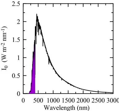
Figure 1.1. Dependence of radiation at the top of the atmosphere on wavelength following the
spectrum given by Gueymard (2004). ... 49
Figure 1.2. Difference between irradiance (a) and actinic flux (b). ... 51
Figure 1.3. a) Erythemal Actium spectrum, Ser; b) its application to obtain erythemal UV radiation, UVER0, for the solar spectrum at the top of the atmosphere in the UV, UV0. ... 52
Figure 1.4. Recommended Sun protection scheme, taken from WHO (2002). ... 53
Figure 1.5. a) Lambertian reflectance; b) reflection by clouds ... 55
Figure 1.6. Definition of absorption: a radiation beam of radiance L crosses a perpendicular layer of thickness dx (without scattering processes). Adapted from Lenoble (1993). ... 56
Figure 1.7. Scattering function. Adapted from Lenoble (1993). ... 58
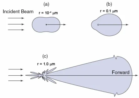
Figure 1.8. Rayleigh scattering (a), Mie scattering (b) and Mie scattering for larger particles (c). ... 60
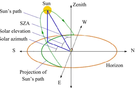
Figure 1.9. Definitions of Solar Zenith Angle (SZA) and other solar parameters. ... 63
Figure 1.10. Ozone in the Chapman cycle. ... 65
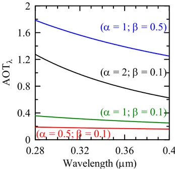
Figure 1.11. Spectral AOT dependence for different values of α and β coefficients. ... 67
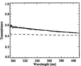
Figure 1.12. Transmittance of a homogeneous cloud layer at Garmisch-Partenkirchen on 22 October, 1995 as a function of wavelength (Seckmeyer et al.,1996; Kylling et al.,1997). ... 72
Figure 1.13. CMF for the actinic flux versus wavelength at several solar zenith angles obtained by Crawford et al. (2003) by a model study with COT = 15 ... 73
Chapter 2
Figure 2.1. UVB-1 YES pyranometer. ... 78Figure 2.2. UVB-1 pyranometer (SN 090503) spectral response measured in one calibration on 1 October 2009 (black circles) and the erythemal actium spectrum (Ser, red line). ... 79
Figure 2.3. Schematic block diagram of the UVB-1 pyranometer. ... 79
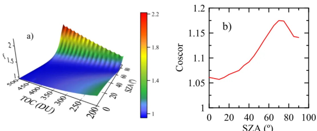
Figure 2.4. a) fn(SZA,TOC) and b) Coscor(SZA) obtained in the calibration performed in the PMOD-WRC of the UVB-1 #090503 on 1 October 2009. ... 81
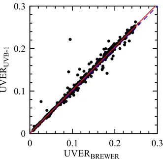
Figure 2.5. Comparison between UVER data obtained with the UVB-1 pyranometer and the BREWER spectroradiometer. ... 82
Figure 2.6. Dependence of the ratio between UVB-1 and BREWER measurements on SZA (a) and TOC (b) values. Blue lines indicate perfect agreement and red lines limit the area to within an error of ±10%. ... 83
Figure 2.8. Comparison of UVER obtained by the UV-MFRSR using seven (a) and four (b) channels and UVB-1 instruments. Red and orange lines are the linear fits and blue dashed lines
indicate the 1:1 line. ... 87
Figure 2.9. BREWER spectroradiometer. ... 88
Figure 2.10. Several processes in BREWER calibration performed at LAMPEDUSA in November 2009. ... 88
Figure 2.11. METCON-DAS actinometer. ... 89
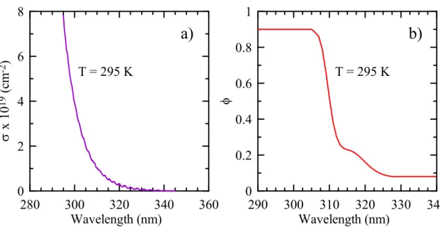
Figure 2.12. Spectral dependence of ozone cross section (a) and quantum yield (b) to determine J(O1D) at a fixed temperature of 295 K. ... 90
Figure 2.13. HATPRO radiometer. ... 91
Figure 2.14. MICROTOPS-II photometer. ... 92
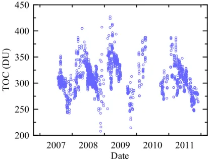
Figure 2.15. TOC database of MICROTOPS-II photometer at the SRSUVA station. ... 94
Figure 2.16. Comparison of TOC obtained by the MICROTOPS-II and OMI instruments. The red line is the linear fit and the blue dashed line indicates the 1:1 line. ... 95
Figure 2.17. YES Total Sky Imager model 440. ... 97
Figure 2.18. Three samples of bad estimation of cloud cover from the TSI’s automatic algorithm. ... 97
Figure 2.19. Three different pictures at the TRISAIA station. ... 98
Figure 2.20. Three different models of pyranometers used in this thesis to record SW radiation. 99 Figure 2.21. Top view of the LIDAR instrument used at the TRISAIA station: CaBLE ... 99
Figure 2.22. VIS-MFRSR YES shadowband radiometer. ... 100
Figure 2.23. Main steps of the Long et al. (2006) algorithm. ... 102
Figure 2.24. Comparison of the fractional sky cover obtained by the algorithms proposed by Long et al. (2006), (SCV)LONG, by Min et al. (2008), (SCV)MIN, and the visual observations, (SCV)VISUAL at the TRISAIA station. ... 105
Figure 2.25. Surface albedo measurements by an aircraft at the TRISAIA station. ... 107
Figure 2.26. COT estimations by Equations (2.18) and (2.19) for different surface albedo (a) and cloud asymmetry factor (b). ... 108
Figure 2.27. Location of the three stations used in this thesis. ... 108
Figure 2.28. SRSUVA station and some of its instruments. ... 109
Figure 2.29. LAMPEDUSA station and some of its instruments. ... 110
Figure 2.30. Some of the instruments at the TRISAIA station. ... 112
Figure 2.31. Definition of radiance, adapted from Lenoble (1993). ... 113
Figure 2.32. Establishing the radiative transfer equation, adapted from Lenoble (1993). ... 114
Figure 2.33. Structure of the uvspec model, adapted from Mayer and Kylling (2005). ... 117
Figure 2.34. Surface albedo (A) values used in the radiative transfer simulations for each station. ... 120
Figure 2.35. Temperature (a) and ozone density (b) profiles for the midlatitude summer (LMS) and standard atmosphere in the US (US). ... 121
Chapter 3
Figure 3.1. Dependence of UV index values on total cloud cover for different solar zenith angles (SZA ≤ 30º, in black, 30º < SZA < 45º, in blue, 45º < SZA < 60º, in purple, and 60º < SZA < 75º, in red) at the SRSUVA (a), TRISAIA (b) and LAMPEDUSA (c) stations. The bars indicate the standard deviation. ... 129 Figure 3.2. Dependence of UV index values on total cloud cover for different solar zenith angles (SZA ≤ 30º, 30º < SZA < 45º, 45º < SZA < 60º, and 60º < SZA < 75º) and TOC values (290 DU < TOC1 < 310 DU and 330 DU < TOC2 < 350 DU) at the SRSUVA station. ... 130 Figure 3.3. Dependence of J(O1D) values on total cloud cover for different solar zenith angles
(SZA ≤ 30º, in black, 30º < SZA < 45º, in blue, 45º < SZA < 60º, in purple, and 60º < SZA < 75º, in red) at the TRISAIA station. The bars indicate the standard deviation. ... 131 Figure 3.4. Look-up-Tables obtained by model (a) and experimental (b) data for UVI values under cloudless conditions at the SRSUVA station. ... 132 Figure 3.5. Look-up-Tables obtained by model (a) and experimental (b) data for UVI values under cloudless conditions at the TRISAIA station. ... 133 Figure 3.6. Look-up-Tables obtained by model (a) and experimental (b) data for UVI values under cloudless conditions at the LAMPEDUSA station. ... 133 Figure 3.7. Comparison between UVI values obtained by the libRadtran Look-up-Table and experimental data under cloudless conditions at the TRISAIA station: a) considering a fixed AOT550nm of 0.25 in the model, b) using the average AOT550nm value for each point. The blue
dashed lines indicate the 1:1 line; the black and red lines are the linear fits. ... 134 Figure 3.8. Dependence of ratio between the UVI estimated with the libRadtran model and that obtained by the measurements on SZA (a) and TOC (b), considering a fixed AOT550nm of 0.25 in
the model (grey points), and using the average AOT550nm value for each point (black points). The
blue dashed lines indicate perfect agreement and the red ones a deviation of ±5%. ... 135 Figure 3.9. Look-up-Tables obtained by model (a) and experimental (b) data for J(O1D) values
under cloudless conditions at the TRISAIA station. ... 136 Figure 3.10. Comparison between J(O1D) values obtained by the libRadtran Look-up-Table and
experimental data under cloudless conditions at the TRISAIA station for three different conditions (see text). The blue dashed line indicates the 1:1 line. ... 137 Figure 3.11. Dependence of the ratio between J(O1D) estimated with the libRadtran model and
the measured one versus SZA (a) and TOC (b), considering in the model a fixed AOT550nm of 0.25
(black points), using the average AOT550nm value for each point (red points), and considering
twice the amount of tropospheric ozone (TCOx2, purple points). Blue dashed lines indicate perfect agreement and the red solid lines a deviation of ±10%. ... 137 Figure 3.12. UVI values in overcast skies (8 octas) as a function of the cloud optical thickness for the SRSUVA (a), TRISAIA (b), and LAMPEDUSA (c) stations. ... 139 Figure 3.13. UVI values in overcast skies (8 octas) as a function of the solar zenith angle for different cloud optical thicknesses for measurements (left panel) and radiative transfer
Figure 3.14. Absolute and relative differences between UVI at SZA = 10º and SZA = 80º as a function of the COT obtained with radiative transfer simulations. ... 141 Figure 3.15. UVI values in overcast skies (8 octas) as a function of the total ozone column for different cloud optical thicknesses for measurements (left panels) and radiative transfer
simulations (right panels) at two fixed intervals of SZA for the TRISAIA database. ... 142 Figure 3.16. Absolute and relative differences between UVI at TOC = 200 DU and TOC = 500 DU as a function of the COT obtained with radiative transfer simulations at SZA = 30º (a) and SZA =60º (b), and with AOT550nm = 0.25. ... 143
Figure 3.17. Simulated UVI values in overcast skies (8 octas) as a function of the aerosol optical thickness at 550 nm for different cloud optical thicknesses for the TRISAIA station at a fixed TOC = 300 DU for two different SZAs: 30º (a) and 60º (b). ... 144 Figure 3.18. Absolute and relative differences between UVI at AOT550nm = 0.05 and AOT550nm =
0.85 as a function of the COT obtained with radiative transfer simulations at SZA = 30º (a) and SZA = 60º (b), and TOC = 300 DU. ... 145 Figure 3.19. J(O1D) values in overcast skies (8 octas) as a function of the cloud optical thickness
for the TRISAIA station. ... 145 Figure 3.20. J(O1D) values in overcast skies (8 octas) as a function of the solar zenith angle for
different cloud optical thicknesses for measurements (left panel) and radiative transfer
simulations (right panel) at a fixed interval of TOC for the TRISAIA database. ... 146 Figure 3.21. J(O1D) values in overcast skies (8 octas) as a function of total ozone column for
different cloud optical thicknesses for measurements (left panels) and radiative transfer
simulations (right panels) at two fixed intervals of SZA for the TRISAIA database. ... 147 Figure 3.22. Simulated J(O1D) values in overcast skies (8 octas) as a function of aerosol optical
thickness at 550 nm for different cloud optical thicknesses for the TRISAIA station at a fixed TOC = 300 DU for two different SZAs: 30º (a) and 60º (b). ... 148 Figure 3.23. Absolute and relative differences between J(O1D) at SZA of 10º and 80º (a), TOC of
200 and 500 DU (b), and AOT550nm of 0.05 and 0.85 (c) as a function of the COT obtained with
radiative transfer simulations. ... 149 Figure 3.24. CMFUVI values (measurements and simulations in grey and orange, respectively) in
overcast skies (8 octas) as a function of cloud optical thickness at the SRSUVA (a), TRISAIA (b), and LAMPEDUSA (c) stations. The green dash and the blue solid lines are fits made with the measured and modelled data, respectively. ... 151 Figure 3.25. CMFUVI = (1 + c1 COT)-1 with the coefficients of Table 3.1 for the three stations
(SRSUVA, TRISAIA and LAMPEDUSA, labelled LAMPE in the legend), for both experimental (solid lines) and model (dashed lines) results. ... 152 Figure 3.26. CMFJ(O1D) values (measurements and simulations in grey and orange, respectively)
in overcast skies (8 octas) as a function of cloud optical thickness at the TRISAIA station. The green dash and the blue solid lines are fits made with the measured and modelled data,
respectively. ... 153 Figure 3.27. CMF = (1 + c1 COT)-1 for UVI and J(O1D) with the coefficients of Table 3.1 and
Chapter 4
Figure 4.1. Irradiance CMF spectral dependence for 0-2 octas (a), and overcast (8 octas, b) cloud cover as a function of the solar zenith angle (SZA) at the LAMPEDUSA station. ... 159 Figure 4.2. Measured (a, c, e) and modelled (b, d, f) CMF versus wavelength as a function of the solar zenith angle for different cloud optical thickness values. Dashed bold lines in the right panels relate to simulations with twice the amount of tropospheric ozone at 30°, 50°, and 70º SZA, respectively in b), d), and f). ... 161 Figure 4.3. Measured (left panels) and modelled (right panels) values of actinic flux CMF versus wavelength as a function of the solar zenith angle for different cloud optical thickness values. . 164 Figure 4.4. CMF for the irradiance (CMFI, dashed lines) and the actinic flux (CMF , solid lines)
calculated with the libRadtran model for COT = 15, TOC = 300 DU and AOT550nm = 0.25 at
several SZAs. ... 165
F
Figure 4.5. Global (left panels) and diffuse (right panels) experimental values of irradiance CMF versus wavelength as a function of the solar zenith angle for different cloud optical thickness values. ... 167 Figure 4.6. Global (solid lines, right panels) and diffuse (dashed lines, left panels) values of irradiance CMF versus wavelength as a function of the solar zenith angle for different cloud optical thickness values evaluated using the libRadtran model. ... 169 Figure 4.7. Evolution of the UVDIRECT(λ)/UVDIFFUSE(λ) ratio under cloudless conditions for two
different solar zenith angles. ... 170 Figure 4.8. Figure 2 at Lindfors and Arola (2008) and the analyzed scenario. ... 172 Figure 4.9. Profiles of air density (a) and pressure (b) for the normal scenario and the DENS option (see text). ... 173 Figure 4.10. Spectral CMF of global (a) and diffuse (b) components for two different scenarios: normal case and the new density profile explained in the test for two different solar zenith angles. ... 174 Figure 4.11. Normalized radiance compared to the maximum value among all the directions between 0º and 90º polar angle at the zenith (solid lines) and 20.5º and 70.5º (dashed lines) of polar angle at SZA = 20º (a, b) and SZA = 70º (c,d), respectively. Cloud-free (a, c) and overcast (b, d) conditions are considered. ... 176 Figure 4.12. The five action spectra used to calculate the BEUVD dose: plant damage (1), erythemal (2), phytoplankton inhibition (3), DNA damage (4), and vitamin D synthesis (5). ... 178 Figure 4.13. (a) Dependence of UV index on cloud optical thickness at two solar zenith angles. Solid lines reflect the real case, and the dashed ones the assumption of constant CMF. (b)
Differences between the two derived values of UVI versus COT. ... 179 Figure 4.14. Differences between the UV irradiance weighted for various biological action spectra calculated with the derived CMF and with constant CMF: (a) plant damage, (b)
Chapter 5
Figure 5.1. CMFUVI as a function of the LWP for different cloud droplet radii. Dots are the
experimental data (different symbols correspond to different days) and lines are the radiative transfer simulations at SZA = 18º (solid lines) and SZA = 75º (dashed lines). ... 185 Figure 5.2. CMFUVI as a function of LWP for different cloud droplet radii and for different cloud
base heights. Dots are the experimental data and solid lines are the radiative transfer simulations at SZA = 18º. ... 187 Figure 5.3. CMFJ(O1D) as a function of the LWP for different cloud droplet radii for three SZA
intervals. Dots are the experimental data (different symbols correspond to different days). In each plot, solid lines refer to results of simulations at the smallest SZA in the range (18° in graph a; 42° in graph b; 63° in graph c), and dashed lines refer to simulations at the largest SZA in the range. ... 188 Figure 5.4. Dependence of modelled CMFJ(O1D) on solar zenith angle for three values of LWP and
two different effective radii: a) 2.5 μm, and b) 10 μm... 190 Figure 5.5. Dependence of CMFUVI (purple lines) and CMFJ(O1D) (red lines) on LWP at 18º, a) and
c), and 75º, b) and d), of SZA for two fixed cloud droplet radii of 2.5 μm, a) and b), and 10 μm, c) and d). ... 191 Figure 5.6. Dependence on SZA of the ratio between diffuse and global components for the UVI (purple line) and J(O1D) (red line) calculated with the libRadtran model for cloudless conditions.
... 192 Figure 5.7. CMF for the global and diffuse spectral irradiances at two wavelengths as a function of LWP for different cloud droplet radii in the SZA interval (18º, 30º). Dots are the experimental data and lines are the radiative transfer simulations at SZA = 18º (solid lines) and SZA = 30º (dashed lines). ... 195 Figure 5.8. CMF for the global and diffuse spectral irradiances at two wavelengths as a function of LWP for different cloud droplet radii in the SZA interval (42º, 54º). Dots are the experimental data and lines are the radiative transfer simulations at SZA = 42º (solid lines) and SZA = 54º (dashed lines). ... 196 Figure 5.9. CMF for the global and diffuse spectral irradiances at two wavelengths as a function of LWP for different cloud droplet radii in the SZA interval (63º, 75º). Dots are the experimental data and lines are the radiative transfer simulations at SZA = 63º (solid lines) and SZA = 75º (dashed lines). ... 197 Figure 5.10. CMF for the actinic flux at two wavelengths as a function of LWP for different cloud droplet radii in the three SZA intervals. Dots are the experimental data and lines are the radiative transfer simulations at the smallest (solid lines) and highest (dashed lines) SZAs in each panel. ... 199 Figure 5.11. CMF for the global irradiance (CMFI, purple lines) and actinic flux (CMF , red
lines) at SZA = 18º (solid lines) and SZA = 63º (dashed lines) at 304.7 nm, a) and c), and 367.2 nm, b) and d), for fixed reff of 5, a) and b), and 15, c) and d), μm. ... 200
Figure 5.12. Spectral ratios between diffuse and global components for the irradiance (purple lines) and actinic flux (red lines) at 18º (solid lines) and 75º (dashed lines) calculated with the libRadtran model for cloudless conditions. ... 201
Chapter 6
Figure 6.1. Frequency of overcast events as a function of their length in hours. ... 206 Figure 6.2. Vertical distribution of Aerosol Backscatter Ratio at 532 nm on 30 May 2010 at the TRISAIA station. ... 207 Figure 6.3. Ozone profiles in the standard mid-latitude summer atmosphere (red line) and in the new profile to produce more realistic values of ozone at surface (blue line). ... 208 Figure 6.4. Three-day trajectories ending at the TRISAIA station at 14:00 UT 30 May 2010 for three different heights: 500 (red), 1500 (blue), and 2500 (green) m a.s.l. Source: NOAA Air Resources Laboratory (ARL) and READY website (http://ready.arl.noaa.gov) ... 209 Figure 6.5. a-b) Comparison between modelled (green lines) and measured (black lines) spectral CMF values. c-d) Spectral ratios between CMF calculated by the libRadtran model and
experimental data; horizontal grey lines indicate a difference of 5% (dashed) and perfect agreement (solid). Left and right panels correspond to global and diffuse components,
respectively. ... 211 Figure 6.6. a) Comparison between measured (black lines) and modelled (green lines) spectral actinic flux CMF values. b) Spectral ratios between CMF calculated by the libRadtran model and experimental data; horizontal grey lines indicate a difference of 5% (dashed) and perfect
agreement (solid). ... 212 Figure 6.7. Spectral CMF for the irradiance (purple line) and the actinic flux (red line) obtained by experimental (a) and model (b) data. ... 212 Figure 6.8. Heights at which irradiances are simulated with the libRadtran for the case study. 213 Figure 6.9. Spectral CMFaer/CMFNOaer ratio for global (a) and diffuse (b) components at five
different heights. ... 214 Figure 6.10. Spectral ratios of Equation (6.1) for global (a) and diffuse (b) components at the surface for a desert dust aerosol layer. ... 215 Figure 6.11. Spectral CMFaer/CMFNOaer ratio for global (a) and diffuse (b) components at five
different heights considering a maritime clean aerosol layer. ... 216 Figure 6.12. Spectral ratios of Equation (6.1) for the global (a) and diffuse (b) components at the surface for a maritime clean aerosol layer. ... 216 Figure 6.13. a-b) Spectral CMFaer/CMFNOaer ratio for global (a) and diffuse (b) components at
Figure 6.15. Sensitivity analysis of the CMF for global (solid lines) and diffuse (dashed lines) components for two aerosol optical thickness values. ... 221 Figure 6.16. Sensitivity analysis of the CMF for global (solid lines) and diffuse (dashed lines) components for two aerosol asymmetry factor values. ... 222 Figure 6.17. Ratios between the simulated irradiances, global (a) and diffuse (b), for g = 0.65 and g = 0.95 in cloudless (blue lines) and overcast (black lines) conditions. ... 223 Figure 6.18. Sensitivity analysis of the CMF for global (solid lines) and diffuse (dashed lines) components for two aerosol single scattering albedo values. ... 223 Figure 6.19. Ratios between the simulated irradiances, global (a) and diffuse (b), for ω0 = 0.6
and ω0 = 0.99 in cloudless (blue lines) and overcast (black lines) conditions. ... 224
Figure 6.20. Sensitivity analysis of the CMF for global (solid lines) and diffuse (dashed lines) components for two cloud asymmetry factor values. ... 226 Figure 6.21. Sensitivity analysis of the CMF for global (solid lines) and diffuse (dashed lines) components for two cloud single scattering albedo values. ... 227 Figure 6.22. Diagram for the two situations analyzed with regard to cloud geometric thickness. ... 228 Figure 6.23. Spectral CMF dependence for global (solid lines) and diffuse (dashed lines)
Chapter 1
Table 1.1. Some photochemical reactions occurring in the atmosphere in the UV range. ... 53
Chapter 2
Table 2.1. Statistical indexes of the comparison between UVB-1 and BREWER measurements of UVER carried out at Lampedusa Island in 2010 during 56 days: n is the number of data, UVERave
represents the average of all the experimental data, MBE and RMSE are the mean bias error and the root mean square error, respectively, and Wi is the percent of cases whose deviation falls
below the ±i% difference. ... 83
Table 2.2. Coefficients of Equation (2.6) obtained for the UV-MFRSR. ai coefficients are unitless,
while bi are in m2 nm W-1. ... 86
Table 2.3. Statistical indexes of the comparison between UVER data obtained by the UV-MFRSR using seven and four channels and the UVB-1 pyranometer. n is the number of data, UVERave
represents the average of all the experimental data, MBE and RMSE are the mean bias error and the root mean square error, respectively, and Wi is the number of cases falling below the ±i%
error. ... 87
Table 2.4. Statistical indexes of the comparison between TOC data obtained by the MICROTOPS-II and OMI and BREWER instruments. n is the number of data, TOCave represents the average of
all the experimental data, MBE and RMSE are the mean bias error and the root mean square error, respectively, and Wi is the number of cases falling below the ±i% error. ... 96
Table 2.5. SRSUVA station instruments used, the variables they record and the time period used for the thesis. ... 110
Table 2.6. LAMPEDUSA station instruments used, the variables they record and the time period used for the thesis. ... 111
Table 2.7. TRISAIA station instruments used, the variables they record and the time period used for the thesis. ... 112
Chapter 3
Table 3.1. c1 coefficient of Equation (3.1), its standard error (SE), and correlation coefficient (r)
for the three stations. ... 152
Table 3.2. c1 coefficient of Equation (3.1) but for the CMFJ(O1D), its standard error (SE), and the
Chapter 4
Table 4.1. Number of UV spectra at 8 octas for the three ranges of cloud optical thickness (COT) as a function of the solar zenith angle (SZA) at the LAMPEDUSA station. ... 162
Table 4.2. Number of actinic flux spectra at 8 octas for the three values of COT as a function of the SZA at the TRISAIA station. ... 163
Table 4.3. Number of irradiance (global and diffuse) spectra at 8 octas for the three values of COT as a function of the SZA at the TRISAIA station. ... 166
Table 4.4. Correction factors for taking into account the 363.5-400 nm range in UVI calculations. ... 179
Chapter 6
Table 6.1. Atmospheric and meteorological conditions recorded at 14:00h UT 30 May 2010 at the TRISAIA station. ... 208
Manuscripts
Mateos, D., Bilbao, J., Kudish, A.I., Parisi, A.V., Carbajal, G., di Sarra, A., Román, R., and de Miguel, A., 2012, Validation of satellite erythemal radiation retrievals using ground-based measurements in five Countries, Remote Sensing of Environment, Under Review.
Román, R., Mateos, D., de Miguel, A., Bilbao, J., Pérez-Burgos, A., Rodrigo, R., and Cachorro, V.E., 2012, Atmospheric effects on the ultraviolet erythemal and total shortwave solar radiation in Valladolid, Spain, Óptica Pura y Aplicada 45(1), 17‐21.
Mateos, D., Román, R., Bilbao, J., de Miguel, A., and Pérez‐Burgos, A., 2012, Cloud modulation of shortwave and ultraviolet solar irradiances at surface, Óptica Pura y Aplicada 45(1), 29‐32.
Bilbao, J., Román, R., de Miguel, A., and D. Mateos, 2011, Long-term solar erythemal UV irradiance data reconstruction in Spain using a semi-empirical method, Journal of Geophysical Research 116, D22211, doi:10.1029/2011JD015836.
De Miguel, A., Bilbao, J., Román, R., and Mateos, D., 2011, Measurements and attenuation of erythemal radiation in Central Spain, International Journal of Climatology, Published on-line, doi: 10.1002/joc.2319.
Mateos, D., di Sarra, A., Meloni, D., Di Biagio, C., and Sferlazzo, D.M., 2011, Experimental determination of cloud influence on the spectral UV radiation and implications for biological effects, Journal of Atmospheric and Solar-Terrestrial Physics 73, 1739–1746, doi:10.1016/j.jastp.2011.04.003.
de Miguel, A., Mateos, D., Bilbao, J., and Román, R., 2011, Sensitivity analysis of ratio between ultraviolet and total shortwave solar radiation to cloudiness, ozone, aerosols and precipitable water, Atmospheric Research 102, 136–144, doi:10.1016/j.atmosres.2011.06.019.
de Miguel, A., Román, R., Bilbao, J., and Mateos, D., 2011, Evolution of erythemal and total shortwave solar radiation in Valladolid, Spain: Effects of atmospheric factors, Journal of Atmospheric and Solar-Terrestrial Physics 73, 578–586, doi:10.1016/j.jastp.2010.11.021.
Bilbao, J., Mateos, D., and de Miguel, A., 2011, Analysis and cloudiness influence on UV total irradiation, International Journal of Climatology 31 (3), 451–460, doi:10.1002/joc.2072.
Mateos, D., de Miguel, A., and Bilbao, J., 2010, Empirical models of UV total radiation and cloud effect study, International Journal of Climatology 30, 1407–1415, doi:10.1002/joc.1983.
Mateos, D., Bilbao, J., de Miguel, A., and Pérez-Burgos, A., 2010, Dependence of ultraviolet (erythemal and total) radiation and CMF values on total and low cloud covers in Central Spain, Atmospheric Research 98, 21–27, doi:10.1016/j.atmosres.2010.05.002.
Conferences
Mateos, D., di Sarra, A., Bilbao, J., Cacciani, M., Casasanta, G., Meloni, D., Pace, G., and de Miguel, A., Experimental and modelled characterization of diffuse spectral UV irradiance under cloudy conditions: impact of aerosol properties, European Aerosol Conference, Granada Spain, 2-7 September 2012.
Mateos, D., di Sarra, A., Bilbao, J., Pace, G., Meloni, D., de Miguel, A., Casasanta, G., and Min, Q., Wavelength dependence of diffuse and total Cloud Modification Factors for UV irradiance and actinic flux for different cloud optical and microphysical properties, International Radiation Symposium, Berlin, Germany, 6-10 August 2012.
Mateos, D., Bilbao, J., Kudish, A.I., Parisi, A.V., Carbajal, G., di Sarra, A., Román, R., and, de Miguel, A., Daily erythemal radiation validation of satellite retrievals using 14 ground-based stations in both hemispheres, International Radiation Symposium, Berlin, Germany, 6-10 August 2012.
Román, R., Bilbao, J., de Miguel, A., and Mateos, D., Analysis of erythemal radiation evolution along twenty years in Central Spain, International Radiation Symposium, Berlin, Germany, 6-10 August 2012.
Mateos, D., Bilbao, J., de Miguel, A., Román, R., and Pérez-Burgos, A., Satellite Radiation Retrieval Validation in Spain: Impact of Ozone, Clouds and Aerosols, V Reunión Española de Ciencia y Tecnología de Aerosoles – RECTA 2011, Madrid, Spain, 27-29 June 2011.
Román, R., Bilbao, J., de Miguel, A., Mateos, D., and Pérez-Burgos, A., Influence of aerosol optical depth on ultraviolet erythemal radiation, V Reunión Española de Ciencia y Tecnología de Aerosoles – RECTA 2011, Madrid, Spain, 27-29 June 2011.
Mateos, D., Bilbao, J., de Miguel, A., and Román, R., Aerosol, cloud and water effects on the relationship between UV and total shortwave radiant fluxes, WAVACS-COST winter school Water Vapour in the Climate System, Venice, Italy, 6-12 February 2011.
Pérez-Burgos, A., De Miguel, A., Bilbao, J., and Mateos, D., Prediction of Solar Irradiance and Illuminance Using REST2 Model, EuroSun 2010, Graz, Austria, 28 September – 1 October 2010.
Mateos, D., de Miguel, A., Bilbao, J., and Román, R., 2010, What effect does the presence of clouds on UV solar radiation attenuation?, 37th Annual European Meeting on Atmospheric Studies by Optical Methods, Valladolid, Spain, 23-27 August 2010.
de Miguel, A., Mateos, D., Bilbao, J., Román, R., and Pérez-Burgos, A., 2010, Dependence on cloudiness of CMF values in the UV range, 37th Annual European Meeting on Atmospheric Studies by Optical Methods, Valladolid, Spain, 23-27 August 2010.
de Miguel, A., Román, R., Mateos, D., Bilbao, J., Pérez-Burgos, A., Cachorro, V.E., and Rodrigo, R., Atmospheric effects on the erythemal ultraviolet and total shortwave solar radiation in Valladolid, Spain, 37th Annual European Meeting on Atmospheric Studies by Optical Methods, Valladolid, Spain, 23-27 August 2010.
Mateos, D., de Miguel, A., and Bilbao, J., Climatological study of total ozone column in central Spain, MOCA-09: IAMAS Simposia, Montreal, Canada, 19-29 July 2009.
Bilbao, J., de Miguel, A., and Mateos, D., Daily solar UV-B radiation evaluated from meteorological variables, MOCA-09: IAMAS Simposia, Montreal, Canada, 19-29 July 2009.
Mateos, D., Bilbao, J., and de Miguel, A., Empirical models of ultraviolet total solar radiation, MOCA-09: IAMAS Simposia, MOCA-09: IAMAS Simposia, Montreal, Canada, 19-29 July 2009.
Mateos, D., de Miguel, A., and Bilbao, J., The cloudiness effect on UV radiation, EGU General Assembly 2009, Vienna, Austria, 19-24 April 2009.
Mateos, D., de Miguel, A., and Bilbao, J., Climatology of Ultraviolet Global Solar Irradiation, 6º Simpósio de Meteorologia e Geofísica da APMG / 10º Encontro Luso-Espanhol de Meteorologia, Aldeia dos Capuchos, Portugal, 16-18 March 2009.
Mateos, D., Bilbao, J., de Miguel, A., and Cachorro, V.E., Comparison of total ozone column, precipitable water and aerosol optical thickness in central Spain, EGU General Assembly 2008, Vienna, Austria, 13-18 April 2008.
AEMet Spanish Meteorological Agency AERONET Aerosol RObotic NETwork
CIE International Commission on Illumination
COST 726 Long Term changes and Climatology of UV Radiation over Europe DAS Diode Array Spectrometer
DU Dobson Unit
ENEA Agenzia Nazionale per le Nuove Tecnologie, l’Energia e lo Svilippo Economico Sostenibile
GAW Global Atmospheric Watch
GOME Global Ozone Monitoring Experiment HATPRO Humidity and Temperature Profiler
ICNIRP International Commission on Non-Ionizing Radiation Protection INTA National Institute for Aerospace Technology
IPCC Intergovernmental Panel on Climate Change
LAMPEDUSA Referred to the ENEA station placed in Lampedusa island LIDAR Light Detection and Ranging
LUT Look-Up-Table
GMT Greenwich Mean Time
MODIS Moderate Resolution Imaging Spectroradiometer NASA National Aeronautics and Space Administration NCEP National Centres for Environmental Prediction
OMI Ozone Monitoring Instrument
PMOD-WRC World Radiometric Centre RTE Radiative Transfer Equation
SRSUVA Solar Radiometric Station of the University of Valladolid TOMS Total Ozone Mapping Spectrometer
TRISAIA Referred to the measurement campaign the ENEA-Trisaia centre TSI Total Sky Imager of Yankee Environmental Systems model 440 UNEP United Nations Environment Programme
UVA University of Valladolid
UV-MFRSR Multifilter Shadowband Radiometer for the ultraviolet range VIS-MFRSR Multifilter Shadowband Radiometer for the visible range WHO World Health Organization
WMO World Meteorological Organization YES Yankee Environmental Systems, Inc
α Ångström exponent
β Ångström turbidity
Γ Day angle (degree)
δ Declination (degree)
ε Temperature correction function
λ Wavelength (nm)
Λ Latitude (degree)
μ0 Cosine of the solar zenith angle
ρw Water density (g m-3)
σ Absorption cross section of ozone (cm2 molec-1)
τ Total optical thickness
τa,s Absorption (a) and scattering (s) optical thickness
υ Frequency (s-1)
Quantum yield of the ozone photodissociation (molec quanta-1)
Φ Solar azimuth angle (degree)
ω0 Single scattering albedo
Solar hour angle (degree)
A Surface albedo
Ar Area AOT Aerosol Optical Thickness
AOTλ Aerosol Optical Thickness at a wavelength of λ BEUVD Biologically effective UV doses
CMF Cloud Modification Factor or cloud transmittance
CMFaer Cloud Modification Factor for normal conditions (aerosol considered)
CMFDIFFUSE Cloud Modification Factor for the diffuse component
CMFF Cloud Modification Factor for the actinic flux (global component)
CMFGLOBAL Cloud Modification Factor for the global component
CMFI Cloud Modification Factor for the irradiance (global component)
CMFJ(O1D) Cloud Modification Factor for the ozone photolysis rate
CMFNoaer Cloud Modification Factor for an aerosol-free atmosphere
CMFUVI Cloud Modification Factor for the ultraviolet index
CosCor Cosine correction function COT Cloud Optical Thickness CRE Cloud Radiative Effect (W m-2) dn Day number of the year
E0 Sun-Earth distance correction
F Actinic flux (quanta cm-2 s-1, can be defined spectrally)
g Asymmetry factor
h Height (m)
hcld Height of the cloud base (m)
I Irradiance (W m-2, can be defined spectrally)
I0 Radiation at the top of the atmosphere (W m-2, can be defined
spectrally)
J(O1D) Ozone photolysis rate (s-1)
ka,e,s Absorption (a), extinction (e) and scattering (s) coefficients (m-1)
L Radiance (W m−2 sr−1, can be defined spectrally) LWC Liquid Water Content (g m-3)
LWP Liquid Water Path (g m-2)
m Relative optical air mass
M Number of UV-MFRSR channels
MBE Mean Beas Error
n Number of data
P Function of phase
Qe Mie scattering effienciency factor
r Correlation coefficient
R Mean Earth radius (~6371 km)
reff Effective radius of cloud droplets (μm)
RMSE Root Mean Square Error
T Temperature (K)
TCO Tropospheric Column Ozone (DU) TOC Total Ozone Column (DU)
S Action spectrum
SCV Fractional Sky Cover
SE Standard error
Ser Erythemal action spectrum
SW Shortwave radiation (W m-2, can be defined spectrally) SZA Solar Zenith Angle (degree)
UV Ultraviolet radiation (W m-2, can be defined spectrally) UV-A Ultraviolet type A radiation (W m-2, can be defined spectrally)
UV-B Ultraviolet type B radiation (W m-2, can be defined spectrally) UV-C Ultraviolet type C radiation (W m-2, can be defined spectrally) UVER Erythemal Ultraviolet Radiation (W m-2, can be defined spectrally)
Due to the decrease in total ozone recorded in recent decades, UV radiation levels at the surface have increased. This, together with the effects this radiation causes on atmospheric chemistry and the biosphere, has led to the need to monitor the UV radiation field (both irradiance and actinic flux). Spectral and integrated quantities of the two variables are usually employed. UV irradiance is usually represented with the UV index, UVI, which describes the UV radiation levels at the surface that produce erythema or sunburn on human skin. One key reaction in the chemistry of the troposphere is ozone photolysis, for which the rate of this reaction, J(O1D), is used. The main factors involved in the attenuation of UV radiative flux on the Earth's surface are solar elevation, cloudiness, ozone, aerosol, surface albedo, and altitude. Cloud effect on solar UV radiative flux has only been partially explored due to the lack of measurements of cloud properties, which show a large temporal and spatial variability and determine the final levels of radiation at the surface. The main aim of this work is therefore to characterize radiative flux under overcast conditions.
A large number of instruments located at three different European stations were involved in the analysis described in this thesis. These instruments provided measurements of global and diffuse spectral irradiances and spectral actinic flux in the UV range, UVI, J(O1D), cloud optical thickness (COT), liquid water path (LWP), effective radius of cloud droplets (reff), total ozone column (TOC), cloud cover, cloud
base and top heights, and aerosol optical thickness (as well as its vertical distribution). Radiative transfer simulations with the libRadtran library have been carried out as realistically as possible using input such as aerosol and cloud properties, temperature and pressure profiles, and surface albedo.
Characterization of UVI and J(O1D) under overcast conditions was carried out by means of experimental and model data. The influence of solar zenith angle (SZA) and TOC is relevant under overcast conditions, while the aerosol effect is only relevant for the J(O1D). As the cloud modification factor (CMF) was calculated to investigate cloud effect, a good estimation under cloudless conditions was required. The CMFs for the UVI and J(O1D) are studied as a function of COT. Experimental and model results are very similar, and no significant differences between CMFUVI and CMFJ(O1D) are observed. The
relationship between CMF and COT can be approximated with CMF = (1 + c1 COT)-1.
nm, and decreases beyond this wavelength with a weak SZA effect. Beyond 320 nm, the CMF for the actinic flux shows three different behaviours: slightly increasing behaviour at low SZA, decreasing behaviour at moderate SZA, and a strongly decreasing behaviour at high SZA. The CMF for diffuse irradiance always increases with wavelength. The processes involved in UV radiation attenuation under cloud presence are scattering on molecules, and aerosol and cloud particles, and absorption by ozone. These processes lead to the following mechanisms: multiple reflections between the cloud and the atmosphere above; enhanced ozone absorption; dependence on SZA and wavelength in attenuation; and photons arriving from the zenith direction due to the Umkehr effect (more effectively for the shorter wavelengths). Finally, these effects have to be considered when biological effects are calculated using the CMF. If the CMF is taken as wavelength-independent, a notable overestimation of UV radiation occurs.
In the analysis considering cloud microphysical properties, droplets with a smaller effective radius cause higher attenuation in the overcast scenario. With regard to the different behaviour between irradiance and actinic flux, irradiance is more strongly attenuated at low SZA, and the actinic flux shows the smallest values of CMF at high SZA. These facts can be explained by the different weight of the direct and diffuse components.
Resumen
El descenso de la columna de ozono registrado en las últimas décadas ha provocado un aumento de los niveles de radiación UV en superficie. Debido a este hecho, y sabiendo que esta radiación produce efectos sobre la química de la atmósfera y sobre la biosfera, ha sido necesaria la monitorización del campo radiativo en el intervalo del UV, tanto del flujo actínico como de la irradiancia. Estas dos variables se han medido tanto en su régimen espectral como integrado. Una de las variables que representa la irradiancia UV es el índice UV, UVI, que describe los niveles de esta radiación en superficie que producen eritema o quemadura solar en la piel humana. Con respecto al flujo actínico, se estudia la velocidad de fotólisis del ozono, J(O1D). Los principales factores que modulan el flujo radiativo en el UV que llega a la superficie terrestre son la elevación solar, la nubosidad, el ozono, el aerosol, al albedo superficial, y la altitud. Sin embargo, el efecto de las nubes sobre el flujo radiativo no es del todo conocido debido a la carencia de medidas de propiedades de nubes, que muestran una gran variabilidad tanto espacial como temporal, y que van a determinar los niveles finales de radiación en superficie. Por lo tanto, el principal objetivo de este trabajo es caracterizar el flujo radiativo bajo
condiciones de cielos totalmente cubiertos.
Un gran número de instrumentos han sido necesarios en la realización de esta tesis doctoral en tres estaciones europeas. Se han realizado medidas de la irradiancia espectral (componente global y difusa), del flujo actínico espectral, del UVI y J(O1D), del espesor óptico de las nubes (COT), del contenido de agua líquida (LWP), del radio efectivo de las gotas de las nubes (reff), de la columna de ozono (TOC), de la cubierta, base y cima de las
nubes, del espesor óptico de aerosoles (y su distribución vertical). Se han utilizado también simulaciones con el modelo de transferencia radiativa libRadtran, lo más precisas posibles considerando en las entradas propiedades de nubes y aerosoles, el tipo de atmósfera, el albedo superficial, entre otros.
La caracterización del UVI y J(O1D) en condiciones de cielos totalmente cubiertos
significativas entre el CMFUVI y el CMFJ(O1D). La relación entre el CMF y el COT se
puede establecer como CMF = (1 + c1 COT)-1.
Con respecto a la dependencia espectral (determinada de dos formas distintas usando el COT y medidas de propiedades microfísicas de nubes), los CMFs para la irradiancia global y difusa y el flujo actínico tienen diferentes tendencias. El CMF para la componente global de la irradiancia aumenta hasta los 320 nm, y decrece a partir de esta longitud de onda con un efecto del SZA no muy marcado. El CMF para el flujo actínico, por encima de los 320 nm, presenta tres tendencias: un ligero aumento para bajos SZAs, un decrecimiento para moderados SZAs, y una fuerte tendencia decreciente para altos SZAs. El CMF para la irradiancia difusa aumenta con la longitud de onda. Los fenómenos involucrados en la atenuación de la radiación UV en presencia de nubes son la dispersión sobre moléculas y partículas de aerosol y nubes, y la absorción por el ozono. Estos procesos provocan los siguientes mecanismos: reflexiones múltiples entre la nube y la atmósfera de encima, una mayor absorción por ozono, una dependencia con el SZA y la longitud de onda en la atenuación, y fotones llegando desde el zenit por el efecto Umkehr (más efectivo para las longitudes de onda más pequeñas). Estos efectos se tienen que tener en consideración cuando se están calculando los efectos biológicos, puesto que si se supone un CMF constante con la longitud de onda, se produce una importante sobreestima de la radiación UV.
En el análisis realizado con las propiedades microfísicas de nubes, las gotas con un radio efectivo más pequeño van a producir una mayor atenuación de los flujos radiativos en el escenario de cielos totalmente cubiertos. Con respecto al diferente comportamiento entre la irradiancia y el flujo actínico, mientras que la irradiancia es más fuertemente atenuada para bajos SZAs, el flujo actínico muestra los valores más pequeños de CMF a altos SZAs. Esto se debe a la diferente definición de las dos variables, y por lo tanto, al diferente peso de las componentes directa y difusa.
Introduction, Objectives and Thesis Structure
I.1. Introduction
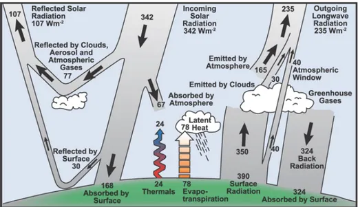
The climate system is defined as an interactive system consisting of the atmosphere, land, snow, and ice surfaces, oceans and other bodies of water, and living things (IPCC, 2007). It is powered by solar radiation mainly in the shortwave range up to 3000 nm. Yet, not all the radiation reaching the top of the Earth’s atmosphere is absorbed; ~30% is reflected back to space by clouds, aerosol particles or Earth’s surfaces, mainly those with high albedo (snow, ice, and deserts). The other ~70% is absorbed by the Earth’s surface and the atmosphere. To balance incoming radiation, the same amount of energy is emitted from the Earth as longwave radiation. The energy is transported all around the Earth and is used for such purposes as water evaporation. Figure I.1 shows the main processes influencing this energy balance. As can be seen in the figure, clouds are the main factor involved in modulating the energy balance (Ramanathan et al., 1989). Clouds can affect the energy balance by reflecting solar radiation back to space (albedo effect of clouds) and by trapping infrared radiation emitted by the surface and the lower troposphere (greenhouse effect of clouds). The relationship between the two effects depends on many factors, including cloud microphysical properties (IPCC, 2007).
Solar ultraviolet (UV) radiation, 100–400 nm, represents only a small percentage of the total solar energy reaching the top of the atmosphere. Yet, UV is the most energetic radiation reaching the surface and exerts a significant influence on the biosphere. The ozone reduction reported in the early 1980s led to an increase in solar UV radiation at the surface. However, over the last 20 years a recovery in ozone values has been observed. Several studies have analyzed these trends and future scenarios (e.g., Weatherhead and Andersen, 2006; WMO, 2011). The UV-B range, 280-315 nm, is of great biological importance since photons from these wavelengths may damage deoxyribonucleic acid (DNA) molecules and certain proteins of living organisms. Not all effects are harmful, however. UV-B radiation is essential for the synthesis of vitamin D in the human body, which has beneficial effects and helps prevent certain diseases. UV radiation is also important for tropospheric chemistry as it is involved in important photochemical reactions, such as nitrogen dioxide photolysis, ozone, and formaldehyde. Changes in the tropospheric composition can influence the stratosphere through interactions between both layers. Finally, links have been established between changes in UV radiation and climate change (Bais et al., 2007).
Monitoring UV radiation at the Earth’s surface requires detailed instrument characterization and accurate calibration in order to provide high quality UV radiation data. High maintenance costs mean that UV radiation measurement networks are confined to certain areas (e.g., Fioletov et al., 2002; Cede et al., 2004). In recent years, the use of instruments onboard satellites has also addressed the assessment of UV levels at the surface (e.g., Fioletov et al., 2004; Meloni et al., 2005; Ialongo et al., 2011). A study into the validation of satellite UV retrievals was carried out, although this topic was not one of the objectives of the thesis (Mateos et al., 2012a).
The main factors modulating UV radiation levels at the surface are: Sun-Earth geometry, clouds, ozone, aerosol, surface albedo, and altitude. In particular, clouds dominate any other atmospheric variable as a source of surface UV variability resulting in either a reduction or an increase in UV radiation. This depends on cloud cover and the position in relation to the Sun, cloud optical thickness, and microphysical properties. These variables present large temporal and spatial variability, which prevents cloud effect from being determined.