Master Erasmus Mundus in
Mediterranean Forestry and Natural Resources
(MEDFOR)
Tree biomass and biodiversity
relationship in a mixed Mediterranean
forest in Spain
Student: Narangarav Dugarsuren
Co-advisors: Prof. Felipe Oviedo Bravo
Ing. Cristobal Ordonez Alonso
INDEX
LIST OF FIGURES ... 4
LIST OF TABLES ... 4
RESUMEN ... 5
ABSTRACT ... 5
1. - INTRODUCTION ... 6
2. - OBJECTIVES... 8
3. - MATERIAL AND METHODS ... 8
3.1. Study site ... 8
3.2. Biomass estimation ... 10
3.3. Tree species diversity estimation ... 11
3.3.1. Species richness indices ... 11
3.3.1.1. Simpson Diversity index (1-D) ... 11
3.3.1.2. Shannon index ... 11
3.3.1.3. Berker-Parker index (D) ... 12
3.3.1.4. Evenness index (E) ... 12
3.3.2. Species intermingling ... 12
3.3.2.1. Species segregation (S) index ... 12
3.3.2.2. Mingling (Mi) index ... 13
3.3.2.3. Spatial diversity status (MS) ... 14
3.3.3. Spatial structural indices ... 15
3.3.3.1. Uniform Angle Index (W)... 16
3.3.3.2. Aggregation index R ... 16
3.3.3.3. Height Differentiation index (TH) ... 16
3.3.3.4. Vertical species profile (A)... 17
3.4. Statistical analysis ... 17
4. - RESULTS ... 19
5. - DISCUSSION ... 23
6. - CONCLUSIONS ... 24
7. - AKNOWLEDGEMENTS ... 24
8. - REFERENCES ... 25
LIST OF FIGURES
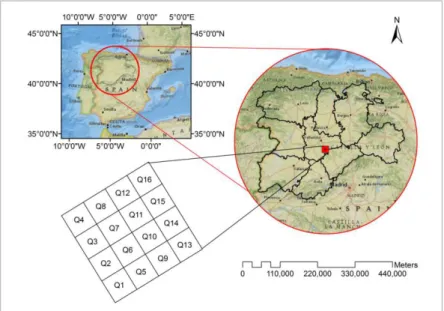
Figure 1.Study area location of Marteloscope of Llano de San Marugan (Valladolid,
Spain) ... 9
Figure 2. Workflow for the study of tree biomass and diversity relationship ... 9
Figure 3. Description and calculation of Mingling index (Mi), Spatial diversity status (MS) and Uniform Angle index (Wi) and corresponding likelihood values for structure unit of 4 neighbors around the reference i tree: a, b, c, d are the tree species types ; 𝜽 are angles between adjacent neighbor trees; 𝜽𝒔 is a standard angle (which is equal to 360/4 for 4 neighbor trees) (Adapted from Gadow & Hui, 2002) ... 15
LIST OF TABLES Table 1. Biomass allometric equations by species ... 10
Table 2. Categorization of indices ... 11
Table 3. Descriptions of variables for S index calculation ... 13
Table 4. Fitting models and their predictor variable reference ... 19
Table 5. Parameter estimates for biomass from selected models at community level ... 21
RESUMEN
La biomasa de árboles y su relación con la diversidad en bosques mixtos se ha convertido en uno de los temas de investigación más interesantes para los ecólogos en las últimas décadas debido a la importancia de los bosques mixtos para una mejor provisión de servicios ecosistémicos. La pregunta “¿Producen los bosques mixtos más a medida que aumenta la diversidad de árboles?” Ha sido objeto de muchos estudios que llevan a resultados no concluyentes. Este estudio se realizó para contrastar el resultado de estudios anteriores mediante la investigación de la biomasa de árboles y la relación de diversidad en un rodal mixto de bosque mediterráneo (Llano de San Marugan, España), tanto a nivel de masa como de árbol individual. Se analizaron diversos modelos que se ajustaron a partir de ecuaciones de regresión lineal y no lineal para determinar la relación entre la biomasa de los árboles y la diversidad. Se utilizaron 10 índices de diversidad que se pueden clasificar en 3 categorías: índices de riqueza de especies (Sm, Sn, D, E); Índices de composición / mezcla de especies (Mi, MS, S); Los índices estructurales verticales (W, A, TH) como variables predictoras de los modelos con el objeto de caracterizar diferentes estructuras de diversidad en el rodal. Nuestro resultado reveló que la relación entre la biomasa y la diversidad de árboles varía entre las especies. Una combinación de la relación negativa del índice D-Berker-Parker (abundancia de especies dominantes) y la relación positiva de TH (heterogeneidad de la altura) explica la variación de la biomasa a nivel rodal y para Pinus pinea. La biomasa de las especies de Quercus (Quercus faginea y Quercus ilex) se relaciona positivamente con la proporción de especies en área basimétrica (Gp); los índices de diversidad probados no mostraron ninguna relación con la biomasa de las especies del género Quercus.
Palabras clave: diversidad de especies arbóreas, índices de diversidad, riqueza específica, composición específica, estructura vertical del rodal.
ABSTRACT
Tree biomass and diversity relationship in mixed forest has become one of the attractive research subjects for ecologist in recent decades due to an importance of multicultural mixed forest for better provision of goods and services than monoculture. The questions “Does mixed forest produce more productive and the productivity increase as tree diversity increases?” have been subject of many researches that lead to two contrast results. This study was conducted to contrast the result of previous studies by investigating the tree biomass and diversity relation in Mediterreanean multicultural mixed stand, Llano de San Marugan, Spain, at stand and individual species level. A variety of models that developed from linear and nonlinear regression equations were employed to reveal tree biomass and diversity relation. 10 diversity indices that falls in 3 categories: species richness indices (Sm, Sn, D, E); species compositional/mingling indices (Mi, MS, S); vertical structural indices (W, A, TH) were used as predictor variables for the models to characterize different structure of diversity in the stand. Our result revealed that tree biomass and diversity relation varies among species. A combination of negative relation of D- Berker-Parker index (abundance of dominant species) and positive relation of TH (height heterogeneity) explains the variation of biomass at community level and for Pinus pinea. Biomass of Quercus species (Quercus faginea and Quercus ilex) was positively related with basal area proportion of species (Gp); the tested diversity indices didn’t show any relation with biomass of Quercus
species and Juniperus thurifera as concerned by metrics and models in this study.
1. - INTRODUCTION
Mediterranean forests are characterized by a remarkable set of features that make them naturally and aesthetically attractive, but also quite fragile (Scarascia-Mugnozza et al., 2000). Mediterranean forest is a multi-functional, providing a wide range of goods and services for society ranging from products with high market value (fuelwood, cork, mushroom, pinecones etc) and non-market value ecosystem services (soil and landscape protection, water regulation, biodiversity conservation, carbon dioxide fixation, recreation, aesthetic view etc). The latter is more significant than their productive value, especially their significant role for carbon sequestration (del Río et al., 2017). One of notable characteristics of Mediterranean forests is its rich biodiversity, reflected by high genetic variability, exemplified by the large number of tree species in comparison to Nordic forests resulting from the survival of many conifer and broadleaf species during the glacial periods. Long-term exploitation (manipulation) of trees and forestland since ancient times is another feature of Mediterranean forest which results in the dispersion of species as Pinus pinea, Castanea sativa, and Quercus suber all over the Mediterranean basin (Scarascia-Mugnozza et al., 2000). Dry, hot, harsh climate along with long lasting and frequent droughts, pest and decease, increasing the risk of large-scale fires and severe water scarcity are main challenges for the Mediterranean forests which largely impact on forest health, growth and productivity. The role of mixed forest for promoting forest productivity while coping with these challenges has been increased in Mediterranean region in recent decades.
Multicultural mixed forest have been taken a great attention in recent decades due to its greater provision of goods and services, high ecological value in comparison to monoculture forest (Pretzsch & Schütze, 2014; Riofrío, et al., 2017). Mixed forest is defined as a forest unit of at least 0.5 ha that composes at least two tree species at any developmental stage, shares common resources (water, light, soil nutrients) and its structure and component species are altered over the time (Bravo-Oviedo et al., 2014). Main characterizations of mixed forests are described not only by better protection, preservation, maintaining and monitoring of biodiversity but also have high resistance capacity against both natural and anthropogenic disturbances such as climate change, storm, pest and decease, air pollution and its consequences. Economic importance of mixed forest is un-negligible because of its multi-use, multi-source than pure stands (Knoke et al., 2005).
range of ecosystem services (e.g. food production, climate regulation, pest control, pollination (Gamfeldt et al., 2013; Mori et al., 2017). However, contradictory results have been documented in the findings of previous researchers focused on relationship between species diversity and biomass: biomass decrease (Szwagrzyk et al., 2007) or doesn’t change (Grace et al., 2016) with species diversity. In addition, numerous researches justified on loss of biodiversity ranks among the most pronounced changes to environment (Sala et al., 2000), reduction of diversity along with species composition changes alter fluxes of energy and essential services that ecosystem provide to human such as production of food, pest and disease control, water purification and so on (Daily, 1997). Biodiversity are largely and irreversibly being degraded and lost globally due to direct drivers; i.e. habitat disturbance, habitat fragmentation, land use change, over-exploitation and the spread of alien species and indirect drivers; i.e. climate change, population growth, economic growth and increasing demand for food, materials, water and energy (Iranah et al., 2018). The loss of biodiversity weakens species connections and impairs the ecosystems, leading to extinction of species and local populations, which will disrupt the capacity of ecosystem to contribute to human well-being and sustain future generations.
Tree diversity plays a fundamental role for forest diversity because it is often linked with major properties of forest ecosystem, leading to the possible enhancement of diversity of other forest assembles (Mori et al., 2017) and providing required resources and suitable habitat for other forest species (Ozcelik, 2009). Diversity is generally defined by the variety of organisms including micro-organisms, plants, and animals in different ecosystems, i.e. deserts, grassland, forests etc. The most commonly used representation of ecological diversity is species diversity, which is defined by the number of species and abundance of each species living within a certain area (Liu et al., 2018). The species coexisting in a certain area are interconnected and dependent on one another for survival, while doing so; they perform important ecosystem functions and offer different ecosystem services for human life and society: provisional service (products obtained from ecosystem: many different type of food, fresh water etc); regulating services (the benefits obtained from the regulation of ecosystem processes: air quality and pollination); cultural service (the non-material benefits that people obtain: spiritual enrichment, recreation and aesthetic experiences); supporting service needed to maintain other services (i.e photosynthesis and nutrient recycling). The provision of ecosystem for such goods and service depends basically on functions performed by living plants (Tilman et al., 1997).
et al., 2007; David Tilman, 1999). Another mechanism that diversity effects on productivity is selection effect (sampling effect) which describes species specific effect on biomass: a greater productivity in more diverse communities is due to the most productive species which become dominant in the community due to competition. The likelihood of becoming a high productive species increases as diversity increases. Thus this causes in the increment of the total productivity of the community. Such considerations have led to the general perception of having higher productivity in an area where more plant species co-exist.
Forest is 3-dimensional system whose structure is a key element in ecosystem functioning and biological diversity by regulating resource related forest functioning (light, water, soil nutrients supply, capture, use), intra and inter specific interactions (Brockerhoff et al., 2017a; del Río et al., 2018), regeneration pattern, consequent self-thinning and past and present disturbance events (Bohn & Huth, 2017; Zhang et al., 2018). Stand structural diversity leads to increase species richness and contributes to forest stability and integrity (Wang et al., 2016). Stand structural diversity combines the concepts of species richness (diversity), species composition (mixture), and spatial diversity (tree positioning) and size differentiation (Bravo & Guerra, 2002). Accordingly three distinct types of stand structural indices and methods have frequently been purposed in preceding literature for explaining the influence of stand structural diversity on productivity and functioning of forest stand: i) species richness - Simpson index (1949), Shannon index (1948), Berger-Parker index (Berger et al., 1970) and Evenness index (Kohn, 1977); ii) species composition indices – Mingling index (Füldner, 1995), Spatial diversity status (Gadow & Hui, 2002) and Segregation index (Pielou, 1977); iii) tree distributional indices including horizontal and vertical patterns and size differentiation - Aggregation Index (Clark et al., 1954), Uniform Angle Index (Gadow et al., 1998), Vertical Species Profile (Pretzch 1995b), Height differentiation index (Gadow 1993). Since forest structure is determined in 3 dimensions, it is appropriate to analyze the effect of tree diversity on biomass by the metrics that can fully address 3-dimensionality of mixed forest structures.
2. - OBJECTIVES
In this study, we addressed the question “Does stand diversity impact on biomass?” by examining the relationship between tree biomass and diversity indices (species richness, species compositional, horizontal and vertical structural indices) in the Mediterranean multi-species mixed forest, Llano de San Marugan, Valladolid, Spain. The specific aims were:
- To calculate biomass of individual trees by different compartments (stem, thin branches + needles, medium and thick branches) and in total
- To compute the tree diversity indices to represent the diversity of the stand - To determine the relationship between tree biomass and diversity.
3. - MATERIAL AND METHODS
3.1. Study site
Mediterranean climate with cold winters and hot summers. The average annual temperature ranges between 11 and 12ºC. Fog is frequent in the long, cold winter, while summers are dry and hot with average temperature around 30ºC. Precipitation falls irregularly throughout the year with a minimum in the summer and a maximum in spring and autumn, with maximum of 400 mm. In a mixed forest stand, a marteloscope was installed in 2015 covering 1 hectare (ha). The marteloscope (a square of 100 by 100 m) was divided into 16 subplots (hereafter referred as quadrants), 25 x 25 m length, as shown in Figure 1. Within each quadrant, locations of all trees were recorded in 4.55728º W and 41.43948º N geographic coordinates and their species were identified and corresponding diameter at breast height (dbh, in cm) and, total height (in m). The diameter at breast height and total height were measured from trees whose diameters were greater than 5 cm. The study workflow is shown in Figure 2 and detailed explanations are given in following sub-sections.
Figure 1. Study area location of Marteloscope of Llano de San Marugan (Valladolid, Spain)
3.2. Biomass estimation
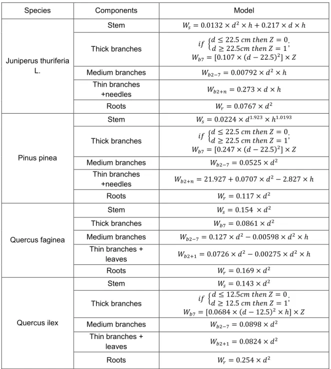
Biomass in the different components of the tree e.g., stem and branches (thick, medium and thin+needles) and roots were calculated from dbh and height using existing relative allometric equations (Table 1) developed by (Ruiz-Peinado Gertrudix, Montero, & del Rio, 2012; Ruiz-Peinado, del Rio, & Montero, 2011). Tree component biomass values were computed for individual tree within each quadrat, and summed up to derive a summary of tree biomass for each quadrat. Total biomass obtained from sum of the biomass of all components.
Table 1. Biomass allometric equations by species
Species Components Model
Juniperus thuriferia L.
Stem 𝑊𝑠= 0.0132 × 𝑑2× ℎ + 0.217 × 𝑑 × ℎ
Thick branches 𝑖𝑓 {𝑑 ≤ 22.5 𝑐𝑚 𝑡ℎ𝑒𝑛 𝑍 = 0𝑑 ≥ 22.5𝑐𝑚 𝑡ℎ𝑒𝑛 𝑍 = 1;
𝑊𝑏7= [0.107 × (𝑑 − 22.5)2] × 𝑍 Medium branches 𝑊𝑏2−7= 0.00792 × 𝑑2× ℎ
Thin branches
+needles 𝑊𝑏2+𝑛= 0.273 × 𝑑 × ℎ Roots 𝑊𝑟= 0.0767 × 𝑑2
Pinus pinea
Stem 𝑊𝑠= 0.0224 × 𝑑1.923× ℎ1.0193
Thick branches 𝑖𝑓 {𝑑 ≤ 22.5 𝑐𝑚 𝑡ℎ𝑒𝑛 𝑍 = 0𝑑 ≥ 22.5 𝑐𝑚 𝑡ℎ𝑒𝑛 𝑍 = 1;
𝑊𝑏7= [0.247 × (𝑑 − 22.5)2] × 𝑍 Medium branches 𝑊𝑏2−7= 0.0525 × 𝑑2
Thin branches
+needles 𝑊𝑏2+𝑛= 21.927 + 0.0707 × 𝑑2− 2.827 × ℎ
Roots 𝑊𝑟= 0.117 × 𝑑2
Quercus faginea
Stem 𝑊𝑠= 0.154 × 𝑑2
Thick branches 𝑊𝑏7= 0.0861 × 𝑑2
Medium branches 𝑊𝑏2−7= 0.127 × 𝑑2− 0.00598 × 𝑑2× ℎ Thin branches +
leaves 𝑊𝑏2+1= 0.0726 × 𝑑2− 0.00275 × 𝑑2× ℎ
Roots 𝑊𝑟= 0.169 × 𝑑2
Quercus ilex
Stem 𝑊𝑠= 0.143 × 𝑑2
Thick branches 𝑖𝑓 {𝑑 ≤ 12.5𝑐𝑚 𝑡ℎ𝑒𝑛 𝑍 = 0𝑑 ≥ 12.5 𝑐𝑚 𝑡ℎ𝑒𝑛 𝑍 = 1;
𝑊𝑏7= [0.0684 × (𝑑 − 12.5)2× ℎ] × 𝑍 Medium branches 𝑊𝑏2−7= 0.0898 × 𝑑2
Thin branches +
leaves 𝑊𝑏2+1= 0.0824 × 𝑑2
Roots 𝑊𝑟= 0.254 × 𝑑2
3.3. Tree species diversity estimation
The diversity indices used in this study were classified into 3 categories (Table 2). The basic idea of a diversity index is to obtain a quantitative estimate of biological variability that can be used to compare biological entities, composed of discrete components, in space or in time (Morris et al., 2014).
Table 2. Categorization of indices
Richness & diversity Species composition Distribution pattern Vertical Horizontal Simpson index (Sm) Mingling (Mi) Vertical Profile
index (A)
Aggregation index (R) Shannon index (Sn) Spatial Diversity Status
(MS) Height Differentiation index (TH) Uniform Angle Index (W Evenness index (E) Segregation index (S)
Berker-Parker index (D)
3.3.1. Species richness indices
Two different aspects are generally used to conceptualize the diversity in a community: species richness and evenness. Species richness represents the number of species or attributes present in a community which is the simplest and most commonly applied metric. The distribution of individuals over species is called evenness. Additionally, species or trait abundance is also important for diversity, and the proportional abundance of species can be incorporated into indices that represent diversity.
3.3.1.1. Simpson Diversity index (1-D)
The Simpson diversity index (Eq. 1) was introduced by Edward H. Simpson (Simpson, 1949) to measure species diversity in a community by taking into account the number of species present and the abundance of each species. The index represents the probability that two individuals that are randomly selected from a sample will belong to different species.
1 − 𝐷 = 1 −∑𝑅𝑖=1𝑛𝑖(𝑛𝑖 − 1) 𝑁(𝑁 − 1)
Eq. 1
where 𝑛𝑖 is the number of individuals belonging to 𝑖-th type, N is total number of individuals in the dataset, R– richness ( total number of species types in dataset).
It ranges 0 ≤ D ≤ 1. The value increases with species diversity. The higher the diversity, the greater the value of D.
3.3.1.2. Shannon index
Shannon index (𝐻℩) by Shannon and Weaver (Shannon, 1948) is distance independent index to characterize the species diversity in a given stand. It takes into account both abundance and evenness of the existing species (Eq. 2).
𝐻℩ = − ∑ 𝑝 𝑖ln 𝑝𝑖 𝑆
𝑖=1
Eq. 2
ranges from 0 to ln (S). When all species in the dataset are equally common, all pi values equal 1/S, and the Shannon index hence takes the value In(S). When all abundance is concentrated in one species, and the other species are very rare (even if there are many of them), its value reduces to 0. The value is 0 when only one species in the dataset. 3.3.1.3. Berker-Parker index (D)
Berker-Parker index (Berger & Parker, 1970) is a measure of the numerical importance of the most abundant species in the population (Eq. 3). It has an analytical relationship with the geometric series of the species abundance model and represents the proportional abundance of only the most abundant species in the population (Morris et al., 2014).
𝐷 =𝑁𝑚𝑎𝑥 𝑁
Eq. 3
where 𝑁𝑚𝑎𝑥 is the number of individuals is in the most abundant species and N is the total number of individuals in the sample. The reciprocal of the index, 1/D, is often used, so that an increase in the value of the index corresponds an increase in diversity and a reduction in dominance.
3.3.1.4. Evenness index (E)
Species evenness (E) (Pielou, 1975) refers to how species are close to each other in numbers (del Río et al., 2018). It represents the degree to which individuals disturb closely among species in terms of number. E is not calculated independently, but rather derived from compound diversity measures such as , D indices, as they inherently contain richness and evenness components. In Eq. 3, 𝐻℩ is the number derived from the Shannon diversity index and 𝐻℩𝑚𝑎𝑥 is the maximum possible value of 𝐻℩ (if every species was equally likely). E is supposed to be independent of a measure of species richness.
𝐸 =ln 𝑆𝐻℩ Eq. 4 where 𝐻℩ is a value of Shannon diversity index, lnS is natural logarithm of the number of species which equals to 𝐻℩𝑚𝑎𝑥. Its value falls between 0 and 1 (1 demonstrates complete evenness). Low values indicate that one or a few species dominate, and high values indicate that relatively equal numbers of individuals belong to each species. 3.3.2. Species intermingling
The spatial relationships between two groups of individuals play important role for many components of a species’ population biology. A numerous different types of tests indices have been designed to seek for an answer to the question whether two species are spatially segregated (individuals occur near the same species), associated (individuals occur near the other species), or neither.
3.3.2.1. Species segregation (S) index
trees i to every tree in the plot which derived from Euclidean distance calculation. Once the distances were computed, trees were ranked from nearest to farthest to reference tree and the first n-th number of neighboring trees (which are user dependent) were selected, 2) computation of S index: which was computed based on the nearest-neighbor tree distances calculated in 1st step. S is originally designed for being applied to a two-species mixture (Biber & Weyerhaeuser, 1998). In Pielou’s approach, a contingency table is constructed in form described in Table 3.
𝑆 = 1 −𝐸(𝑝𝑝𝑖𝑗
𝑖𝑗) = 1 −
𝑂𝑏𝑠𝑒𝑟𝑣𝑒𝑑 𝑛𝑢𝑚𝑏𝑒𝑟 𝑜𝑓 𝑚𝑖𝑥𝑒𝑑 𝑝𝑎𝑖𝑟𝑠 𝐸𝑥𝑝𝑒𝑐𝑡𝑒𝑑 𝑛𝑢𝑚𝑏𝑒𝑟 𝑜𝑓 𝑚𝑖𝑥𝑒𝑑 𝑝𝑎𝑖𝑟𝑠
Eq. 5
Pijand E(pij) can be solved by Eq. 6:
𝑆 = 1 −𝑁 ∗ (𝑏 + 𝑐)𝑚𝑤 + 𝑛𝑣 Eq. 6
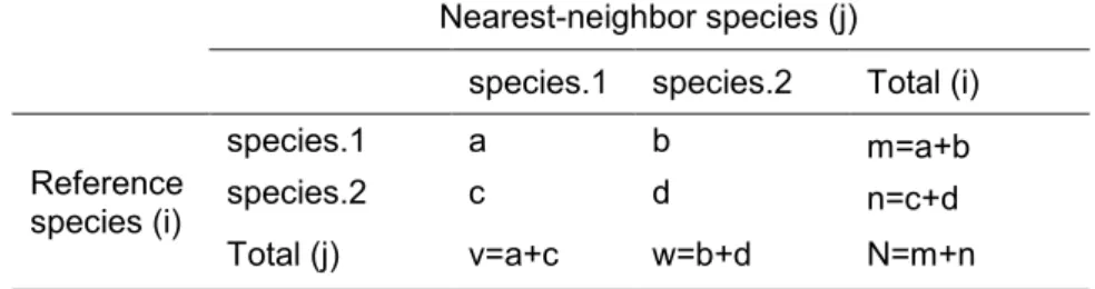
where: m and n are the observed number of individual trees of species 1 and 2 respectively. N can easily be extracted from sum of m and n as described in the table. The v and w are the number of individual trees of species 1 and 2 that are found as the nearest-neighbors of a reference tree. These variables are clearly described in a contingency table (Table 3).
Table 3. Descriptions of variables for S index calculation
Nearest-neighbor species (j)
species.1 species.2 Total (i)
Reference species (i)
species.1 a b m=a+b
species.2 c d n=c+d
Total (j) v=a+c w=b+d N=m+n
If the nearest-neighbors are always the same species as the reference trees, then S=1 which implies that the reference tree is associated with itself. There is a segregation of reference species from others. If all neighbors are different species, S=-1 which indicates that the reference tree is associated with other species. There is association between 2 species. Independent distribution of species is indicated by value near to 0.
𝑆 = {1, 𝑎𝑙𝑙 𝑛𝑒𝑎𝑟𝑒𝑠𝑡 𝑛𝑒𝑖𝑔ℎ𝑏𝑜𝑟𝑠 −1, 𝑎𝑙𝑙 𝑛𝑒𝑎𝑟𝑒𝑠𝑡 𝑛𝑒𝑖𝑔ℎ𝑏𝑜𝑟𝑠 𝑎𝑟𝑒 𝑡ℎ𝑒 𝑑𝑖𝑓𝑓𝑒𝑟𝑒𝑛𝑡 𝑡ℎ𝑎𝑛 𝑟𝑒𝑓𝑒𝑟𝑒𝑛𝑐𝑒 𝑡𝑟𝑒𝑒 (𝑖) 1 ≥ 𝑆 ≥ −1(𝑗) 𝑎𝑟𝑒 𝑡ℎ𝑒 𝑠𝑎𝑚𝑒 𝑠𝑝𝑒𝑐𝑖𝑒𝑠 𝑤𝑖𝑡ℎ 𝑟𝑒𝑓𝑒𝑟𝑒𝑛𝑐𝑒 𝑡𝑟𝑒𝑒 (𝑖)
3.3.2.2. Mingling (Mi) index
Species spatial mingling (Mi) index is a measure of species diversity within a structure unit (neighbor trees plus reference tree) which describes the proportion of neighbor trees which don’t belong to same species as the reference tree. The Mi by Füldner (1995) is defined as in Eq. 7 :
𝑀𝑖 =1𝑛 ∑ 𝑉𝑖𝑗 𝑛
𝑖
Eq. 7
𝑉𝑖𝑗 = {1, 𝑛𝑒𝑖𝑔ℎ𝑏𝑜𝑢𝑟(𝑗) 𝑏𝑒𝑙𝑜𝑛𝑔 𝑡𝑜 𝑑𝑖𝑓𝑓𝑒𝑟𝑒𝑛𝑡 𝑠𝑝𝑒𝑐𝑖𝑒𝑠 𝑓𝑟𝑜𝑚 𝑟𝑒𝑓𝑒𝑟𝑒𝑛𝑐𝑒 𝑡𝑟𝑒𝑒 (𝑖) 0 ≤ 𝑀0, 𝑛𝑒𝑖𝑔ℎ𝑏𝑜𝑢𝑟(𝑗) 𝑏𝑒𝑙𝑜𝑛𝑔 𝑡𝑜 𝑡ℎ𝑒 𝑠𝑎𝑚𝑝𝑒 𝑠𝑝𝑒𝑐𝑖𝑒𝑠 𝑎𝑠 𝑟𝑒𝑓𝑒𝑟𝑒𝑛𝑐𝑒 𝑡𝑟𝑒𝑒 (𝑖) 𝑖≤ 1
A low degree of mingling indicates that trees of a particular species occur together with few or no trees of different species in the same area. High degree of mingling means that trees are surrounded by different species. Assume there are 4 neighbor trees to a reference tree, 5 different outputs are possible to derive as shown in Figure 3. The distribution of the Mi values, in conjunction with the species proportions within a given tree population, allows a detailed study of the spatial diversity within a forest. However, the number of different species in the structure unit was not taken into account, and this was a shortcoming of the Mi index. This shortcoming has fulfilled in spatial diversity status index.
3.3.2.3. Spatial diversity status (MS)
𝑀𝑆𝑖 is improvement of mingling index. It considers not only the spatial mingling, but also the number of tree species. 𝑀𝑆𝑖 is determined by the relative species richness within the structure unit i and the degree of mingling of the reference tree and expressed by Eq. 8 (Gadow & Hui, 2002). The structural unit is defined by the neighborhoods that consisting a reference tree and its nearest neighbors (Zhang et al., 2018).
𝑀𝑆𝑖=𝑛𝑆𝑖 𝑚𝑎𝑥× 𝑀𝑖
Eq. 8. Where 𝑆𝑖 is the number of tree species in the neighborhood of the reference tree 𝑖, including tree 𝑖, and 𝑛𝑚𝑎𝑥 is the maximum number of species in this structure unit. 𝑀𝑖 is the species mingling value. MS measures the tree species richness as well as an important species characteristic within a structure unit. Reference tree of a common species is more likely to have the neighbors of the same species, reflecting low MS value. R rare species have less probability to have same neighbor species, resulting in high value of MS. Thus, MS is considered as an index that sensitive to rare species.
Mi
i
nd
ex 𝑀
𝑖= 0 4⁄ = 0 𝑀= 0.25𝑖= 1 4⁄ 𝑀𝑖= 2 4⁄ = 0.5 𝑀𝑖= 3 4⁄ = 0.75 𝑀𝑖= 04 4⁄ = 1
None of the neighbor tree is
different species than reference tree
One of the neighbor tree is
different species than reference tree
Two of the neighbor tree
are different species than reference tree
Three of the neighbor trees
are different species than reference tree
All 4 neighbor trees are
different species than reference tree
No mixture Low mixture Medium mixture High mixture Complete mixture
MS
i
nd
ex
𝑆𝑖⁄𝑛𝑚𝑎𝑥 = 1/4 𝑆𝑖 = 2/4 𝑆𝑖 = 2/4 𝑆𝑖 = 4/4 𝑆𝑖 = 4/4
Ther is 1 species (𝑎) in
the structure unit/max number of species in this structure unit is
4.
There are 2 species (𝑎, 𝑏) in the structure
unit/ max number of species in this structure unit is
4.
There are 2 species (𝑎, 𝑏) in
the structure unit/ max number of species in this structure unit is
4.
There are 4 species
(𝑎, 𝑏, 𝑐, 𝑑) in the structure unit/ max number of
species in this structure unit is
4.
There are 4 species
(𝑎, 𝑏, 𝑐, 𝑑) in the structure unit/ max number of
species in this structure unit is
4.
W
i
ndex 𝑊𝑖= 0 4⁄ = 0 𝑊𝑖= 1 4⁄
= 0.25 𝑊𝑖= 2 4⁄ = 0.5 𝑊𝑖= 3 4⁄ = 0.75 𝑊𝑖= 04 4⁄ = 1 None of the
angles (𝜃) is smaller than standard angle
(𝜃𝑠)
One of the angles (𝜃) is smaller than standard angle
(𝜃𝑠)
Two of the angles (𝜃) are
smaller than standard angle
(𝜃𝑠)
Three of the angles (𝜃) are
smaller than standard angle
(𝜃𝑠)
All of the angles (𝜃) is smaller than standard angle
(𝜃𝑠) Very regular Regular Random Clumped Very clumped
Figure 3.Description and calculation of Mingling index (Mi), Spatial diversity status (MS) and Uniform Angle index (Wi) and corresponding likelihood values for structure unit of 4 neighbors around the reference i tree: a, b, c, d are the tree species types ; 𝜽 are angles between adjacent neighbor trees; 𝜽𝒔 is a standard angle (which is equal to 360/4 for 4
neighbor trees) (Adapted from Gadow & Hui, 2002)
3.3.3. Spatial structural indices
vertical or horizontal axis (del Río et al., 2018). The horizontal spatial distribution gives an idea of the variation of tree positioning (Bravo & Guerra, 2002). The indices that measure the horizontal spatial distribution quantifies the degree of regularity of the trees which are typically classified into regular, random, and clustered patterns and linked to processes of tree mortality, competitive interaction, regeneration and gap creation and so on. Vertical spatial distribution is most commonly described in terms of layers that refer to distinct classes or stratification of the canopy corresponding to height-related differentiation between trees.
3.3.3.1. Uniform Angle Index (W)
The Uniform Angle Index (W) formulates the degree of spatial dispersion of nearest neighbors around the reference tree based on angles between adjusting nearest neighbor trees defined as vectors from reference tree to each neighbors as shown in Figure 3 (Gadow et al., 1998). W is determined as the proportion of the angles that are smaller than the standard angle 𝛼0 (360/ 𝑛) and calculated as (Eq. 9):
𝑊𝑖=𝑛 ∑ 𝑣1 𝑗 where 𝑣𝑗= { 0, otherwise 1, 𝛼𝑗< 𝛼0 𝑛
𝑗=1
Eq. 9
where 𝑛 is number of nearest neighbours
0 ≤ W ≤ 1; If { 0.5 < 𝑊 < 0.6, 𝑟𝑎𝑛𝑑𝑜𝑚 𝑑𝑖𝑠𝑡𝑟𝑖𝑏𝑢𝑡𝑖𝑜𝑛𝑊 < 0.5, 𝑟𝑒𝑔𝑢𝑙𝑎𝑟 𝑡𝑟𝑒𝑒 𝑑𝑖𝑠𝑡𝑟𝑖𝑏𝑢𝑡𝑜𝑖𝑛 𝑊 > 0.6, 𝑐𝑙𝑢𝑚𝑝𝑒𝑑
The value of W ranges from 0 to 1. The value of W increases from regular to clumped pattern (regular < random < clumped).
3.3.3.2. Aggregation index R
Aggregation index (R) by Clark & Evans (1954) is a single value index that is designed to describe aspects of variability of tree locations in forest stands (Eq. 10).
𝑅 =𝑟̅𝑜𝑏𝑠𝑒𝑟𝑣𝑒𝑑
𝐸(𝑟) where 𝐸(𝑟) = √ 𝐴 𝑁
Eq. 10
Where 𝑟̅𝑜𝑏𝑠𝑒𝑟𝑣𝑒𝑑 is an average distance to their nearest neighbours in a given forest stand while E(r) is an average nearest neighbor distance when trees completely random distributed, A is area of the plot, N is the total number of trees in the plot. The edge effect arising from the spatial limitations of experiment plots has minimized by applying the boundary correction factor by Donnelly (1978). Interpretation of R values is as follows:
0 ≤ 𝑅 ≤ 2.149: 𝑅 {< 1; 𝑡ℎ𝑒𝑛 𝑝𝑎𝑡𝑡𝑒𝑟𝑛 𝑠ℎ𝑜𝑤𝑠 𝑐𝑙𝑢𝑠𝑡𝑒𝑟𝑖𝑛𝑔 ≈ 1; 𝑡ℎ𝑒𝑛 𝑝𝑎𝑡𝑡𝑒𝑟𝑛 𝑖𝑠 𝑟𝑎𝑛𝑑𝑜𝑚 𝑑𝑖𝑠𝑡𝑟𝑖𝑏𝑢𝑡𝑖𝑜𝑛 > 1; 𝑡ℎ𝑒𝑛 𝑝𝑎𝑡𝑡𝑒𝑟𝑛 𝑖𝑠 𝑟𝑒𝑔𝑢𝑙𝑎𝑟 𝑑𝑖𝑠𝑡𝑟𝑖𝑏𝑢𝑡𝑖𝑜𝑛
3.3.3.3. Height Differentiation index (TH)
𝑇𝐻𝑖𝑗= 1 −𝑀𝐴𝑋(𝐻𝑀𝐼𝑁(𝐻𝑖, 𝐻𝑗) 𝑖, 𝐻𝑗)
Eq. 11
where 𝐻𝑖, & 𝐻𝑗 are the height of reference tree and neighbor tree respectively. 0 ≤ TH ≤ 1. If {𝑇𝐻 = 1, 𝑛𝑒𝑖𝑔ℎ𝑏𝑜𝑢𝑟 𝑡𝑟𝑒𝑒𝑠 ℎ𝑎𝑣𝑒 ℎ𝑖𝑔ℎ 𝑑𝑖𝑓𝑓𝑒𝑟𝑒𝑛𝑡𝑖𝑎𝑡𝑖𝑜𝑛 𝑖𝑛 ℎ𝑒𝑖𝑔ℎ𝑡𝑇𝐻 = 0, 𝑛𝑒𝑖𝑔ℎ𝑡𝑏𝑜𝑢𝑟 𝑡𝑟𝑒𝑒𝑠 ℎ𝑎𝑣𝑒 𝑒𝑞𝑢𝑎𝑙 ℎ𝑒𝑖𝑔ℎ𝑡
3.3.3.4. Vertical species profile (A)
Vertical species profile (A) (Pretzsch, 1995) is outlined in Eq. 12. Calculation is based on the Shannon and Weaver (Shannon, 1948) diversity index. A considers both proportion of the species within a stand and the presence of each species in different height zones (Eq. 12). Height zones were determined as a same way as Pretzsch (2009).
𝐴 = − ∑ ∑ 𝑝𝑖𝑗× ln(𝑝𝑖𝑗) 𝑍
𝑖=1 𝑆
𝑖=1
Eq. 12
where S represents the number of species present, Z is the number of height zones (three in this case), 𝑝𝑖𝑗 is the proportion of a species in the height zone 𝑝𝑖𝑗=𝑛𝑖𝑗
𝑁, N is the total number of individuals, 𝑛𝑖𝑗 is the number of individuals of the species i in the zone j. Standardization of A can be done by dividing A value by the maximum value of the A index, i.e. 𝐴𝑚𝑎𝑥 = 𝑙𝑛(𝑆 × 𝑍). Its value is greater than 0. For a pure stand with single layer, A equals to 0. Its value is increases as heterogeneous the vertical profile increases.
3.4. Statistical analysis
We used multiple linear regressions to evaluate the relationship between tree biomass and diversity indices in the stand, where total biomass (B) per tree was the dependent variable, and species richness, composition and species distribution indices were covariates of interest. Following previous researches that have developed a various regression models for estimating total-tree and tree compartment biomass, we utilized following three general forms of linear and non-linear regression equations (Eq. 13 to Eq. 15) for development of different forms of prediction models.
𝑌 = 𝛽0+ 𝛽1𝑥1+ ⋯ + 𝛽𝑘𝑥𝑗+ 𝜀 Eq. 13 𝑌 = 𝛽0𝑥1𝛽1𝑥2𝛽2… 𝑥𝑗𝛽𝑘+ 𝜀 Eq. 14
𝑌 = 𝛽0𝜋(𝑥𝑖𝑥𝑗)𝛽𝑘
Eq. 15
ln 𝑌 = ln 𝛽0+ 𝛽1ln 𝑥𝑖+ ⋯ 𝛽2ln 𝑥𝑗 + 𝜀 Eq. 16 ln 𝑌 = ln 𝛽0+ 𝛽1ln(𝑥𝑖∗ 𝑥𝑗) + 𝜀 Eq. 17 where ln is the natural logarithm. 𝜀 is the random error term which is assumed to be normally distributed with mean zero and variance constant.
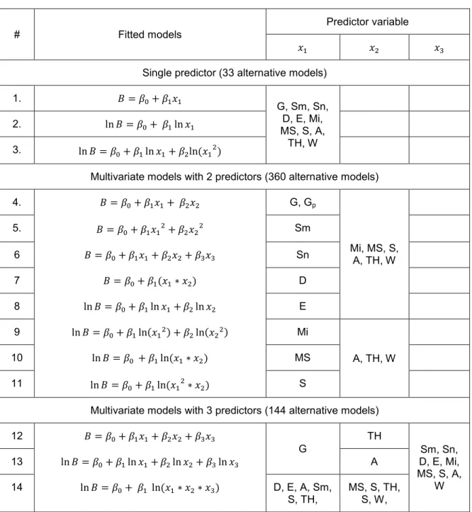
The models structures and their corresponding predictor variables are given in Table 4. 11 predictor variables: four species richness indices (Sm, Sn, D, E), three species composition indices (Mi, MS, S), four spatial distribution indices: A, TH, W and G were used as predictor variables for fitting models. Several different ways were implemented in variable selection process for the fitting models in order to avoid a problem of collinearity. First, all the variables were used as a single predictor variable for the models with single term. Second, basal area, species richness indices and species composition indices were utilized as state variables individually and each one of the spatial distribution indices were added into the multivariable models with two terms as secondary predictor variable. Third, we tested G, TH or A as a second, other individual indices as a third predictor variable for the multivariable models with three terms. Finally all possible combinations of indices are examined for multivariable models as well. In total, 537 alternative models were examined for each individual species and community level. For the community level analyze, basal area per quadrant G (m2/ha), for the species level analyze, species proportion of basal area 𝐺𝑝 per quadrant were explored.
Table 4. Fitting models and their predictor variable reference
# Fitted models
Predictor variable
𝑥1 𝑥2 𝑥3
Single predictor (33 alternative models)
1. 𝐵 = 𝛽0+ 𝛽1𝑥1
G, Sm, Sn, D, E, Mi, MS, S, A,
TH, W 2. ln 𝐵 = 𝛽0+ 𝛽1ln 𝑥1
3. ln 𝐵 = 𝛽0+ 𝛽1ln 𝑥1+ 𝛽2ln(𝑥12)
Multivariate models with 2 predictors (360 alternative models)
4. 𝐵 = 𝛽0+ 𝛽1𝑥1+ 𝛽2𝑥2 G, Gp
Mi, MS, S, A, TH, W
5. 𝐵 = 𝛽0+ 𝛽1𝑥12+ 𝛽2𝑥22 Sm
6 𝐵 = 𝛽0+ 𝛽1𝑥1+ 𝛽2𝑥2+ 𝛽3𝑥3 Sn
7 𝐵 = 𝛽0+ 𝛽1(𝑥1∗ 𝑥2) D
8 ln 𝐵 = 𝛽0+ 𝛽1ln 𝑥1+ 𝛽2ln 𝑥2 E 9 ln 𝐵 = 𝛽0+ 𝛽1ln(𝑥12) + 𝛽2ln(𝑥22) Mi
A, TH, W
10 ln 𝐵 = 𝛽0 + 𝛽1ln(𝑥1∗ 𝑥2) MS
11 ln 𝐵 = 𝛽0+ 𝛽1ln(𝑥12∗ 𝑥2) S
Multivariate models with 3 predictors (144 alternative models)
12 𝐵 = 𝛽0+ 𝛽1𝑥1+ 𝛽2𝑥2+ 𝛽3𝑥3
G
TH
Sm, Sn, D, E, Mi, MS, S, A,
W 13 ln 𝐵 = 𝛽0+ 𝛽1ln 𝑥1+ 𝛽2ln 𝑥2+ 𝛽3ln 𝑥3 A
14 ln 𝐵 = 𝛽0+ 𝛽1 ln(𝑥1∗ 𝑥2∗ 𝑥3) D, E, A, Sm, S, TH,
MS, S, TH, S, W,
4. - RESULTS
From the result of 537 investigated models, 11 significant models for community level are summarized in Table 5. Parameters of all models were statistically significant at (𝑝 < 0.01). TH alone or in combination with species richness or composition indices i.e Sm+TH, Sm*TH, Sn*TH, D+TH, E+TH, E*TH, Mi+TH, MS+TH, S+TH, G+TH+Sm, G+TH+MS was a main explanatory variable in all models except model 10 demonstrating the importance of vertical structural on tree biomass. According to parameter estimation, negative parameters were associated to species richness and compositional indices (Sm in model 1 and 4; MS in model 2 and 10; Mi in model 9; S in model 11 in logarithmic form) while positive parameters were correspond to TH in all the models excluding models 5 and 8 which implies that biomass increases as species richness or species composition decreases and height heterogeneity increases. From the selected 11 models, model 6 (Eq. 18) was found to be the best model for predicting community level tree biomass, showing negatively influence of D and positively influence of TH on tree biomass of the stand.
Ln 𝐵 = 6.594 − 1.349 ln 𝐷 + 0.841 ln 𝑇𝐻 Eq. 18
Where B is total biomass per tree (kg), D is Berker-Parker index, TH is height differentiation index.
Table 6 showed that the parameter estimates of selected models by species based on models in Table 4. Similar trend that had observed at community level occur
for Pinus pinea: TH alone or in combination with species richness or composition indices
such as Sm+TH; Sm*TH; Sn+TH; Sn*TH; D+TH; D*TH; E*TH, Mi*TH was a main explanatory variable for all the models. The strength of the relationship ranges from 0.02 to 0.16 (0.16 < R2 < 0.2). The highest statistically significant and the lowest AIC value belong to Eq. 19 (model 6, Table 6). The same form of model as community level analysis has been chosen as a best model for Pinus pinea as well. The reciprocal interactive effect of D and TH had the best prediction power on biomass. 𝐺𝑝 has been shown to be the best explanatory variable for the biomass for both Quercus faginea (Eq. 20) and Quercus ilex (Eq. 21). None of the model was significant for Juniperus thurifera
as concerned by models in this study.
ln 𝐵 = 7.249 − 0.935 ln 𝐷 + 0.988 ln 𝑇𝐻 Eq. 19
ln 𝐵 = 4.278 + 0.156 ln 𝐺𝑝 Eq. 20
Intercept logG logD logTH logSm logMS log(Sm*TH) logE logMi logS log(E*TH) 1 2.929*** (0.638) 0.812*** (0.217) 0.763*** (0.098) -11.142***
(2.953) 437 0.20 1264.2 1.02 37.809*** 2 4.426***
(0.594) 0.706*** (0.213) 0.990*** (0.097) -2.028***
(0.465) 437 0.21 1259.6 1.02 39.746*** 3 5.684***
(0.137)
0.883***
(0.096) 437 0.16 1283.9 1.05 84.958***
4 5.191*** (0.207)
0.797*** (0.099)
-9.264***
(2.954) 437 0.18 1276.1 1.04 48.260*** 5 5.717***
(0.142)
0.881***
(0.097) 437 0.16 1285.8 1.05 82.659*** 6 6.594***
(0.218)
-1.349*** (0.257)
0.841***
(0.093) 437 0.21 1258.9 1.02 58.877***
7 6.149*** (0.185)
0.894*** (0.095)
32.906***
(8.965) 437 0.19 1272.5 1.03 50.434*** 8 5.701***
(0.138) 0.887*** (0.096) 437 0.16 1283.2 1.05 85.791*** 9 6.466***
(0.217)
1.038*** (0.100)
-1.319***
(0.288) 437 0.20 1265.2 1.02 54.926*** 10 6.288***
(0.197)
1.001*** (0.098)
-1.973***
(0.470) 437 0.19 1268.5 1.03 52.898*** 11 5.963***
(0.146)
0.710*** (0.101)
-2.125***
(0.452) 437 0.20 1264.2 1.02 55.575***
***p<0.01
F.value Model
Explainatory variable
Table 6. Parameter estimates for biomass from selected models at species level
Intercept logTH logSm log(Sm*TH) logSn log(Sn*TH) logD log(D*TH) log(E*TH) log(Mi*TH+1) logG log(E+1) log(E+1)^2 log(D+1) log(D+1)^2
1 6.575***
(0.191)
0.937***
(0.163) 177 0.16 488.5 0.95 33.191***
2 6.158***
(0.249)
0.926*** (0.160)
-8.738**
(3.391) 177 0.18 483.8 0.94 20.452***
3 6.596***
(0.199)
0.917***
(0.163) 177 0.15 489.9 0.96 31.494***
4 7.986***
(0.662)
0.923*** (0.161)
-1.230**
(0.553) 177 0.17 485.5 0.94 19.444***
5 5.500***
(0.074)
0.774***
(0.162) 177 0.11 497.5 0.98 22.873***
6 7.249***
(0.289)
0.988*** (0.160)
-0.935***
(0.306) 177 0.19 481.2 0.93 22.060***
7 5.782***
(0.098)
0.532***
(0.145) 177 0.07 506.2 1.00 13.398***
8 6.594***
(0.193)
0.943***
(0.163) 177 0.16 488.1 0.95 33.613***
9 5.004***
(0.129)
2.864***
(0.556) 177 0.13 494.3 0.97 26.489***
1 4.278***
(0.170)
0.156**
(0.072) 157 0.023 183.2 0.43 4.632**
1 4.241***
(0.126)
0.168***
(0.045) 69 0.157 74.3 0.403 13.702***
**p < 0.05; ***p < 0.01 F.value
Pinus pinea
Quercus ilex Quercus faginea
the stand influenced negatively and height heterogeneity influenced positively on biomass at community level. For the species level analysis, the variation of biomass of
Pinus pinea can be explained by the same model as community level analysis which
highlighted the negative impact of D and the positive impact of TH on biomass. This results is agreement with Bohn & Huth, (2017) who examined an influence of species diversity and forest structure on aboveground biomass over a broad range of forest stands and found out a positive relation between forest structural diversity and forest productivity. The same result was found in Riofrío et al., (2017). Size heterogeneity enables bigger trees to obtain greater amount of a certain resource and use them more efficiently than small trees (Brockerhoff et al., 2017b). In our stand, mixture of the Pine, Quercus faginea, Quercus ilex and Juniperus thurifera might create a different canopy strata; top layer occupied by Pinus pinea, enabling the light-demanding species – Pine -
to capture more light and grow better than other species and become dominant in the stand.
The variation of biomass for Quercus faginea and Quercus ilex were predicted by basal area proportion of species (Gp). The examined diversity indices such as Sm, Sn, D, E, Mi, MS, S, W, A, TH were found not significant relation with biomass of Quercus. This might be explained by abundance of Pinus pinea. The abundance of Pine have an strong inhibitory effect on the abundance and richness of understory species through light, water, and soil nutrients and thus reversely influences on biomass productivity of understory species (Laughlin & Grace, 2006). Moreover, biomass of individual tree in a given stand is not only the reflection of diversity (species richness, composition and structure) but also various internal and external factors such as age, stand density, site productivity, competition at the tree level, climate, soil (texture, moisture content), geographical location, and length of grown season (Con et al., 2013; Poudel & Hailemariam, 2015) which might not be reflected by the available metrics or models that we are considered in this study.
One notable thing is that almost all the predictor variables of significant models (except model 1 in Table 6) for Pinus pinea were identical with the community level models in Table 5. This might be fact that community level analysis may be influenced by characteristic of Pinus pinea due to its dominance in the stand. This can be explained by “selection effect” which describes the impact of the most productive species on relationship between species richness and productivity. Positive relation between productivity (biomass accumulation) and tree diversity largely depends on presenting highly productivity species in multi-cultural communities (Tilman, 1999). However, in our case the proportion of the most productive, dominant species (Pinus pinea) showed a negative effect on biomass stand as represented by D in Eq. 18 & Eq. 19. As stress-tolerant and pioneer species, Pinus has the ability to become a dominant tree species in the mixed forest and accumulate biomass in a short time and it is considered as a strong competitor species with relatively high production due to its prolonged photosynthetic activity (coniferous evergreen tree) and high nutrient uptake through the rapid turnover of nutrients (Li, Su, Lang, Liu, & Ou, 2018). In old growth stand, Pinus with large diameter have a greater contribution to the stand biomass than small diameter trees (Baishya & Barik, 2011). In terms of complementarity of the species in this stand, Pinus
pinea may facilitate development of Quercus by increasing seed protections, enhancing
habitat condition which promote the recruitment of Quercus (Sheffer, 2012). Nevertheless, the facilitation of Pine for Quercus colonization depends on many factors such as stand density, development stage of Quercus, and environmental conditions.
Pine forests with intermediate density enhance the site conditions for successful
improving the soil moisture status for Quercus seedlings. However, there is an opposition between suitable condition for recruitment and suitable condition for further growth and development of Quercus species that after seedlings and saplings stages (Puerta-Piñero, Gómez, & Valladares, 2007). In dense forest with poor environmental condition, although Pinus improved soil properties during a short period (a decade), it causes in decrement of soil moisture which may reduce recruitment of Quercus in their subcanopy. Low light interception levels and competition for water with Pinus reduces
Quercus colonization in poor environmental condition. Maestre & Cortina, (2004)
emphasized that Pine plantation in semi-arid environment don’t facilitate the establishment of Quercus and causes in reduction of species richness and all plant cover. Therefore, based on these reviews, we can say that Pinus pinea might be a main contributor for biomass of the stand whereas its abundance has negatively impact on biomass of coexisting species i.e Quercus faginea, Quercus ilex and Juniperus thurifera.
6. - CONCLUSIONS
In this study, we examined the relationship between tree biomass and diversity in Llano de San Marugan, Valladolid, Spain at stand and individual species level by a various linear and non-linear models. After thoughtful examination of 537 models with 11 predictor tree diversity indices, we found out that there is a relation between tree biomass and diversity although this relation varies among the species. A stand level analyze revealed that tree biomass-diversity relation can be explained by an interaction of negative affect of abundance of dominant species and positive effect of tree’ height heterogeneity which indicates that tree biomass increases as abundance of dominant species decreases and height heterogeneity increases. This result was identical for
Pinus pinea. For Quercus faginea and Quercus ilex, only the species proportion of basal
7. - AKNOWLEDGEMENTS
The author would like to greatly appreciate and acknowledge the following people for their help and support for success of this study:
- For supervisor Prof. Felipe Oviedo Bravo and co-supervisor Cristobal Ordonez Alonso for their enormous amount of contribution, guidance, critical comments, suggestion and helpful instructions from the initial to final stages which truly permits to successful completion of this work.
- For all the professors, staffs at University of Valladolid and University of Padova for sharing their valuable knowledge, skills and experiences which helped me a lot to strengthen my knowledge and experience in this science.
- For MEDfOR program for not only for the financial support but also letting us to build international network of friendship and living and experiencing in different countries with different culture.
8. - REFERENCES
Baishya, R., & Barik, S. K. (2011). Estimation of tree biomass, carbon pool and net primary production of an old-growth Pinus kesiya Royle ex. Gordon forest in north-eastern India. Annals of Forest Science, 68(4), 727–736. https://doi.org/10.1007/s13595-011-0089-8
Baskin, Y. (1994). Ecologists Dare to Ask: How Much Does Diversity Matter? Science,
264(5156), 202–203. https://doi.org/10.1126/SCIENCE.264.5156.202
Berger, W. H., & Parker, F. L. (1970). Diversity of Planktonic Foraminifera in Deep-Sea
Sediments. Science, 168(3937), 1345–1347.
https://doi.org/10.1126/science.168.3937.1345
Biber, P., & Weyerhaeuser, H. (1998). Numerical methods for characterizing structure and diversity applied to a natural tropical forest and an even aged teak stand. …
and Socio-Economic Analysis …. Retrieved from
http://www.wwk.forst.tu-muenchen.de/info/publications/OnlinePublications/482.pdf
Bohn, F. J., & Huth, A. (2017). The importance of forest structure to biodiversity– productivity relationships. Royal Society Open Science, 4(1), 160521. https://doi.org/10.1098/rsos.160521
Bravo-Oviedo, Andres, Pretzsch, H., Ammer, C., Andenmatten, E., Barbati, A., Barreiro, S., … Zlatanov, T. (2014). European Mixed Forests: definition and research perspectives. Forest Systems, 23(3), 518. https://doi.org/10.5424/fs/2014233-06256 Bravo, F., & Guerra, B. (2002). Forest Structure and Diameter Growth in Maritime Pine in a Mediterranean Area (pp. 123–134). Springer, Dordrecht. https://doi.org/10.1007/978-94-015-9886-6_10
Brockerhoff, E. G., Barbaro, L., Castagneyrol, B., Forrester, D. I., Gardiner, B., González-Olabarria, J. R., … Jactel, H. (2017a). Forest biodiversity, ecosystem functioning and the provision of ecosystem services. Biodiversity and Conservation,
26(13), 3005–3035. https://doi.org/10.1007/s10531-017-1453-2
Brockerhoff, E. G., Barbaro, L., Castagneyrol, B., Forrester, D. I., Gardiner, B., González-Olabarria, J. R., … Jactel, H. (2017b). Forest biodiversity, ecosystem functioning and the provision of ecosystem services. Biodiversity and Conservation,
26(13), 3005–3035. https://doi.org/10.1007/s10531-017-1453-2
Cardinale, B. J., Wright, J. P., Cadotte, M. W., Carroll, I. T., Hector, A., Srivastava, D. S., … Weis, J. J. (2007). Impacts of plant diversity on biomass production increase through time because of species complementarity. Proceedings of the National
Academy of Sciences of the United States of America, 104(46), 18123–18128.
https://doi.org/10.1073/pnas.0709069104
Clark, P. J., & Evans, F. C. (1954). Distance to Nearest Neighbor as a Measure of Spatial Relationships in Populations. Ecology, 35(4), 445–453. https://doi.org/10.2307/1931034
Con, T. Van, Thang, N. T., Ha, D. T. T., Khiem, C. C., Quy, T. H., Lam, V. T., … Sato, T. (2013). Relationship between aboveground biomass and measures of structure and species diversity in tropical forests of Vietnam. Forest Ecology and Management,
310, 213–218. https://doi.org/10.1016/J.FORECO.2013.08.034
Daily, G. C. (1997). Nature’s services : societal dependence on natural ecosystems. Island Press.
Stocks (pp. 301–327). Springer, Cham. https://doi.org/10.1007/978-3-319-28250-3_15
del Río, M., Pretzsch, H., Alberdi, I., Bielak, K., Bravo, F., Brunner, A., … Bravo-Oviedo, A. (2018). Characterization of Mixed Forests BT - Dynamics, Silviculture and Management of Mixed Forests. In Andrés Bravo-Oviedo, H. Pretzsch, & M. del Río (Eds.) (pp. 27–71). Cham: Springer International Publishing. https://doi.org/10.1007/978-3-319-91953-9_2
Evans, E. W. (2016). Biodiversity, ecosystem functioning, and classical biological control. Applied Entomology and Zoology. Springer. https://doi.org/10.1007/s13355-016-0401-z
Fraser, L. H., Pither, J., Jentsch, A., Sternberg, M., Zobel, M., Askarizadeh, D., … Zupo, T. (2015). Plant ecology. Worldwide evidence of a unimodal relationship between productivity and plant species richness. Science (New York, N.Y.), 349(6245), 302– 305. https://doi.org/10.1126/science.aab3916
Füldner, K. (1995). Strukturbeschreibung von Buchen-Edellaubholz-Mischwäldern. PhD,
[Describing forest structures in mixed beech-ash-maple-sycamore stands.
University of Göttingen, Cuvillier Verlag Göttingen,.
Gadow, K.v., Hui, G.Y., Albert, M. (1998). Das Winkelmaß–ein Strukturparameter zur Beschreibung der Individualverteilung in Waldbesta¨nden [The uniform angle index—a structural parameter for describing tree distribution in forest stands].
Centralbl. Ges. Forstwesen, (115), 1–10.
Gadow, K.v. (1993). Zur Bestandesbeschreibung in der Forsteinrichtung. Forst Und Holz, 48, 601–606.
Gadow Kv; Hui GY. (2002). No Title. In Characterizing forest spatial structure and
diversity. Lund: Proceedings of the Sustainable Forestry in Southern Sweden
(SUFOR) conference “Sustainable Forestry in Temperate Regions”,.
Gamfeldt, L., Snäll, T., Bagchi, R., Jonsson, M., Gustafsson, L., Kjellander, P., … Bengtsson, J. (2013). Higher levels of multiple ecosystem services are found in forests with more tree species. Nature Communications, 4. https://doi.org/10.1038/ncomms2328
Grace, J. B., Anderson, T. M., Seabloom, E. W., Borer, E. T., Adler, P. B., Harpole, W. S., … Smith, M. D. (2016). Integrative modelling reveals mechanisms linking productivity and plant species richness. Nature, 529(7586), 390–393. https://doi.org/10.1038/nature16524
Hooper, D. U., Adair, E. C., Cardinale, B. J., Byrnes, J. E. K., Hungate, B. A., Matulich, K. L., … O’Connor, M. I. (2012). A global synthesis reveals biodiversity loss as a major driver of ecosystem change. Nature, 486(7401), 105–108. https://doi.org/10.1038/nature11118
Iranah, P., Lal, P., Wolde, B. T., & Burli, P. (2018). Valuing visitor access to forested areas and exploring willingness to pay for forest conservation and restoration finance: The case of small island developing state of Mauritius. Journal of
Environmental Management, 223, 868–877.
https://doi.org/10.1016/j.jenvman.2018.07.008
Knoke, T., Stimm, B., Ammer, C., & Moog, M. (2005). Mixed forests reconsidered: A forest economics contribution on an ecological concept. Forest Ecology and
Management, 213(1–3), 102–116. https://doi.org/10.1016/j.foreco.2005.03.043
Laughlin, D. C., & Grace, J. B. (2006). A multivariate model of plant species richness in forested systems: old-growth montane forests with a long history of fire. Oikos,
114(1), 60–70. https://doi.org/10.1111/j.0030-1299.2006.14424.x
Li, S., Su, J., Lang, X., Liu, W., & Ou, G. (2018). Positive relationship between species richness and aboveground biomass across forest strata in a primary Pinus kesiya forest. Scientific Reports, 8(1), 2227. https://doi.org/10.1038/s41598-018-20165-y Liang, J., Crowther, T. W., Picard, N., Wiser, S., Zhou, M., Alberti, G., … Reich, P. B.
(2016). Positive biodiversity-productivity relationship predominant in global forests.
Science, 354(6309), aaf8957–aaf8957. https://doi.org/10.1126/science.aaf8957
Liu, C. L. C., Kuchma, O., & Krutovsky, K. V. (2018). Mixed-species versus monocultures in plantation forestry: Development, benefits, ecosystem services and perspectives for the future. Global Ecology and Conservation, 15, e00419. https://doi.org/10.1016/J.GECCO.2018.E00419
Maestre, F. T., & Cortina, J. (2004). Are Pinus halepensis plantations useful as a restoration tool in semiarid Mediterranean areas? Forest Ecology and Management,
198(1–3), 303–317. https://doi.org/10.1016/J.FORECO.2004.05.040
Mori, A. S., Lertzman, K. P., & Gustafsson, L. (2017). REVIEW: FOREST BIODIVERSITY AND ECOSYSTEM SERVICES Biodiversity and ecosystem services in forest ecosystems: a research agenda for applied forest ecology.
Journal of Applied Ecology, 54, 12–27. https://doi.org/10.1111/1365-2664.12669
Morris, E. K., Caruso, T., Buscot, F., Fischer, M., Hancock, C., Maier, T. S., … Rillig, M. C. (2014). Choosing and using diversity indices: insights for ecological applications from the German Biodiversity Exploratories. Ecology and Evolution, 4(18), 3514– 3524. https://doi.org/10.1002/ece3.1155
Ozcelik, R. (2009). Tree species diversity of natural mixed stands in eastern Black sea and western Mediterranean region of Turkey. Journal of Environmental Biology,
30(5), 761–766.
Pielou, E. C. (1975). Ecological diversity. New York: Wiley.
Pielou, E. C. (1977). Mathematical ecology. New York: John Wiley & Sons, Ltd.
Poudel, K. P., & Hailemariam, T. (2015). METHODS FOR ESTIMATING ABOVEGROUND BIOMASS AND ITS COMPONENTS FOR FIVE PACIFIC
NORTHWEST TREE SPECIES. Retrieved from
https://www.fs.fed.us/pnw/pubs/pnw_gtr931/pnw_gtr931_004.pdf
Pretzsch, H. (2009). Forest Dynamics, Growth, and Yield. In Forest Dynamics, Growth and Yield: From Measurement to Model (pp. 1–39). Berlin, Heidelberg: Springer Berlin Heidelberg. https://doi.org/10.1007/978-3-540-88307-4_1
Pretzsch, H., & Schütze, G. (2014). Size-structure dynamics of mixed versus pure forest stands. Forest Systems, 23(3), 560. https://doi.org/10.5424/fs/2014233-06112 Pretzsch, & H. (1995). Zum Einfluss des Baumvertielungsmusters auf den
Bestandszuwachs. Allg Forst-Jagd, 166, 190–201. Retrieved from https://ci.nii.ac.jp/naid/10029731191/#cit
Puerta-Piñero, C., Gómez, J. M., & Valladares, F. (2007). Irradiance and oak seedling survival and growth in a heterogeneous environment. Forest Ecology and
Management, 242(2–3), 462–469. https://doi.org/10.1016/J.FORECO.2007.01.079
Riofrío, J., del Río, M., Pretzsch, H., & Bravo, F. (2017). Changes in structural heterogeneity and stand productivity by mixing Scots pine and Maritime pine.
Forest Ecology and Management, 405, 219–228.
Ruiz-Peinado Gertrudix, R., Montero, G., & del Rio, M. (2012). Biomass models to estimate carbon stocks for hardwood tree species. Forest Systems; Vol 21, No 1
(2012)DO - 10.5424/Fs/2112211-02193 . Retrieved from
http://revistas.inia.es/index.php/fs/article/view/2193
Ruiz-Peinado, R., del Rio, M., & Montero, G. (2011). New models for estimating the carbon sink capacity of Spanish softwood species. Forest Systems; Vol 20, No 1
(2011)DO - 10.5424/Fs/2011201-11643 . Retrieved from
http://revistas.inia.es/index.php/fs/article/view/1880
Sala, O. E., Chapin, F. S., Armesto, J. J., Berlow, E., Bloomfield, J., Dirzo, R., … Wall, D. H. (2000). Global biodiversity scenarios for the year 2100. Science (New York,
N.Y.), 287(5459), 1770–1774. Retrieved from
http://www.ncbi.nlm.nih.gov/pubmed/10710299
Scarascia-Mugnozza, G., Oswald, H., Piussi, P., & Radoglou, K. (2000). Forests of the Mediterranean region: gaps in knowledge and research needs. Forest Ecology and
Management, 132(1), 97–109. https://doi.org/10.1016/S0378-1127(00)00383-2
Shannon, C. E. (1948). A Mathematical Theory of Communication. Bell System
Technical Journal, 27(3), 379–423.
https://doi.org/10.1002/j.1538-7305.1948.tb01338.x
Sheffer, E. (2012). A review of the development of Mediterranean pine–oak ecosystems after land abandonment and afforestation: are they novel ecosystems? Annals of
Forest Science, 69(4), 429–443. https://doi.org/10.1007/s13595-011-0181-0
Simpson, E. H. (1949). Measurement of Diversity. Nature, 163(4148), 688–688. https://doi.org/10.1038/163688a0
Szwagrzyk, J., & Gazda, A. (2007). Above‐ground standing biomass and tree species diversity in natural stands of Central Europe. Journal of Vegetation Science, 18(4), 555–562. https://doi.org/10.1111/j.1654-1103.2007.tb02569.x
Tilman, D, Lehman, C. L., & Thomson, K. T. (1997). Plant diversity and ecosystem productivity: theoretical considerations. Proceedings of the National Academy of
Sciences of the United States of America, 94(5), 1857–1861.
https://doi.org/10.1073/pnas.94.5.1857
Tilman, David. (1999). THE ECOLOGICAL CONSEQUENCES OF CHANGES IN BIODIVERSITY: A SEARCH FOR GENERAL PRINCIPLES. Ecology, 80(5), 1455– 1474. https://doi.org/10.1890/0012-9658(1999)080[1455:TECOCI]2.0.CO;2
Wang, H., Zhang, G., Hui, G., Li, Y., Hu, Y., & Zhao, Z. (2016). The influence of sampling unit size and spatial arrangement patterns on neighborhood-based spatial structure analyses of forest stands. Forest Systems, 25(1). https://doi.org/10.5424/fs/2016251-07968
ANNEX
Annex 1. Descriptive statistics of stand variables (437 trees in the one hectare plot)
Variables Mean St.Dev Min Pctl(25) Pctl(75) Max
B 137.4 196.7 2.9 26.2 128.4 1.067.5
d 16.6 11.7 3.0 8.6 23.1 50.5
h 5.8 2.5 2.0 4.0 7.6 13.0
V 0.1 0.2 0.001 0.01 0.1 1.2
Gi (m2/ha) 14.3 3.1 8.8 12.5 16.8 19.4
Sm 1.0 0.02 0.9 1.0 1.0 1.0
Sn 3.3 0.4 2.4 3.2 3.5 3.9
E 1.0 0.01 1.0 1.0 1.0 1.0
D 2.1 0.4 1.2 1.9 2.3 2.6
Mi 0.6 0.3 0.0 0.5 0.8 1.0
MS 0.3 0.1 0.0 0.2 0.4 0.6
W 0.5 0.2 0.0 0.2 0.8 1.0
S 0.3 0.2 0.1 0.2 0.3 0.9
A 2.5 0.8 0.0 1.9 3.1 3.7
TH 0.3 0.1 0.0 0.2 0.4 0.7
B – total biomass (kg); d – breast height diameter (m); h – total height (m), V – volume (m3), Sm - simson index; Sn – shannon index; E – evenness index; G- basal area (m2/ha), D – barker Parker index, Mi – mingling index; MS – spatial diversity status; W –
# Species N d (cm) h (m) v (m3) g (m2) B (kg) Sm Sn D E Mi MS S W A TH
1 Pinus pinea 177 27.512 8.163 0.256 0.070 290.110 0.955 3.215 1.985 0.987 0.549 0.251 0.194 0.489 1.900 0.366
2 Quercus faginea 157 9.604 4.183 0.019 0.008 38.757 0.963 3.390 2.141 0.987 0.562 0.260 0.239 0.497 2.965 0.263
3 Quercus ilex 69 9.100 4.122 0.013 0.007 27.122 0.969 3.548 2.130 0.987 0.558 0.270 0.612 0.446 3.137 0.226
4 Juniperus thurifera 34 7.626 4.331 0.271 0.005 21.764 0.956 3.202 2.189 0.981 0.765 0.312 0.241 0.507 2.683 0.251