Identification of intermediate debonding damage in FRP-plated RC beams based on multi-objective particle swarm optimization without updated baseline model

Identification of intermediate debonding damage in FRP-plated RC

beams based on multi-objective particle swarm optimization without

updated baseline model

Ricardo Perera Enrique Sevillano Angel Arteaga Ana De Diego

A B S T R A C T

Fiber reinforced polymer composites (FRP) have found widespread usage in the repair and strengthening of concrete structures. FRP composites exhibit high strength-to-weight ratio, corrosion resistance, and are convenient to use in repair applications. Externally bonded FRP flexural strengthening of concrete beams is the most extended application of this technique. A common cause of failure in such members is associated with intermediate crack-induced debonding (IC debonding) of the FRP substrate from the concrete in an abrupt manner. Continuous monitoring of the concrete-FRP interface is essential to pre-vent IC debonding. Objective condition assessment and performance evaluation are challenging activities since they require some type of monitoring to track the response over a period of time. In this paper, a multi-objective model updating method integrated in the context of structural health monitoring is dem-onstrated as promising technology for the safety and reliability of this kind of strengthening technique. The proposed method, solved by a multi-objective extension of the particle swarm optimization method, is based on strain measurements under controlled loading. The use of permanently installed fiber Bragg grating (FBG) sensors embedded into the FRP-concrete interface or bonded onto the FRP strip together with the proposed methodology results in an automated method able to operate in an unsupervised mode.

1. Introduction

Nowadays, fiber reinforced polymers (FRP) have found wide-spread usage in civil structures, especially for the strengthening and rehabilitation of existing concrete structures [1-3]. High strength-to-weight ratio, resistance to corrosion, and ease of han-dling are among the main advantages of FRP composites. However, considering that structures are often subjected to unexpected load-ing and severe environmental conditions over their life cycle, structural damage and deterioration might also appear in strength-ened structures. Unfortunately, strengthening with FRP is often associated with a brittle and sudden failure caused mainly by some form of debonding of the FRP from the concrete. As reported in the literature, the primary causes for such abrupt failure are the stress concentration at the FRP strip cutoff point, which might cause plate end debonding [4,5], and in the vicinity of transverse cracks along the beam span, which would originate an intermediate crack

bridges. However, this makes them less sensitive to local effects than those due to FRP debonding. Measured strains are more sen-sitive to the response in their vicinity [12], therefore they are bet-ter suited for our purpose. By using a net of sensors, information in critical zones of the external reinforcement can be obtained. The number of static strains under known loads will be limited only by the number of available sensors. Furthermore, the use of embedded sensors at the FRP-concrete interface will provide a high sensitivity to debonding damage due to their proximity to the damage features. In particular, fiber Bragg gratings (FBG) sen-sors might be easily embedded at the interface with a minimum of perturbation to the surrounding material.

Through the suitable processing of the experimental informa-tion, assessment of the real stage of the repaired structure can be obtained. A significant amount of research has been devoted to the use of model updating methods for the structural assessment [13-15] However, in the literature it is difficult to find applications for FRP strengthened structures. These methods rely on a paramet-ric model of the structure and the minimization of some objective function based on the error between the measured data and the predictions from the model. Refined finite elements models such as those used frequently to simulate the behavior of FRP strength-ened reinforced concrete (RC) beams would notably increase the computational cost of the damage detection approach even though the beam geometry is very simple. Because of this, a reliable alter-native might be the use of spectral elements. Spectral methods [16,17] are a suitable high order technique to solve our problem to high accuracy on a simple domain, such as that corresponding to the strengthened beam, allowing significant reductions of the computational load. At lower accuracies, they demand less com-puter memory than the FE alternative since they allow obtaining the same accuracy as low-order methods (like finite elements) by using a reduced number of grid points, thus giving rise to a signif-icant saving of computational resources. This feature is extremely appealing in a local damage identification problem, like ours, solved by a model updating method.

The purpose of this work is the development of a methodology able to detect local debonding phenomena before abrupt failure originates at FRP flexural strengthened RC structures. The proposed methodology should perform an automated and continuous mon-itoring able to work in an unsupervised mode with the purpose of determining the real stage of the structure to be evaluated. It would include the implementation of a model updating method based mainly on local damage-sensitive experimental measure-ments and on a simplified numerical model. To attain this, the ingredients introduced in the previous paragraphs will be used.

As commented above, measured strains are more sensitive to the response in their vicinity than model parameters and, there-fore, will be used in this work. Positioning pre-weighted trucks or other vehicles on a structure in a stationary pattern is a simple and practical method to obtain its strain distribution under differ-ent controlled loading configurations. In fact, a static response of a structure to a known set of moving loads, such as in the case of trucks, is the summation of the unit influence lines, suitably scaled by the truck weights.

Furthermore, in the proposed approach, due to its high accuracy and lower cost on a simple domain, a spectral element model is implemented in the framework of the model updating problem to simulate the linear behavior of reinforced concrete beams exter-nally strengthened by FRP materials. A one-dimensional element based on the first-order shear deformation theory of Timoshenko with no contribution of the contractional mode has been used for simulating the behavior of RC beams strengthened by FRP plates. Concrete-FRP phenomena are considered in a simplified way by the introduction of a characteristic variable within each element representing the relative slips between the RC beam and the FRP

laminate [18,19]. Although different nonlinear FRP-concrete face laws might be used for determining the corresponding inter-face shear stress [19-22], for simplicity, in this work the well-established bilinear shear stress-slip relationship proposed by Hol-zenkaempfer [23] has been adopted.

2. Spectral numerical model

Numerical approximations of partial differential equations using spectral methods give a solution which is a finite expansion in terms of trigonometric (Fourier) polynomials. Thanks to the exponential convergence of the Fourier-spectral discretization, it requires a significantly smaller number of grid points to resolve the solution to within a prescribed accuracy and, therefore, CPU savings in comparison with the more general finite elements.

2.1. Governing equations

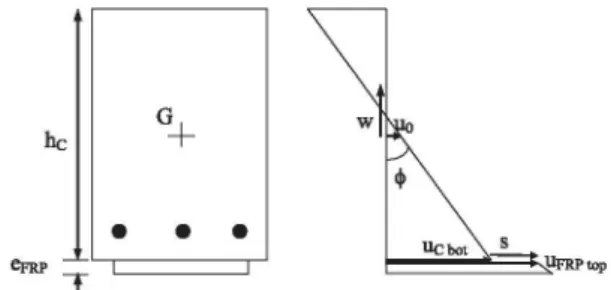
Firstly, the governing differential equations for the proposed problem are derived. On the basis of such equations the spectral method will be applied. Fig. 1 shows an FRP strengthened RC beam element. The subscripts C and FRP are used to denote quantities of the concrete beam and FRP strip, respectively; hc and hFRP are the

thicknesses of the concrete beam and FRP reinforcement, respectively.

For the derivation of the equations of motion, the following assumptions are made:

(a) No slip at the interfaces except at the RC beam-FRP plate interface in which an interface slip s is assumed as follows:

S — Ufgpfop — Ucfiot (1)

with uFRPtop and uc(,ot denoting the axial displacements at the

top of the FRP plate and at the bottom of the RC beam, respec-tively (Fig. 1).

(b) All layers take the same transverse displacement w(x, t)

w(x, z, t) = w(x, t) (2)

where z is the coordinate measured from the mid-plane. (c) The first-order shear deformation theory is adopted. Then, the

displacement field for axial and transverse motion is obtained by expanding the displacements in a Taylor series about the mid-plane displacements, u0(x, t) and w(x, t), as follows:

UC{X,Z, t) = tf0(X, t) - Z(j){X, t)

UFRP(X,Z, t) = tf0(X, t) - Z(j)(X, t) + S(X, t)

(3)

(4)

where uc and uFRP are respectively the axial displacements in the RC

beam and FRP plate. <p is the curvature-independent rotation of the beam cross-section about the y-axis. The coordinate z is measured from the mid-plane. These kinematic relationships are kept for the beam sections in which there is no FRP by removing the terms concerning the external reinforcement.

6FRP ^FRPtop

Using Eqs. (2)-(4), the linear strains for the different materials can be written as

(•xfRP = UQ>X — Zcj)x + Sx yxzfSP = W,x '

"fxzAD = SleAD

(5)

(6)

(7)

Here (•),* represents differentiation with respect to x and eAD

de-notes the thickness of the adhesive.

The linear constitutive model for the concrete beam and the FRP plate can be expressed as

<?x,c = Ec£x,c ^xz,c = Gcy^c

Txz,FRP = GfRPyxzFRP

(8)

(9) where the material constants, E and G, are referred to the concrete beam (C) or the external plate (FRP) depending on the material considered.

Calculation of bond shear stress between the FRP and concrete is very important in order to check the debonding failure mode. Its value along a certain length of beam can be expressed as a function of the axial force acting on the FRP plate. Based on the hypothesis on linear behavior of the adhesive interface, the following relation-ship can be assumed (Fig. 2)

t>a,AD — FpRptX — kfioS — GADy _xzfiD (10)

where FFRP is the axial force in the plate, kAD = GADleAD is the shear

stiffness of the adhesive and GAD is the elastic shear modulus of

the adhesive.

By using the previous relations, the strain energy for the strengthened sections is then obtained as

U = 2 (^(Tx,c£x,c + 'CXZicyxzCjbcdzdx

1 FRP

<?x,FRp£x,FRP + txzfRPyxzFRP ) bpRpdzdx

t>cz,ADyxz,AD ) bwdzdx (11)

where Z\ and z2 are the Z-coordinates of bottom and top surfaces

limiting each material, the variable b denotes the width of each material and L is the length of the strengthened beam.

From Eqs. (5)-(l 1), by application of Hamilton's principle the governing equations of the FRP flexural strengthened RC beam are obtained and can be written as

Su0:AnUo,xx + Bu<l>>xx-AFRpS,xx = 0 (12)

SW : A22W,xx + A22<t>,x = 0 (13)

&<t> : BnU0,xx ~ Dll4>,xx -A22W,x+A22(l> + BFRpStXX = 0 (14)

G sb

Ss : ApRpSxx - ApgpUo^xx + Bpgp(j>xx H = 0 ( 1 5 )

SAD

and associated force boundary equations can be expressed as

N = Anu0,x-Bucl>tx+ApRpStx (16)

Txz,ADbA

dx

FpRp+dFpRp

V =A22wx-A22<t>

M=-Buu0,x+DU(l - BpRpSy

N — ApRpSy + ApgpUox — Bp)

(17) (18) (19) JV, V, M and JV* are the stress resultants associated with the variables u0, w, 4> and s, respectively.

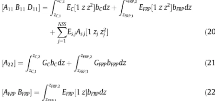
The stiffness coefficients, which are functions of the material properties and are integrated over the beam cross-section, can be expressed as

rzc,i [°ZFRP,2

[AnBnDn}= Ec[\zz2]bcdz+ EfRP[\ z z2]bFRpdz

NSS

^EsjAsjl^ZjZJ]

\A22] = Gcbcdz+ GpRpbpRpdz

[APRP BPRP] = / £pjy>[l z]bpRpdz •JZFRPJ

(20)

(21)

(22)

where the contribution of the internal reinforcement to the stiffness coefficients, /hi, Bn and Dn, has been included. NSS is the number of steel bars considered in the section, ESj and ASj are their elastic

moduli and section, respectively and Zj is the coordinate of each steel rebar.

2.2. Fourier expansion

We now perform a Fourier expansion of the field variables in the longitudinal direction

(tf0,w, <j>,s) = y^(u0,w, <j>,s)e ^\p-jkx ₍₂₃₎

where {0} = (u0, w, <j>, s) is an unknown constant vector and k is the wavenumber. This expansion, when inserted in problem (12)-(15), leads to a series of problems to solve in x for each Fourier mode k:

[W(k)]{u} = 0 (24)

The solution for this eigenvalue problem requires that the determinant of W must be zero which yields an 8th order charac-teristic equation for the wavenumber k whose solution gives the eight wavenumbers fe,.

The associated eigenvectors {0}, to each wavenumber fe, can be computed from Eq. (24) as:

{«},- =

/ u0\ /Rlt\ R2i

Rn

\sj{ \R4iJ

ai = {Ri}ai ( i = l , 2 , 3 , . . . , 8) (25)

where the eigenvector {0}, is normalized so that a component of the normalized vector {R,} becomes unity. The constants a, will be deter-mined to satisfy the associated boundary conditions. Once the eigen-solutions k( and {0}, are obtained to satisfy the eigenvalue problem in Eq. (24), the general solution to (12)-(15) can be written as:

{"(*)} = w(x) _4>{x)

v m I

= l{R,}{R2}---{Rs}]diag[e-^]

i=l,K,8

a2

w

= lW(x)]{A}

The eight unknown coefficients a, can be calculated as a function of the nodal spectral displacements, by evaluating Eq. (26) at the two nodes of the element, i.e., at x = 0 and x = I giving

{"1} {"2}

D(0)

D(L) W = |Ti]{A} (27)

where {i^} and {u2} are the nodal displacements of node 1 and node 2, respectively.

By eliminating the constant vector {A} from Eq. (26) by using Eq. (27), the general solutions can be rewritten in terms of the nodal degrees of freedom vector as

{u(x)} = [K][D(x)][7Y

-if ton

\{U2}J

<D

(28)

where [Nf is the matrix giving the shape functions for the displace-ment field.

By differentiating the spectral displacements with respect to x in Eq. (28) and using the force boundary Eqs. (16)-(19) to express the concentrated loads specified at two end-nodes of the element yields the spectral element matrix [/<]:

{/i}

{h}

F(0)

F(L) {A} = [T2]{A} = [T

2][T!]-{"l}\

{"2}

-*C)

(29)

3. Damage detection methodology

Structural damage identification is often formulated as an inverse problem. Given output responses (e.g. mode shapes or dis-placements) to specified input loads, changes in structural proper-ties (e.g. stiffness) from undamaged structural condition are inversely identified by minimizing an error or objective function. The objective function is generally defined in terms of the differ-ence between the response predicted by a computational model of the structure and the response measured from an experiment. When the response of the computational model matches that of the real structure, then predicted and actual properties of the tar-get structure would match each other as well. Therefore, suitable material parameters of the numerical model should be updated until that purpose is reached.

One of the keypoints to get the desired purpose is the suitable choice of the parameters involved in the objective function. Modal parameters obtained by dynamic testing have been widely used in structural damage identification since they are affected by the global characteristics of the structure. However, the interfacial debonding defect, which we want to detect, is purely local and modal characteristics are not very sensitive to local structural phe-nomena. Static measurements, such as strains and displacements, obtained by static truck load tests are more sensitive to the re-sponse in their vicinity and, therefore, they are better suited to determine local defects [24]. The use of static displacements is lim-ited by the accessibility of the structure and the number of loca-tions in which measurements would be needed. However, by means of a strain sensory system installed in the structure, a per-manent control can be carried out. Furthermore, technologies such as Bragg grating-based fiber optic sensors make this process easier. These kinds of sensors can provide a high sensitivity to debonding damage since they can be easily embedded at the FRP-concrete interface with a minimum of perturbation to the surrounding material. Compared to electric resistance strain gauge, the FBG sensor has the advantages of electromagnetic insensitivity, wave-length multiplexing, capability, miniature size, high sensitivity, good long-term stability and high reliability. The number of static measurements by static truck load tests is limited by the number of available sensors.

The sum of squared relative differences of static deformations at different locations of the structure might be employed to define the objective function:

E

j=i

ji.de) •

1,...,N£ (30)

in which the subscript j represents the jth measurement within the set of measurements carried out under a load case and : and

£expj are the computed and measured responses, respectively.

The updating parameters, de, defined for each element, e, are the uncertain physical properties of the NE elements of the numerical model, in our case, the reduction factors or damage indices affect-ing the RC-FRP interface stiffness. This damage index represents the relative variation of the adhesive element stiffness, (GAD)|J, compared to the initial value, (GAD)e:

4 = 1 iCAD)d

iGwf

The strain profile will change with the location of the trucks used in the controlled loading tests. Conceptually, different force transfer mechanisms may be activated according to the truck con-figuration. For this reason, to offer redundancy of experimental measurements and guarantee a reliable identification, different truck-load tests in various configurations should be executed. Then, different loading cases should be considered which means that different objective functions should be defined in the updating procedure, one for each loading case, such as follows:

* = E

in which the subscript i represents the set of measurements under load case i and the subscript j represents the jth measurement with-in the set.

In this way, the updating problem would be formulated in a multi-objective framework allowing capturing more information about the modeled problem as several sets of measurements are taken into consideration. All this will contribute to give a more reli-able solution to the problem [25,26]

An alternative way to Eq. (32) of evaluating the agreement be-tween experimental and numerical strains is by using the modal assurance criterion MAC [27]. Conventionally, the MAC criterion has been used to indicate the correlation between two sets of mode shapes in a normalized way. In our problem, for each load case i, the objective function will have the following expression: Fi = l-M4C({e„umii},{eew-})

{Emmy| {&exp,i j

\Enuny } |Emmy'} J 1 X&expjj X&expjj

(33)

This function, applied to each rth load case, has the advantage that each term is between 0 and 1. An index equal to zero means no correlation between the sets of experimental ({sexpj}) and numerical ({£num,i}) strains, while a value equal to one indicates a perfect correlation between the updated numerical model and the experimental results.

3.1. Damage detection without updated baseline model

make an accurate estimation of damage impossible. It is very likely that the inherent errors in the model will produce changes that are far greater than those produced by damage. Obviously, updating the baseline FE model of the undamaged structure using measured data would help to reduce model errors and improve estimation accuracy. However, the updating procedure is critical, since lots of measurements are needed for a large and complex structure in order to get a physically meaningful updated model. The difficulty increases, even for simple structures, when local parameters, such as strains, are used since a large number of measurements would be needed to get a good approximation. To overcome the problem of modeling errors, a method of structural damage identification is proposed here by adopting the same philosophy shown in [28]. In the proposed scheme, objective functions are formulated by using differences between measured strains of the damaged and undam-aged structure; the same approach is used for the numerical strains. All these methods are based on the fact that any error in the undamaged structure will also be present in the damaged structure and, therefore, will be removed. With this proposal, Eq. (33) would be formulated as follows

F,. = l-MAC(A{4m l.},A{4w.})

\M~4u

,,}

MM

,,}\

= 1" 7 f ^ 7 ^ 7 V (3 4)

(A{4m,i}TA{^umil.})(A{£^,.}TA{£^1.}) where

" l£n u m , i ) = l£num,i) — l£num,i) V-'-3)

A{4W'} = {4W'} " {4W'} (36)

and where subscripts 'num' and 'exp' refer to the numerical model with modeling errors and to the experimental results, respectively, and the superscripts 'd' and 'u' denote experimental and numerical values for the damaged and undamaged structure, respectively.

4. Multi-objective algorithm

The presence of multiple objectives requires finding the values of the damage parameter set {d} that simultaneously minimize the objectives. A multi-objective problem, in principle, produces a set of optimal solutions known as Pareto-optimal solutions instead of a single optimal solution. Each point in the Pareto optimal solu-tion set is optimal in the sense that improvement in one objective function leads to degradation in at least one of the remaining objective functions [29].

In the absence of any further information, one of these Pareto-optimal solutions cannot be said to be better than the others, which leads a user to find as many optimal solutions as possible. Solving multi-objective optimization problems is still a challenge. Evolutionary algorithms (EAs), such as genetic algorithms (GAs), are especially effective to solve multi-objective optimization prob-lems. A multi-objective GA simultaneously minimizes multiple objective functions, rather than using arbitrary weighting factors to combine them to a single-objective function. A considerable amount of research has been done with success in this area due to the difficulty of conventional optimization techniques being ex-tended to multi-objective optimization problems. Because of this, several multiobjective EAs have been proposed in recent years [30-32]. However, evolutionary techniques require a relatively long time to obtain a Pareto front of high quality.

Recently, approaches based on particle swarm optimization (PSO) have received a great deal of attention in engineering prob-lems. This method, originally proposed in [33] for optimization, is a stochastic optimization technique which is inspired by the

behavior of bird flock, and is considered as an evolutionary algo-rithm by its authors [34]. Although PSO is relatively new, the rela-tive simplicity, the fast convergence, the few parameters to be adjusted and the population-based feature [35] have made it a high competitor in solving the multi-objective problems when com-pared to other methods.

In the same way as traditional evolutionary algorithms, PSO is initialized with a swarm of random particles and then, using an iterative procedure the optimum is searched for. For every updat-ing cycle, each particle is updated such that it tries to emulate the global best particle, known as gbest, found so far in the swarm of particles, and the best solution, known as pbest, found so far by particle n, i.e., the number of pbest particles agrees with the num-ber of particles in the swarm. To perform this, self-updating, equa-tions are used as follows:

v„=w-v„+c-l-r1- (pbestn - x„) + c2-r2- (gbest - x„) (37)

x„ = x„ + v„ (38) where v„ is the particle velocity, xn is the current position of particle

n, w is an inertia coefficient balancing global and local search, rx and r2 are random numbers in [1 ] and Oi and c2 are the learning factors

which control the influence of pbestn and gbest on the search

pro-cess. Usually, values equal to 2 are suggested for cx and c2 for the

sake of convergence [36]. Additionally, the velocity is limited to a maximum value with the purpose of controlling the global explora-tion ability of particle swarm avoiding it moving towards infinity. Eqs. (37) and (38) represent the original PSO algorithm although some variations have been proposed [37]. Since an individual ob-tains useful information only from the local and global optimal indi-viduals, it converges to the best solution quickly. PSO has become very popular because of its simplicity and convergence speed.

The inertia weight w is an important factor for the PSO's conver-gence. It controls the impact of the previous history of velocities on the current velocity. A large inertia weight factor facilitates global exploration while a small weight factor facilitates local explora-tion. Therefore, it is advisable to choose a large weight factor for initial iterations and gradually reduce the weight factor in succes-sive iterations. This can be done by using

where wmax is the initial weight, wmin is the final weight, itermax is

the maximum iteration number, and iter is the current iteration number.

However, although not so extended like GAs in solving multi-objective problems, its high convergence speed and feasibility of implementation make PSO an ideal candidate to implement a structural health monitoring technique in real time in a multi-objective context.

4.1. Multiobjective particle wwarm optimization (MOPSO)

The PSO proposed here for multi-objective optimization should aim to preserve population diversity for finding the optimal Pareto front and to include the feature of local fine-tuning for good popu-lation distribution by filling any gaps or discontinuities along the Pareto front. Furthermore, the selection process of the best parti-cles with the purpose of extending the existing particle updating strategy in PSO to account for the requirements in multi-objective optimization should be solved too.

Due to the similarity of particle swarm and other evolutionary computation methods, such as genetic algorithms, some multiob-jective handling techniques can be adopted to the modified PSO.

In this section, the features of the proposed multiobjective particle swarm optimization algorithm will be described, and details of its implementation will be presented.

4.1.1. External repository

Following the same guidelines as in SPGA [40], in the proposal, elitism is implemented in the form of a fixed-size archive or repos-itory to prevent the loss of good particles due to the stochastic nat-ure of the optimization process. The archive is updated at each cycle, e.g., if the candidate solution is not dominated by any mem-bers in the archive, it will be added to the archive. Likewise, any ar-chive members dominated by this solution will be removed from the archive.

Furthermore, in order to maintain a set of uniformly distributed non-dominated particles in the archive, the average linkage meth-od [41 ] has been chosen. The basic idea of this methmeth-od is the divi-sion of the non-dominated particles into groups of relatively homogeneous elements according to their distance. The distance d between two groups, gx and g2, is given as the average distance

between pairs of individuals across the two groups.

d

=]s^\ E IK-MI (

°)

1511 1521 ii e g ] ]i2 e2,

where the metric • reflects the distance between two individuals ii and i2.

Then, following an iterative process, the two groups or clusters with minimal average distance are amalgamated into a larger group until the number of clusters is equal to the maximum permitted capacity of the repository. Finally, the reduced non-dominated set is computed by selecting a representative individual per cluster, usually the centroid. With this approach a uniform distribution of the grid defined by the non-dominated solutions can be reached.

4.1.2. Selection ofpbest and gbest

In MOPSO, gbest and pbest play an important role in guiding the entire swarm towards the global Pareto front. Contrary to single objective optimization, the gbest and pbest for multiobjective opti-mization exist in the form of a set of non-dominated solutions. The selection of pbest follows the same rule as in traditional PSO but applying the Pareto dominance concept.

In MOPSO there is no such thing as the best position vector such as in standard PSO. There are several equally good non-dominated solutions stored in the external repository. The selection of an appropriate gbest is critical for the search of a diverse and uni-formly distributed solution set. In order to promote diversity and to encourage exploration of the least populated region in the search space, the choice of gbest is performed by the roulette wheel selection scheme based on fitness assignment. For its application, all the particles of the external repository are assigned weights based on their fitness values; then the choice is performed using roulette wheel selection. The fitness assignment mechanism for the external population proposed by Zitzler and Thiele [40] has been used in the proposed algorithm. According to this mechanism

each individual m in the external repository is assigned a strength si proportional to the number of swarm members which are dom-inated by it, i.e.

where nm is the number of swarm members which are dominated

by individual m and JV is the size of the swarm. The fitness value of the individual m is the inverse of its strength. Therefore, non-dominated individuals with a high strength value and, therefore, lo-cated in regions more densely populated are penalized and have a lower probability of being selected.

5. Numerical study

For the purpose of evaluating the methodology presented, both numerical and experimental studies were carried out. For the ini-tial study, the damage identification procedure was checked by assuming different simulated damage scenarios.

In the numerical study, a very detailed continuum-based 2D fi-nite element (FE) model has been used to generate the pseudo-experimental strains. This model would not be suitable for the damage detection algorithm due to its high computational cost. In the FE model, plane stress elements were used for the concrete, adhesive and FRP, while the internal steel reinforcement was mod-eled using truss elements. Loss of shear transfer in the debonded zones was simulated by reducing the mechanical properties of the adhesive, i.e. the shear modulus for the adhesive was reduced to a very small value. The geometric dimensions and the reinforce-ment layout in the sections are illustrated in Fig. 3 and the material properties used in the model were assigned as follows: (a) for concrete and steel reinforcement, the elastic moduli were taken to be 25,000 MPa and 210,000 MPa, respectively, and Poisson coefficient for concrete is 0.2; (b) for FRP external reinforcement, the elastic modulus and Poisson coefficient were taken to be

E= 165000 MPa and o = 0.35, respectively, and the thickness is

0.0012 m. For the analysis, the elastic modulus in the direction perpendicular to the fibers is assumed to be one-tenth of that in the direction of the fibers. This assumption is generalized for all calculations, since no data were available for the transverse elastic modulus; (c) for adhesive, the shear modulus was assumed to be G = 4300 MPa and the thickness eAD = 0.0018 m.

Yet, in order to keep a suitable level of refinement of the FE model with a reasonable computational effort, the mesh is limited to four elements through the thickness of the adhesive layer and two elements through the thickness of the FRP layer reaching a to-tal number of 81874 nodes and 78760 finite elements. Since only strains under service loads were used in the damage identification procedure, a linear elastic analysis was performed.

0.275 m 0.265 ml

•* »• * w

V !! I

0.20 m

3 cm

0.74 m

6 cm

1.3 m 1.88i

0.045 1 % 0.008 m ^

^(j) 0.01 nr-Q, 0.15 m

0.15 1

Fig. 3. Geometry and loading schemes for the numerical study.

Load at the midspan

Position along the FRP strip

Fig. 4a. FRP strain distribution under a concentrated load applied at the midspan.

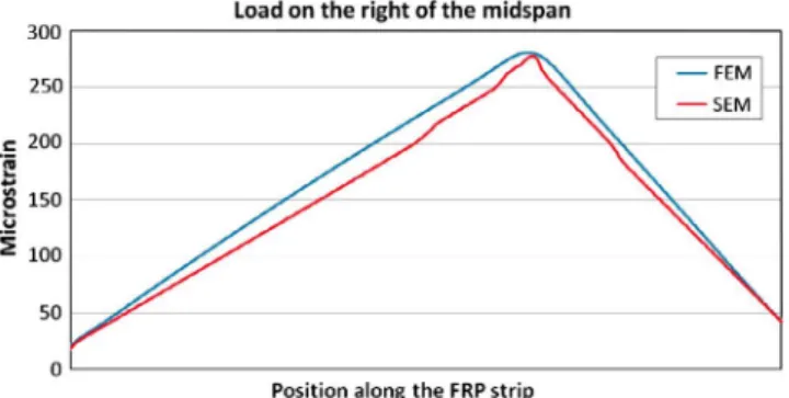
Load on the right of the midspan c 200

S 150

Position along the FRP strip

Fig. 4b. FRP strain distribution under a concentrated load applied on the right at

the midspan.

300 250

Load on the left of the midspan

S 150

Position along the FRP strip

Fig. 4c. FRP strain distribution under a concentrated load applied on the left at the

midspan.

However, in spite of this, the non-baseline model was updated from the FE 'pseudo-experimental' results of the control beam, which means that modeling errors are present in the numerical model used for the damage identification. Taking as basis the FRP strains, the average level of modeling errors in the baseline spectral

model in comparison to the FE model for the control beam is de-fined as

Error: = ||{£f£,i}-{£5£,i}||

IKWII2

in which {EFE,,-} and {ESEJ} are the finite element and spectral strain vectors, respectively, for the ith load case.

From Eq. (42), the relative errors for the three loading cases, midspan, left and right, are 1.55%, 1.87% and 2.63%, respectively, and, therefore, those errors are assumed in the damage identifica-tion procedure.

Once numerical and pseudo-experimental results were gener-ated for the control beam, three new sets, one for each load loca-tion, of pseudo-experimental strains at the FRP strip were generated with the FE model as previously but assuming that interfacial damage is present. Specifically, two damage scenarios (different locations and degrees of damage) were considered. A sin-gle damage scenario due to a debonded area at the FRP-concrete interface of length equal to 3 cm and a multiple damage scenario due to two simultaneous damages of length equal to 3 cm and 6 cm, respectively. The location of these two damage areas is shown in Fig. 5. A three-objective optimization problem has been carried out as shown in previous sections to identify the debonded areas in the two damage scenarios. For this, the three objective functions, corresponding to each one of the loading cases, were for-mulated according to Eqs. (34)-(36), i.e. without considering an updated baseline spectral model. The spectral element meshes for both damage scenarios are shown in Fig. 6. Each node would correspond to a sensor in which the strain is measured. The meshes have been defined to be more refined in the proximity of the inter-facial failure region and to be coincident with the points of appli-cation of the loads. Furthermore, an element has also been

3 cm

0.74 m

T

-2 m

(a) Single damage scenario

3 cm

0.74 m

r

6 cm

1.3 m

1.88 m 2 m

(b) Multiple damage scenario

chosen coincident with the debonding area. The multi-objective problem was solved by using the PSO algorithm developed in Sec-tion 4.1. Selected parameters for the applicaSec-tion of the PSO algo-rithm are the following: Cognitive parameter cx = 2, social

parameter c2 = 2, initial inertia weight wmax = 0.95, final inertia

weight wend = 0.4, maximum velocity ^m a x=100. Twenty simula-tion runs were performed for each case in order to study the statis-tical performance and a random initial population of 50 individuals was created for each of the 40 runs. Furthermore, a size of 50 was adopted for the external repository. Each design variable or dam-age variable, d, € [0,1] for each ith element was coded into a 3-bit binary number, obtaining a resolution of 0.125, which is accept-able for a suitaccept-able estimation of damage.

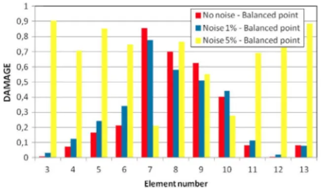
Figs. 7 and 8 show the damage distribution at the concrete-FRP interface for the two damage scenarios. In both cases, damage is assumed to happen at the intermediate regions of the concrete-FRP interface, not at the vicinity of the concrete-FRP ends. This means that the damage variable will be only calculated for elements 3-13 and 3-16 for the single and multiple damage scenarios, respec-tively, according to Fig. 6. Multi-objective evolutionary algorithms can be classified as a posteriori. When the Pareto optimal solutions to the multi-objective problem are known, the user has to choose one of the solutions according to the importance rating of the sev-eral objectives. This rating is based on higher level information that has not been built into the model that is to be optimized. In our problem the objectives are in the range [1] and we assume that the ranges of values covered by the Pareto front in each objective are equally important. Furthermore, the three objective functions have been defined in a similar way dependent on strains for three

I No noise - Balanced point I Noise 1% - Balanced point Noise 5% - Balanced point

7 8 9 Element number

Fig. 7a. Damage distribution for the single damage scenario when the balanced point is chosen.

load cases. According to this, two alternatives have been evaluated to choose the Pareto point. The first, denoted here as "balanced point" (Figs. 7a and 8a), consists in choosing as single solution the Pareto point for which the values of all objective functions are closer: min(|Fi • I f 2 • | F3- F l | (43)

With this approach, all the objective functions are valued equally. In the second alternative, denoted here as "closest point" (Figs. 7b and 8b), from the set of Pareto optimum solutions ob-tained, the chosen one is that minimizing the following expression

n+n+n

i.e., the chosen Pareto point is the closest to the origin.

Damaged element

!©* @ © '®(M)<Z)<*)®V®' 6 '®'$W&

\

Damaged element Damaged element

Fig. 6. Spectral element meshes.

Fig. 7b. Damage distribution for the single damage scenario when the closest point

is chosen.

-Mi-• No noise - Balanced point • Noise 1% - Balanced point

Noise 5% - Balanced point

• 1 .

l l

_

1

I

3 4 5 6 7 8 9 10 11 12 13

Element number

Fig. 8a. Damage distribution for the multiple damage scenario when the balanced

point is chosen.

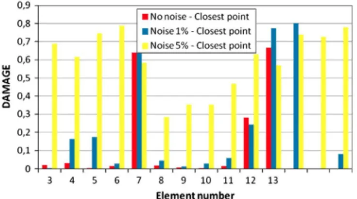
7-J-k-• No noise - Closest point • Noise 1% - Closest point Noise5% - Closest point

L

--*

1

—

1

3 4 5 6 7 8 9 10 11 12 13 Element number

Fig. 8b. Damage distribution for the multiple damage scenario when the closest

point is chosen.

Figs. 7 and 8 illustrate that the debonded zones, element 8 at the single damage scenario and elements 8 and 14 at the multiple damage scenario, are easily identified when noise is not present. Furthermore, in the multiple scenario, the detected severity is higher in the wider damaged area. No significant difference is ob-served between choosing to represent the balanced point or the closest point. Therefore, with only a limited number of available strain readings the damage detection was performed in a simple and fast way compared to the large number of elements involved in a finite element analysis, unacceptable from a practical point of view. Of course, the reliability of the method would improve in field monitoring by using more measurement points.

In a further study, for each damage scenario, the "measured" FRP strain responses of the strengthened beam before and after damage were generated with 1% and 5% of noise. For the two dam-age scenarios, damdam-age estimation was performed again through a spectral model updating procedure using a three-objective formu-lation with the same proposed objective functions in Eqs. (34)-(36) for purposes of comparison. This formulation also includes model-ing errors in the baseline model and the same parameters for MOPSO as in the unnoisy case were adopted. Figs. 7 and 8 show the results for the two damage scenarios and for both noise cases, 1% and 5%. Predictions with 1% noise are good and do not differ from the unnoisy case. However, when an artificial noise of 5% is introduced a sparseness in the damage distribution is obtained for all the elements, the identification of the damaged areas being impossible. This is due to the fact that the change introduced by the level of noise is higher than the real strain difference between the undamaged and damaged cases and, therefore, the real damage detection turns out to be difficult in that case. The change introduced in the strain distribution along the FRP length by minor debondings is small and, therefore, a perturbation such as that due to a significant noise might affect the predictions. However, the noise involved in strain measurements is small and, furthermore, the noise can be decreased by repeating the measurements a num-ber of times.

In the previous studies the spectral element meshes were adapted to the debonded zones in such a way that the level of refinement was higher in the areas closest to the damaged inter-faces and, furthermore, one element was always chosen coincident with the damaged area. However, damages are not likely to be exactly the same size as elements in the numerical model; there-fore, the effect of mismatched element size should be investigated for practical application. In order to investigate this effect, taking as a base the same single damage scenario from Fig. 6a, a more real-istic case was carried out in the sense that all the elements were considered to be almost of the same length equal to 10 cm and not necessarily exactly coincident with the damaged areas (Fig. 9). The uniform element length is only slightly modified at the vicinity of the loading points to locate nodes coincident with these points. From an experimental point of view this would be the equivalent of installing a single cable on an FRP laminate with multiple FBG sensors equally spaced along its length to monitor the health of an FRP strengthened beam without previous knowl-edge of the areas in which debonding might originate. Each strain sensing point is coincident with a node of the spectral mesh (Fig. 9). As in the previous studies, in the numerical procedure it is assumed that damage might only happen at the intermediate re-gions of the concrete-FRP interface, not at the vicinity of the FRP ends. This means that only elements 3-12 in Fig. 9 were assumed to be potentially damaged. The damaged area extends over a par-tial length into the fifth element. Fig. 10 shows the damage predic-tions for the single damage case, unnoisy and with 1% and 5% noise, respectively. Only the balanced Pareto point is represented for sim-plicity although the conclusions would be very similar in the case of choosing the closest Pareto point. The same conclusions as in the previous cases might be extracted. Damage is perfectly identified when the level of noise is low but false warnings appear when noise increases.

6. Experimental damage identification

0.275 m 0.265 m

h

4

10.06 0.44 0.125 0.1 0 075 0,1 0.1 0.1 0.1 0.065 0.0.15 0,1 0 54 0.06i

r

® ® ® 0 ® (!) (!) ® © © @@ © @l

\

Damaged element

Fig. 9. Quasi-uniform spectral element mesh for the single damage case.

1

0,9

0,8

0,7

3°<

1 0 , 5

Q 0,4 0 , 3 - I

:

;lhl=

I No noise - Balanced point I Noise 1 % - Balanced point

Noise5%- Balanced point

U

3 4 5 6 7 8 9 10 11 12

Element number

Fig. 10. Damage distribution for the single damage scenario when a quasi-uniform

mesh is used.

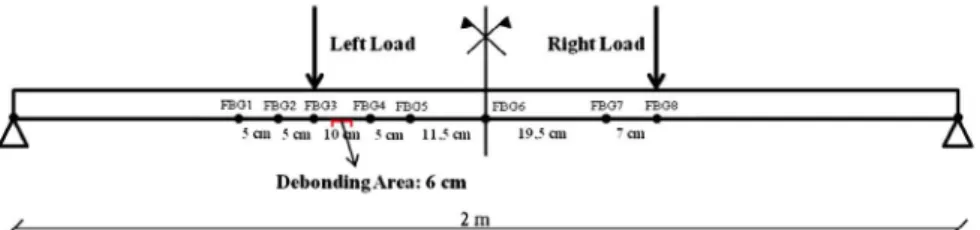
under service loads has been used. Specifically, two specimens were tested, a control specimen without debonding and a speci-men in which a debonding of length 6 cm was induced at the loca-tion shown in Fig. 11.

To determine the strain profile at the FRP laminate a network of FBG sensors was distributed along its length, such as shown in Fig. 11. As observed, more sensors were placed in the proximity of the debonding zone.

Two loading configurations were used consisting of a concen-trated single load placed at two different locations at a distance of 26.5 cm on the right and on the left, respectively, from the mid-span section. The load was applied alternatively at these two loca-tions under three controlled load levels. During the first two levels, 8 kN and 14 kN were applied and then the beams were loaded to failure. During each stage of testing, the FBG strains, the applied load and midspan deflection were recorded continuously to be used in the proposed damage identification technique.

Practically, the concrete remained uncracked under 5 kN and because of this strain profiles corresponding to lower load levels were used to check the proposed technique since the focus of this research was damage detection under service conditions.

To apply the proposed damage detection strategy, a very simple spectral numerical model was implemented originally for the con-trol beam. This model consists of 11 elements as shown in Fig. 12; as usual, nodes were chosen to be coincident with the sensor loca-tions and loading points. Numerical linear elastic analysis was as-sumed to be suitable for our purposes.

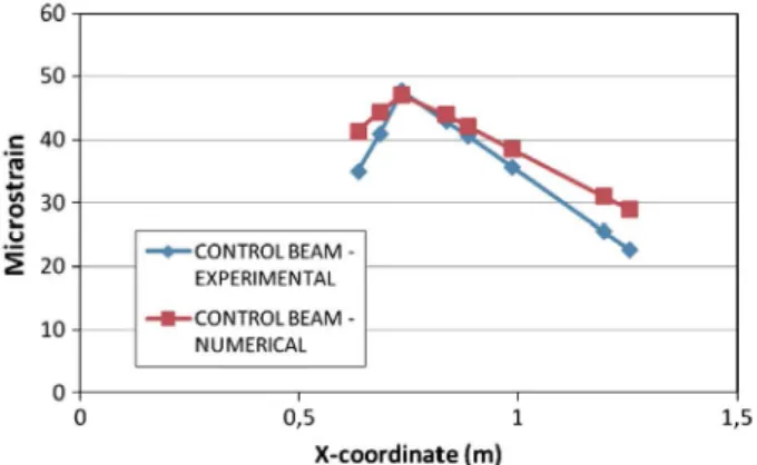
Figs. 13a and 13b show the comparison of the experimental and numerical FRP strain profiles obtained for the control beam for both load locations when the load reached a value of 4 kN. Only the values corresponding to the location of the sensors are shown since they are the only values experimentally obtained. As in the previous section, although some differences can be observed be-tween the numerical and experimental strain profiles, a non-base-line numerical model was updated from the experimental results of the control beam and, therefore, some modeling errors are pres-ent in the numerical model used for the damage idpres-entification. The same model of Fig. 12 is used for the debonded beam but including a damage variable to be determined in those elements included be-tween nodes coincident with FBG sensors (elements 3-9 according to Fig. 12). Real damage should be detected at element 5 according to the numbering in Fig. 12.

A two-objective optimization problem, defining one objective function for each load location (left and right), has been solved to identify the debonded area in the experimental damage scenario. The multi-objective problem was solved by using the PSO algo-rithm developed in Section 4.1 with the same parameters used in the numerical examples. The damage indices for each element computed with the multi-objective algorithm are shown in Fig. 14. The damage index values plotted in the figure were calcu-lated from the mean values of the "closest points" of the 40 runs. Apparently from the figure, the damaged area is identified since

1

1

k

i

5 an 10 en 5 an 11.5 an

Debonding Area: 6 cm

/- 2m -/

0.265 m 0.265 m

f

I 0 06

LHMH

= 0 115 0 195 0.07

I ® — © W < S ) W (?) ' V ®"

\

Damaged element

Fig. 12. Spectral element mesh for the experimental beams.

60

50

40

30

20

10

—•— CONTROL BEAM -EXPERIMENTAL

- • - CONTROL BEAM -NUMERICAL

>

^

j^y

^r

tT

1 1

0,5 1

X-coordinate (m)

1,5

Fig. 13a. FRP strain distribution under a concentrated load applied on the right of

the midspan. Experimental control beam.

60 50 c 40

2 S 30 u

I 20

10

0

-CONTROLBEAM-EXPERIMENTAL -CONTROL

BEAM-NUMERICAL

^

0,5 1 X-coordinate (m)

1,5

Fig. 13b. FRP strain distribution under a concentrated load applied on the left of the

midspan. Experimental control beam.

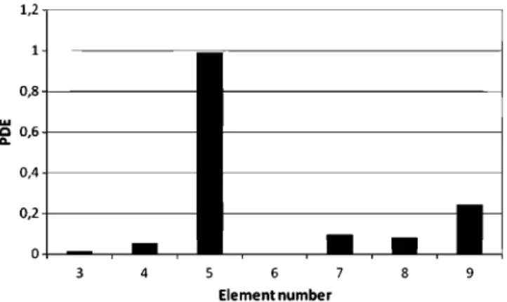
the peak values appear close to the debonded zone (element 5). However, damage values higher than zero appear at the other ele-ments too. Furthermore, these indices might vary from one run to another considering all the numerical and experimental uncertain-ties of the method. Taking these values to be the limiting values above which damage is inferred might lead to erroneous conclu-sions. To avoid this, after estimating the damage distribution of the debonded beam, a probability of damage existence (PDE) was derived from the statistical distributions of the damage indices or element stiffness parameters of intact and damaged beams

5 6 7

Element number

Fig. 14. Computed damage distribution for the experimental beam.

[42,43]. The basic idea of this approach is to compute the probabil-ity of a damage index at a confidence level. PDE takes values be-tween 0 and 1 in such a way that values close to 1 indicate that the element is most likely to be damaged while if the PDE is close to 0, the damage of the element is very unlikely. With this ap-proach, the probability of detecting damage in an undamaged member and the probability of not detecting damage in a damaged member should be both tolerably small.

The statistical distribution (mean and standard deviation) for the damaged beam was obtained when the damage identification procedure was applied. To obtain a statistical distribution of the element stiffness parameters of the undamaged control beam, an additional noise of 2.5% was included in the measured experimen-tal strains of the control beam and the proposed multi-objective algorithm was applied defining the objective functions from Sec-tion 3.1 in the following way: Undamaged experimental strains in Eq. (36) are taken from the experimental measurements on the control beam while damaged experimental strains are obtained from the previous ones by including an additional noise of 2.5%. In Eq. (35), undamaged numerical strains are obtained from the intact numerical spectral model while damaged numerical strains should be updated during the optimization procedure to obtain a stiffness parameter statistical distribution of the undamaged structure (control beam) for a level of uncertainty of 2.5%. This value was chosen considering that the maximum relative error calculated from Figs. 13a and 13b according to Eq. (42) is slightly higher than 2.5%.

1.2

1-

0,8-u j

Q

0,6-Q.

0,4-

0,2-

0--3 4 5 6 7 8 9 Element number

Fig. 15. Probability of damage existence for the experimental beam.

shown in Fig. 15, the probabilities of damaged elements (element 5) are very high while those undamaged elements have a probabil-ity far less than 1. Thus the proposed method can identify most likely damaged elements.

7. Conclusions

An automated methodology, which can operate in an unsuper-vised mode, has been proposed to identify minor damage in FRP flexural strengthening RC beams due to interfacial debonding at intermediate sections. The application of a proposal like this turns out to be essential to prevent sudden and brittle FRP bond failure modes originated from intermediate sections at FRP strengthened structures and, therefore, is consistent with the strong existing de-mand on developing high performance structures, able to monitor the mechanical properties during service condition. Some of the strong points of the proposed method might be summarized as follows.

The success of these kinds of damage identification methodolo-gies depends strongly on the use of a suitable simplified model of the structure to be evaluated. For this reason, a one-dimensional simplified spectral model has been implemented to simulate the behavior of RC beams strengthened with FRP. Starting from this model, the detection procedure has been formulated to be depen-dent on FRP strain distribution since damage to be detected is a local phenomenon and modal parameters are not suitable for this purpose. The use of experimental strains instead of modal variables decreases the level of uncertainty of the procedure. The method has been developed in a multi-objective framework and without the need to know an updated baseline model. This last aspect can be advantageous in cases and situations in which the formula-tion of a suitable updated physically meaningful model can be very difficult. Furthermore, the formulation of the model updating prob-lem based on several objective functions allows working with strain responses under various configurations provided by moving loads, which can activate different force transfer mechanisms and offer redundancy of experimental measurements, contributing in this way to increase the reliability of the procedure.

A modified version of the standard PSO algorithm has been proposed with the purpose of improving its performance when applied to a multi-objective framework. With properties such as fast convergence, storage and continuous modifications of poten-tial solutions in an external repository, this new version can evolve as an alternative and preferable tool for structural damage identi-fication in multi-objective problems over other algorithms such as evolutionary algorithms. Its high convergence speed and feasibility of implementation make it an ideal candidate to implement a structural health monitoring technique in real time.

Considering the local nature of the studied damage, damage predictions with the proposed methodology were successful in cases in which experimental uncertainty due to noise is lower than the changes at the FRP strain distribution introduced by local dam-age even for non-updated numerical models. Because of this, it ap-pears to be very promising as a non-destructive evaluation technique when combined with FBG sensors which are able to measure strain locally with high resolution and accuracy.

Acknowledgements