A comparative analysis of fault detection schemes for stochastic continuous-time dynamical systems

in Science and Engineering, CMMSE 2008 13-17 June 2008.

A comparative analysis of fault detection schemes for

stochastic continuous-time dynamical systems

P e d r o J. Zufiria1

1 Departmento de Matemdtica Aplicada a las Tecnologias de la Information, ETSI

Telecomunicacion, Universidad Politecnica de Madrid

emails: [email protected]

Abstract

This paper addresses a comparative analysis of the existing schemes for fault detection in continuous-time stochastic dynamical systems. Such schemes prove to be efficient when dealing with specific types of fault functions; on the other hand, they show very different performance sensitivity when dealing with new fault profiles and system noise. The study suggests the use of a combined scheme, supervised by a high level decision rule set.

Key words: fault diagnosis, continuous-time stochastic dynamics, moving angle, mean estimator

1 Introduction

Fault detection schemes have deserved much attention in the last two decades [2, 7, 8, 11]. Among them, some model-based schemes make use of explicit analytical models for redundancy checking in two directions. On one hand, stochastic discrete-time models combine statistical schemes with geometrical tools in the design and characterization of detection algorithms for linear systems [2, 7, 8]. On the other hand, deterministic continuous-time models have shown to be suitable for nonlinear system modelling [1, 5, 6, 12, 14].

Continuous-time stochastic models in system fault diagnosis have recently been em-ployed for considering system and sensor noises and disturbances, in order to construct new detection and isolation algorithms [3, 4, 9, 10].

In this work a comparative analysis of these existing schemes for fault detection in continuous-time stochastic dynamical systems is presented.

2 Systems formulations and parity checking

The existing schemes for the fault detection problem in nonlinear time-variant dynam-ical systems, consider different forms of the following model:

x(t) = f(x(t)Mt),6o,t)+v(t) + B(t-T0)<i>(t),

x(0) = x0

(1)

where x(t) G W1 is the system state, u(t) G Em is the control input, and the Gaussian

white noise random vector 77 : E+ —> En represents external disturbances and modelling

errors.

The function / e C1^71 x Rf f lx E+,Mn), which represents the dynamics of the

nominal model is assumed to have general form in [3, 4]. On the other hand, [9] only considers scalar systems, whereas [10] allows it only to have the form

0 1 0 0 /(x,u,0o,£) = Enx(t) + eng(x,U,$Q,t), En =

0 0 0 " 0 1 0 _

5 en —

" 0 ' 0

0

. l \

being g(x)ui9o)t) a scalar function.

Concerning the types of faults gathered by the model, in [3, 4] any additive faults are considered due to some fault stochastic process <\> : M+ —• Rn which represents the

changes in the system dynamics. B(t ~TQ) is a diagonal matrix representing the time profile of the fault (see [4] for details).

Alternatively, in [9, 10] the failure function is only allowed to be scalar so that

B(t - TQ)(jy{t) = ens(t - T0)^(x, w, $ue0i t)

so that ip(x, it, 91, <9o, t) is a scalar fault function. In this context, parametric faults (due to a change in the parameter vector from #o to 0\ at the unknown instant To) are only addressed. Such changes are modelled in additive form with B(t — To)<£(£) = s(t - To), step function, and

4>(t) = #a;(i),u(t),0i,0o,<) = f{x(t)Mt)^ut) - f{x(t),u{t),6Q,t).

2.1 Parity checking residual

(2)

All approaches assume state availability, so that parity-checking is carried out via the Luenberger observer type structure ([3, 10, 13]):

x(t) = -A(x(t) - x(t)) + /(x(t),u(t),t), x{0) = zo, (3)

where x(t) € Mn is the state estimation and the matrix A = diag(Ai,... , An), with

Xt > 0, i = 1,... ,n.

Due to state availability, function /(x(-), •, •) is used instead of /(£(•),-,-) as it would correspond to a proper Luenberger observer.

Subtracting observer (3) from system (1), and since the MS derivative is a linear operator, we can obtain the differential equations system which explains the evolution of the residual, e(t) = x(t) - x(t):

e(t) = -Ae(t) + V(t) + B(t - r0)<fti), 6(0) = 0. (4)

The solution of such differential equations system (4) is

e(t) = / e-A*£-r>77(T) dr+ l e ^ ^ B ^ - T0)4>(r) dr,

Jo Jo

and the analysis of e(t) under different hypotheses forms the basis of the detection schemes.

3 Scheme p r o p o s e d in [3]

The FD scheme proposed in [3] is oriented to detect changes in the residual mean. The following hypotheses test is proposed:

Ho : E[e(t)] = feA^-^E[r)(r)}dr (5)

Jo

H

: E[e(t)]* f e^^E^dr.

In order to apply such test, a mean estimator, fj,(t) : R+ —• En must be chosen

first, and the following continuous time estimators of the mean are proposed in [3]:

• fia(t) =e(t).

• ^b{t) = \!le{r)dr, t > 0.

• McW = T//_Te(T)d r> t>T

-• / i d W = / o ^ * -T^ ( r ) d T , p<0.

Here we will not consider /Xd(i), since it is a biased estimator.

Once their probability distribution is determined, the acceptance region of the test, £(£), is derived defining a ball B(t), centered in the mean of the estimator under the hypothesis of no fault E[n(t)/Ho] and fulfilling

P(ti(t) e B(t)/H0) = 1 - 7 ,

where 7 is a small value previously chosen that constitutes the test size, and it is consequently the false alarm rate at each instant t.

As a consequence, the following test decision is derived: If fx{t) £ B(t) then it is

likely a FAULT has occurred in the plant.

Finally, the instant of time when the fault is detected is defined as the random variable

Ti = M{t>T0/»(t)$B(t)}. (6)

A complete analysis of the detectability properties of the scheme is also provided in [3]. Some of the claimed properties will be analyzed here from a comparative point of view.

4 Scheme proposed in [10]

The scheme proposed in [9, 10] is aimed to detect small changes in the system param-eters. For doing so, it employs the so called moving angle between the residual process and a reference signal, based on the moving inner product between two scalar processes

a(t) and /3(i), which is defined as

< ^ > T ( « ) 4

f E[a(r)0(r)] dr.

Considering small variations on 0, the fault process </>(t) is linearly approximated

0Or(i),u(t),0i,0o,t) « K-<p(x{t)M*)>0o,t)

so that if the direction of the parameter change 0\ - OQ is known, the profile can be determined, except for a proportionality constant.

Considering state space availability, ip(t) is computed and

<PLp(t)= / ' e -A< * -TV ( r ) dr.

Jo '0

serves as a reference signal to compute the cosine

<e><PLP>r(t) K cos(e, <pLP)T{t) =

H I r M • W^Lphit)

V + IIVLPII^)

which can be large enough provided the system noise variance is small.

In [10], an estimator is proposed for this cosine-based scheme and its mean and variance are computed in order to define the corresponding regions of the test for both detection and isolation of faults.

5 Comparative simulations

5.1 S y s t e m definition

In this section we comparatively illustrate the application of the detection approaches to a bidimensional system, the so called van der Pol oscillator system. Let us consider the system

xi(t) = x2(t)+r)i(t)+0{t-To)<l>i{t) M

x2(t) = 2^{l-lix\{t))x2{t)-uj2xl(t)^m{t) + (3{t'TQ)^{t),

with initial condition x(0) = (1,0)'. It describes the dynamics of the van der Pol oscillator, taking into account external disturbances via the vector random process

r)(t) = (Vi{t))V2(t))'- Such processes are assumed to be mutually independent, and

dis-tributed as white Gaussian noise (WGN), with zero mean and autocorrelation function

where a^ = tf2 = 0-1.

We take to = 1, ( — 1, and \i — 1, so that the trajectories of the system in normal operation tend to a limit cycle (corresponding to the periodic solution of the deterministic van der Pol oscillator).

Both additive faults and parameter changes in a;,£ and \i will considered. First, we are going to define the setting of the employed detection schemes.

5.2 Detection schemes tuning parameters

We will consider that both schemes can measure the system state space variables, although Scheme 1 will only employ the second component X2(t) as seen below. The parity-checker is selected with Ai = A2 = —5 and initial condition x(0) = (1,0)',

5.2.1 Detection Scheme 1

Concerning the detection scheme proposed in [3], we will apply the mean estimators

1 [l 1 /"*

Mi CO = £2CO, M2(0 = 7 / e2{r)dr, fi3(t) = - / e2{r)dr,

t Jo 1 Jt-T

(8)

with T = 10 for the third estimator.

The selected test sizes have been 71 = 72 = 0.001 (this value is only critical for

Hi (t) as commented later) providing the tests acceptance regions

- 3 . 2 9 ^ ^ / ^ ( 0 , 3 . 2 9 y / V ar t H / H o( t ) i = 1,2.

When any of the mean estimators crosses the frontier of its corresponding accep-tance region an alarm is shot, indicating that it is likely a fault has occurred in the system.

5.2.2 Detection Scheme 2

Concerning the detection scheme proposed in [10] > we have considered the moving angles (with window size T = 10) corresponding to the three parameters with parameter values

K^ — K^^K^ — 0.2, and 71 = 72 = 0.05. One has to say that this parameter tuning

has been critical to avoid false alarms whereas keeping sensitivity to the faults.

Again, when any of the angle estimators crosses the frontier of its corresponding acceptance region an alarm is shot, indicating that it is likely a fault has occurred in the system.

5.3 Additive faults

We have considered that an abrupt fault occurs in the system at time To = 45, whose consequences in the oscillator evolution are modelled by cj>{t). In this case we have taken the fault process

The random processes v\(t) and ^(t) are mutually independent with system noise processes, and also they are similarly distributed as white Gaussian noise (WGN), with zero mean and o\x — &l2 — 0.1 .

The mean of the residual before the fault occurs is the null vector; once the fault occurs this mean becomes

<Kt) =

Em/Hr] =

M/0VJ('-T>dr J (9)

Since the first residual component has zero mean before and after the fault, only the second component will be estimated: we can successfully apply the mean estimators in (8) which follow Gaussian distributions, since they are linear transformation of e(t). Figure 1 shows the behavior of mean estimators /-ti(t), fj>2(t) and nz(t) (as well as their corresponding bounds) for a sample realization with M = 0.5. Note that the computations for /j,^(t) have only meaning after t = T — 10 (selected window size).

The fault is detected at instant time T^ ~ 55, that is when the / ^ M realization systematically crosses the bound defined by the associated acceptance region.

Note that since n\(t) does not go through a low pass filtering, it oscillates much more and its level crossing must be evaluated in a long run. In this case, it is clear that such estimator also tends to cross the level after T</ = 55. Concerning /^(i), although it is slower that ^{t) it also presents a very robust behavior, shooting systematically the alarm after 7^ ^ 60.

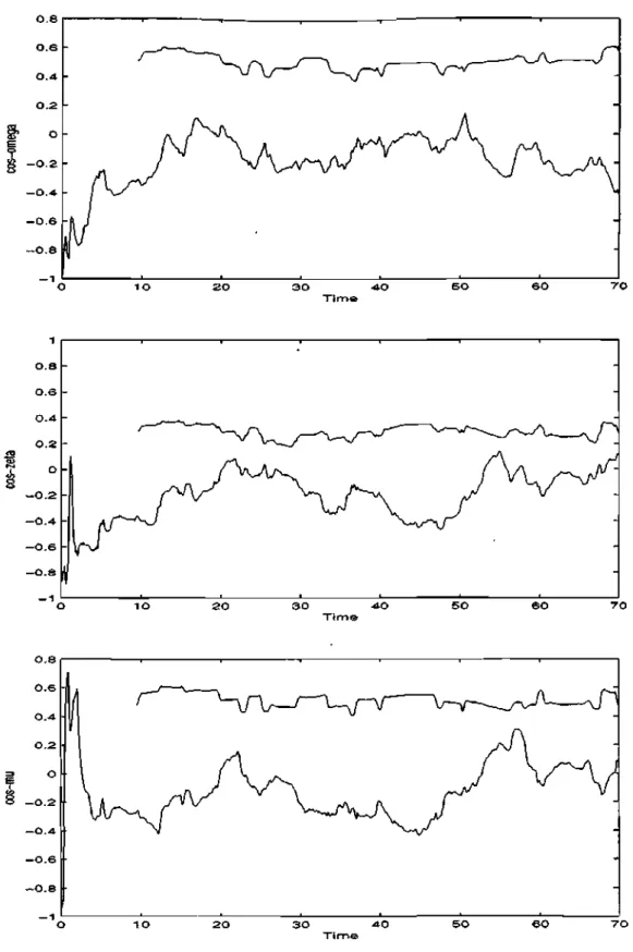
Figure 2 shows the behavior of cosines for a;, £ and \x. Note again that the compu-tations have only meaning after t = T = 10 (selected window size for inner product). Although none of the cosines has shot the alarm, the cosines corresponding to ( and

(i have been close to alarm activation. In fact, for M = 1 both cosines do cross the

boundary. In general, this cosine-based scheme is also quite sensitive to additive faults which may not come from parametric changes; on the other hand, they may generate frequent false alarms when system noise increases.

5.4 Parameter changes

Changes in the values of u, C and y. have been considered separately (all changes are applied at To = 45):

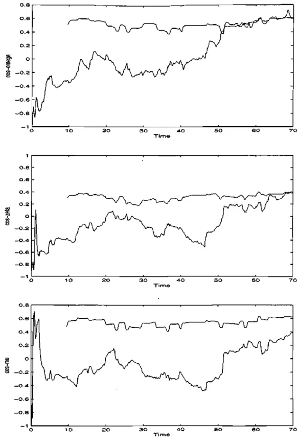
1. Variation so that LJ = 2 (i.e., 6u = 1). The cosine corresponding to v^ crosses the boundary at detection time Td ~ 52. No other cosine alarm is shot until t approaching 70 (cosine of <pw) but it does so in a very small slot of time.

es are

C 8 h

0 . 6 h

0.4- h

- 0 . 2 h

- 0 . 4

O . I 5

O . I

\-0 . \-0 5 h

- O . I

7 0

3 0 -40 T i m e

5 0 7 0

rosses

mtil t Figure 1: Mean estimators for parameter variation Su = 1.

Figure 2: Cosines for parameter variation 8u = 1.

2. Variation with S( = 1. The cosine corresponding to (p^ crosses the boundary at detection time T& « 52. No other cosine alarm is shot until t approaching 60

(cosine of p^) but it does so in a very small slot of time.

3. Variation with 5/j, = 1. No alarm is shot. When 8(j, approaches 1.5 two alarms are activated: cosine corresponding to <p^ and cosine corresponding to (pc..

Figure 3 shows the results for the evolution of the three cosines when Su) = 1.

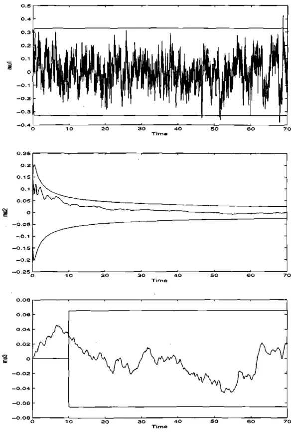
Concerning m detectors, in all the cases only p,\ crosses the boundary near to £ = 70 in a very small slot of time. This corresponds with the behavior of such estimator mentioned above. In general, these estimators are not very sensitive to parameter variations. Figure 4 shows the behavior for these mean estimators.

6 Concluding remarks

The analyzed existing fault detection schemes have presented very different properties concerning their sensitivity. On one hand, mean-estimation based detectors show a very robust behavior having few false alarms. Nevertheless they do not easily detect other types of failures which do not affect the mean. On the other hand, cosine-based estimators can detect different types of faults, but they are very sensitive to parameter tuning and system noise, presenting frequent false alarms. The analysis suggests the use of a combined scheme, which could be supervised by a high level decision rule set.

Acknowledgements

This work has been partially supported by project MTM2007-62064 of the Plan Na-tional de I+D+i, MEyC, Spain, and by project CCG07-UPM/000-3278 of the Univer-sidad Politecnica de Madrid (UPM) and CAM, Spain.

References

[1] E. ALCORTA-GARCIA AND P. M. FRANK, Deterministic nonlinear observer-based approaches to fault diagnosis: a survey, IFAC Control Engineering Practice 5

(1997) 663-670.

[2] M. BASSEVILLE AND I. V. NIKIFOROV, Detection of Abrupt Changes. Theory and

application, Prentice Hall, 1993.

[3] A. CASTILLO, P . ZUFIRIA, M. M. POLYCARPOU, F. PREVIDI, AND T. PARISINI,

Fault detection and isolation scheme in continuous time nonlinear stochastic sys-tems., Proceedings of the 5th IFAC Symposium on Fault Detection, Supervision

and Safety of Technical Processes SAFEPROCESS 2003 (2003) 651-656.

TO 2 0 3 0 4 0 5 0 SO T i m e

3

rl

T i m e

7 0

Figure 3: Cosines for parameter variation 5UJ = 1.

r o

3 0 4 0 T i m ©

5 0 6 0

o.oa

0 . 0 2

Figure 4: Mean estimators for parameter variation 8LU — 1.

[4] A. CASTILLO, Fault Detection and Isolation via Continuous Time Statistics, rm

Ph.D. Thesis, E.T.S. Ingenieros Industrials (Universidad Politcnica de Madrid) (2006).

[5] C. D E PERSIS AND A. ISIDORI, A Geometric Approach to Nonlinear Fault

Detec-tion and IsolaDetec-tion, IEEE Trans. Automat Control 46 (2001) 853-865.

[6] P. M. FRANK, Analytical and qualitative model-based fault diagnosis-A survey and

some new results, Eur. J. Contr. 11 no. 2 (1996) 26-28.

[7] J. J. GERTLER, Fault Detection and Diagnosis in Engineering Systems, Marcel Dekker, New York, 1998.

[8] R. ISERMAN, Fault-Diagnosis Systems. An introduction to fault detection and fault

tolerance, Springer Verlag, 2006.

[9] U. MNZ AND P. ZUFIRIA, Parametric Fault Diagnosis in Stochastic Dynamical

Systems, Proceedings of the 19th CEDYA. Madrid, Spain. (2005)

[10] U. MUNZ AND P . ZUFIRIA, Diagnosis of unknown parametric faults in non-linear stochastic dynamical systems, Int. J. of Control (2008) In Press.

[11] M. M. POLYCARPOU AND A. T. VEMURI, Learning Methodology for Failure

De-tection and Accomodation, IEEE Control Systems (1995) 16-24.

[12] M.M. POLYCARPOU AND A. B. TRUNOV, Learning approach to nonlinear fault

diagnosis: Detectabihty analysis, IEEE Tr. Aut. Contr. 45 (2000) 806-812.

[13] X. ZHANG, M . M . POLYCARPOU AND T. PARISINI, A Robust Detection and

Iso-lation Scheme for Abrupt and Incipient Faults in Nonlinear Systems, IEEE Tr.

Aut. Contr. 47 (2002) 576-593.

[14] X. ZHANG, T. PARISINI AND M . M . POLYCARPOU, Sensor Bias Fault Isolation

in a Class of Nonlinear Systems, IEEE Tr. Aut. Contr. 50 NO. 3 (2005) 370-376.