Bayesian network modeling of the consensus between experts: an application to neuron classification

(1)

Bayesian network modeling of the consensus between experts: An a

pplicatio

n

to neuron classification

Pedro L. López-Cruz a, , Pedro Larrañaga a, Javier DeFelipe b, Concha Bielza a

a Computational Intelligence Group, Departamento de Inteligencia Artificial, Facultad de Informática, Universidad Politécnica de Madrid, Campus de Montegancedo sn, 28660 Boadilla del Monte, Madrid, Spain

b Instituto Cajal (CSIC) and Laboratorio de Circuitos Corticales (Centro de Tecnología Biomédica), Universidad Politécnica de Madrid, Spain

ABSTRACT

Neuronal morphology is hugely variable across brain regions and species, and their classifi-cation strategies are a matter of intense debate in neuroscience. GABAergic cortical interneu-rons have been a challenge because it is difficult to find a set of morphological properties which clearly define neuronal types. A group of 48 neuroscience experts around the world were asked to classify a set of 320 cortical GABAergic interneurons according to the main fea-tures of their three-dimensional morphological reconstructions. A

methodology for building a model which captures the opinions of all the experts was proposed. First, one Bayesian network was learned for each expert, and we proposed an algorithm for clustering Bayesian networks corresponding to experts with similar behaviors. Then, a Bayesian network which represents the opinions of each group of experts was induced. Finally, a consensus Bayesian multinet which models the opinions of the whole group of experts was built. A thorough analysis of the consensus model identified different behaviors between the experts when classifying the interneurons in the experiment. A set of characterizing morphological traits for the neuronal types was defined by performing inference in the Bayesian multinet. These findings were used to validate the model and to gain some insights into neuron morphology. © 2013 Elsevier Inc. All rights reserved.

1. Introduction

The morphologies, molecular features and electrophysiological properties of neuronal cells are extremely variable [1–4]. Neuronal morphology is a key feature in the study of brain circuits, as it is highly related to information process-ing and functional identification. Except for some special cases, this variability makes it hard to find a set of features that unambiguously define a neuronal type [3]. In addition, there are distinct types of neurons in particular regions of the brain. Indeed, neurons in the cerebral cortex can be classified into two main categories based on their morphology: pyramidal neurons and interneurons (Fig. 1). In general, pyramidal neurons are excitatory (glutamatergic) cells which display spines in their dendrites and have an axon which projects out of the white matter. Their name refers to the pyramidal shape of their soma. Interneurons are cells with short axons that do not leave the white matter and their dendrites show few or no spines. These interneurons appear to be mostly GABAergic (inhibitory) and constitute 15–30% of the total neuron population, but they display chemical, physiological and synaptic heterogeneity [3]. Thus, the identification of classes and subclasses of interneurons is clearly critical for gaining a better understanding of how these cell shapes relate to cortical functions in both health and disease. This paper focuses on GABAergic interneurons, which also show a remarkable morphological variability between species, layers and areas [5]. The Internet has made it possible for researchers to share digital three-dimensional reconstructions of neuronal morphology in publicly accessible databases [6,7]. With such amount of available data, a

com-Corresponding author.

E-mail addresses: [email protected] (P.L. López-Cruz), [email protected] (P. Larrañaga), [email protected] (J. DeFelipe), [email protected]

(2)

Fig. 1. Photomicrograph from Cajal’s preparation of the occipital pole of a cat stained with the Golgi method, showing a pyramidal cell (one arrow) and an interneuron (neurogliaform cell) (two arrows). From DeFelipe and Jones (Cajal on the Cerebral Cortex, Oxford University Press, New York, 1988).

mon nomenclature for naming cortical neuronsisacrucial prerequisite for advancinginour knowledgeofneuronal structure [3,8].

Bayesian networks [9,10] are a kind of probabilistic graphical model that provides a natural way of modeling uncertainty in artificial intelligence. Therefore, they have been successfully applied across a large number of problems from very different domains [11 ]. Bayesian networks are specially well suited for modeling and incorporating expert’s knowledge, although this kind of analysis has not been applied to its full potential for neuron classification. There are two approaches for integrating this information into a Bayesian network. First, we can elicit both the structure [12] and the parameters [13] of the Bayesian network. Second, we can build a dataset which reflects the behavior of the expert and learn a Bayesian network from the data. This paper focuses on the second approach, i.e., a consensus Bayesian network is built based on data which reflects expert opinions.

We present a methodology for building a Bayesian network that models the opinions of a group of experts. First, a Bayesian network was learned for each expert, representing his/her behavior in the classification task. Second, a clustering algorithm was run on the Bayesian networks to find groups of experts with similar behaviors, and a representative Bayesian network was induced for each cluster of experts. Expert behavior when classifying the set of interneurons was extremely variable. Therefore, experts with similar behaviors have to first be clustered and then combined. Otherwise, combining all experts behaviors into a single consensus model would presumably hide some of these differing behaviors [14,15]. In this way, we can explicitly model each group of similar experts as a representative Bayesian network for the cluster. Third, the final consensus model wasa Bayesian multinet [16] encoding amixtureof Bayesian networks [17 ,18], where each component was the Bayesian network which represented the opinions of a cluster of experts. A similar idea has been proposed for case-based Bayesian networks [19 ,20], where the authors cluster the observations before learning a Bayesian network which captures the different properties of each cluster. Bayesian multinets are a kind of asymmetric Bayesian network which allows to model different statistical (in)dependences between the variables for different values of a distinguished variable. Bayesian multinets can capture local differences between variables and model the problem domain more closely, allowing for sparser models and more robust parameter estimation. For instance, they have been shown to outperform other Bayesian network models in supervised classification problems [21].

(3)

W e apply t h e p r o p o s e d m e t h o d o l o g y t o t h e p r o b l e m of t h e morphological classification of GABAergic i n t e r n e u r o n s from t h e cerebral cortex. The research is based o n a previous study [22], w h e r e w e selected a n d asked a g r o u p of 4 8 e x p e r t s t o classify a set of 3 2 0 i n t e r n e u r o n s according t o their m o s t p r o m i n e n t morphological features. However, t h e methodology p r e s e n t e d in this study can b e applied t o a w i d e range of scientific fields. For instance, in a medical setting, it m a y b e interesting t o m o d e l a n d analyze t h e different opinions of a g r o u p of physicians regarding t h e diagnosis, prognosis or t h e m o s t a p p r o p r i a t e t r e a t m e n t for a given disease. Another e x a m p l e c a n b e found in a risk a s s e s s m e n t scenario, w h e r e different people could have different opinions o n a given m a t t e r d e p e n d i n g o n their personal preferences, risk perception, etc. The process of obtaining t h e opinions of different e x p e r t s o n a given task (here, t h e morphological classification of i n t e r n e u r o n s ) is challenging because it can b e difficult, costly a n d t i m e c o n s u m i n g . However, n e w Internet tools a n d c r o w d -sourcing t e c h n i q u e s have alleviated s o m e of t h e s e problems, a n d obtaining classification d a t a from different e x p e r t s is n o w affordable for a lot of p r o b l e m s [23].

The p a p e r is organized as follows. Section 2 explains t h e d a t a acquisition process for gathering t h e experts’ morphological classification of t h e set of i n t e r n e u r o n s . Section 3 details t h e p r o p o s e d m e t h o d o l o g y for building a c o n s e n s u s Bayesian m u l t i n e t w h i c h m o d e l s experts’ opinions. Section 4 includes t h e evaluation of t h e m o d e l a n d t h e biological interpretation of t h e results. Finally, Section 5 e n d s w i t h conclusions a n d suggestions for future w o r k .

2. Interneuron classification by a set of experts

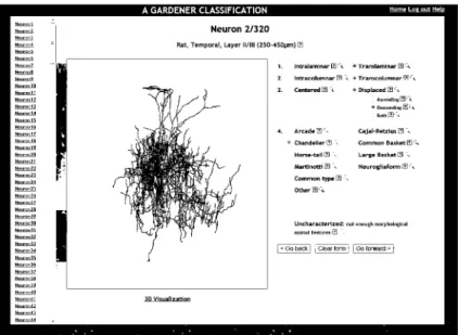
We selected N = 3 2 0 cortical GABAergic i n t e r n e u r o n s from different s p e c i e s : cat, h u m a n , monkey, m o u s e , rabbit a n d rat u s e d in a previous s t u d y [22]. Briefly, t h r e e - d i m e n s i o n a l reconstructions of 2 4 1 of t h o s e i n t e r n e u r o n s w e r e retrieved from NeuroMorpho.org [7], w h e r e a s t h e rest w e r e s c a n n e d from relatively old p a p e r s w i t h n o d a t a on t h e t h r e e - d i m e n s i o n a l distribution of their d e n d r i t e s a n d axons. A set of 4 8 e x p e r t s w e r e asked t o classify each o n e of t h e n e u r o n s according t o their m o s t p r o m i n e n t morphological features. A w e b a p p l i c a t i o n1 w a s built t o display t h e n e u r o n a l m o r p h o l o g i e s for t h e participants a n d t o retrieve their classifications. Two-dimensional projections of all t h e n e u r o n s w e r e available. Additionally, a t h r e e - d i m e n s i o n a l visualization a p p l e t b a s e d o n Cvapp software [24] w a s provided for t h e n e u r o n s t a k e n from NeuroMor-pho.org, w h i c h experts could u s e t o navigate, rotate a n d z o o m t h e n e u r o n a l morphologies. Fig. 2 s h o w s a screenshot of t h e w e b application. Additional d a t a a b o u t t h e location of t h e n e u r o n , such a s t h e cortical area, t h e layer a n d t h e thickness of t h e layer w e r e included w h e n available. Other w e b application features included a h e l p page w i t h instructions a n d defini tions of t h e n e u r o n a l types, a n d a search engine w h i c h s h o w e d o t h e r n e u r o n s previously classified by t h e e x p e r t a s a given n e u r o n a l t y p e . These d a t a w e r e o b t a i n e d a n d analyzed in [22]. The goal of this research w a s t o achieve a c o m m o n n o m e n clature for t h e cortical GABAergic i n t e r n e u r o n s w i t h a utilitarian p u r p o s e . The a g r e e m e n t b e t w e e n e x p e r t s w h e n classifying t h e i n t e r n e u r o n s w a s studied at length. W e found t h a t a g r e e m e n t w a s reasonably high for t h e a t t r i b u t e s describing t h e general n e u r o n a l morphology. Looking at t h e low-level classification i n t o t e n different n e u r o n a l types, however, w e found remarkable d i s a g r e e m e n t s b e t w e e n t h e e x p e r t s for s o m e n e u r o n a l t y p e s . Here, t h e goal is t o build a c o n s e n s u s Bayesian m u l t i n e t w h i c h m o d e l s t h e opinions of all t h e experts a n d t o u s e this m o d e l t o further investigate their a g r e e m e n t s a n d d i s a g r e e m e n t s .

The e x p e r t s w h o participated in t h e e x p e r i m e n t w e r e asked t o classify t h e n e u r o n s according t o four a t t r i b u t e s describing t h e m a i n morphological features of t h e n e u r o n s :

1. The first a t t r i b u t e described t h e horizontal distribution of t h e axon relative t o t h e cortical layer. Here, t h e e x p e r t s h a d t o s e p a r a t e n e u r o n s w i t h a n axonal arborization in t h e s a m e layer a s t h e s o m a (Intralaminar) from n e u r o n s w i t h axons distributed in different layers (Translaminar).

2. The second a t t r i b u t e referred t o t h e vertical distribution of t h e axon relative t o a reference cortical c o l u m n ( w i d t h = 3 0 0 μm). The e x p e r t s h a d t o classify each n e u r o n according t o w h e t h e r t h e axonal arborization is distributed primarily in t h e s a m e cortical c o l u m n (Intracolumnar) or in different cortical c o l u m n s (Transcolumnar).

3 . The t h i r d a t t r i b u t e r e p r e s e n t e d t h e relative position of t h e axon a n d t h e d e n d r i t e s . N e u r o n s w i t h d e n d r i t i c a r b o r s placed i n t h e c e n t e r of t h e axonal arborization w e r e classified a s Centered, w h e r e a s n e u r o n s w i t h d e n d r i t e s shifted w i t h respect t o t h e axon w e r e classified a s Displaced. W h e n a n e u r o n w a s classified a s b o t h Translaminar a n d Displaced, t h e e x p e r t s w e r e asked t o further characterize t h e n e u r o n s according t o w h e t h e r t h e axon w a s directed t o w a r d s t h e cortical surface (Ascending), t h e w h i t e surface (Descending) or b o t h (Both).

4 . The fourth a t t r i b u t e included a low-level classification of t h e n e u r o n s i n t o n i n e n e u r o n a l t y p e s w h i c h a r e frequently u s e d i n t h e literature [2 5] : Arcade, Cajal-Retzius, Chandelier, Common basket, Horse-tail, Large basket, Martinotti, Neurogliaform a n d Common type. Additionally, t h e e x p e r t s could classify a n e u r o n as Other a n d provide a n alternative n a m e for t h a t n e u r o n if t h e y felt t h a t it d i d n o t fit any of t h e p r o p o s e d n e u r o n a l t y p e s .

A n e u r o n w a s classed a s Uncharacterized w h e n t h e reconstructed p a r t of t h e m o r p h o l o g y w a s n o t clear e n o u g h ( d u e t o incomplete labeling, reconstruction noise, etc.) for it t o b e w o r t h w h i l e having a go at classification. W h e n a n e u r o n w a s classified a s Uncharacterized, n o value could b e given for t h e o t h e r a t t r i b u t e s .

(4)

Fig. 2. Web application showing one of the 320 neurons to be classified by each expert.

Each expert was administered the form in Fig. 2 for each neuron. When the experiment finished, 42 out of the 48 experts had classified all 320 neurons. We only used the information about the 42 experts who completed the experiment. The goal in this paper was to build a model which encoded the opinions of the experts when classifying the interneurons in the experiment.

3. A methodology for inducing a consensus Bayesian multinet from a set of expert opinions

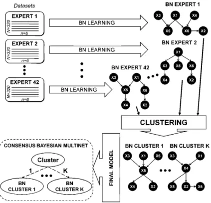
In this section, we detail the process for obtaining a Bayesian multinet representing the consensus among the experts who completed the experiment. Fig. 3 visually represents the whole methodology, which can be summarized in three main steps:

1. Learn one Bayesian network for each expert using the classifications provided in the experiment.

2. Cluster the Bayesian networks into groups and induce a new representative Bayesian network for each cluster, which models the opinions of the experts in the cluster.

3. Combine the representative Bayesian networks of each cluster into one consensus Bayesian multinet.

The following sections describe each step in the previous methodology. Section 3.1 introduces Bayesian networks theory and details how to use the classification provided by each expert to learn a Bayesian network representing his/her behavior in the experiment. Section 3.2 explains how to discover groups of similar Bayesian networks by applying clustering algorithms and how to induce a representative Bayesian network for each group. In Section 3.3, the final consensus Bayesian multinet model is built from the representative Bayesian networks of each cluster.

3.1. Bayesian network modeling of each expert’s behavior

Bayesian networks [9,10] are a class of probabilistic graphical models, defined as a pairB = (G(X, A), P), where:

• G(X, A) is the graphical component of the model, i.e., a directed acyclic graph (DAG) where the nodes (X) represent the variablesX = {X1,...,Xn] in the problem domain and the arcs (A) encode the probabilistic conditional (in)dependence relationships between the variables.

• P is the probabilistic component of the model. P includes a conditional probability table P(Xi|Pa(Xi)) for each variable

Xi, i = 1, ..., n in the problem, where Pa(Xi) is the set of parents ofXi in G: Pa(Xi) = [Y e X|(Y,Xi) e A}. Therefore, P = {P(Xi|Pa(Xi), i = 1 , . . . , n}.

A Bayesian network encodes a factorization of the joint probability distribution (JPD) over all the variables inX:

P(X) = P[P(Xi|Pa(Xi)). (1)

(5)

Fig. 3. General methodology for building a consensus Bayesian multinet which represents the behavior of a set of experts.

Bayesian networks are both interpretable and efficient. The graphical component of a Bayesian network is a compact representation of the problem domain, while the factorization of the JPD reduces the computational workload of using high-dimensional probability distributions.

Bayesian network learning from data is a two-step procedure [26–28]: structural search and parameter fitting. There are two main methods for learning the structure G of aBayesian network: constraint-based methods and score+search methods. Constraint-based methods rely on performing statistical tests to find conditional independence relationships between groups of variables in the network. Then, an undirected independence graph is built, and edge orientation discovers a Bayesian network structure which encodes those conditional independence relationships. Score+search approaches use a heuristic search algorithm to explore the space of DAGs, and a score function to evaluate the candidate network structures and direct the search procedure. Once the network structure has been found, the parameters in the conditional probability tables (P) are estimated from the counts in the dataset.

We focused on score+search methods and learned the Bayesian network structure using the greedy thick thinning (GTT) algorithm [29] implemented in the GeNIe free modeling environment.2 K2 scoring function [30] was used to evaluate each candidate structure, by measuring the joint probability of the Bayesian network structure G and a dataset D:

n <jj

n

(r; — 1)! JL

_1 j-1 ( Ny + n — 1 )! £1

(2)

where P(C) is the prior probability of the network structure G, r; is the number of distinct values of X;, <j; is the number of possible configurations ofPa ( X;) ,N,j is the number of instances in the dataset D where the set of parents Pa ( X;) takes their j-th configuration, and Np is the number of instances where the variable X; takes the fc-th value X& and Pa(X;) takes their j-th configuration (Ny = Y?k=1 Np).

The GTT algorithm implements a two-step procedure for discovering a Bayesian network structure (see Algorithm 1). Given an initial (empty) graph G, it iteratively adds the arc which maximizes the increase in the likelihood (thicking step). When no further increment is possible by adding arcs, the algorithm iteratively removes arcs until no arc deletion yields a positive increase in the likelihood (thinning step). Then, the algorithm stops and the resulting Bayesian network structure is returned. The GTT algorithm has a number of advantages, e.g., unlike other methods [30-32] it does not require an ordering of the variables. Also, it is simple, computationally efficient and avoids overfitting by removing arcs in the thinning step.

(6)

Algorithm 1 (Greedy thick thinning algorithm).

(, )

Given a n initial graph G X A a n d a d a t a s e t D

1. Thicking step: While the K2 score function (2) increases:

(a) Find the arc ( X;, Xj ) which maximizes (2) when included in G'( X , A') with A' = A U {( X;, Xj )}. (b) Set G <r- C'.

2. Thinning step: While the K2 score function (2) increases:

(a) Find the arc ( X;, Xj ) which maximizes (2) when deleted in G'( X , A') with A' = A \ {( X;, Xj )}. (b) Set G <r- C'.

3. Return G.

A Bayesian network was learned for each one of the Ne = 42 experts who completed the experiment. The goal was to build

a model which captures how each expert understands the values of the morphological attributes and their relationships. The graphical representation of the Bayesian networks structures offers a compact and easy way for the experts in the domain to interpret their models. The Bayesian networks were learned independently for each expert, so they do not capture whether or not the experts classified the same neurons in the same way. However, since the experts classified the same set of interneurons, we can use the Bayesian networks to systematically analyze their opinions and behaviors. One would expect that if two experts differed in their opinions (as encoded in their Bayesian networks), then they would also classify the neurons differently. Also, having an individual Bayesian network for each expert makes it easier to analyze and validate the representative Bayesian networks for each cluster and the final consensus Bayesian multinet, because the inputs (Bayesian networks) and the output (Bayesian multinet) share the same representation.

Therefore, one dataset for each expert was generated with the classifications provided in the experiment. The resulting datasethadN = 320 observations (the number of interneurons in the experiment) and n = 6 variables, which corresponded to the features that the experts were asked to classify. Some restrictions on different combinations of feature values were imposed in the experiment design (see Section 2). For instance, selecting Uncharacterized in the first feature disabled all the other variables. Therefore, when a neuron was classified as Uncharacterized, the values for the other variables were empty. Similarly, t h e Ascending/Descending/Both feature w a s only available w h e n Translaminar and Displaced were selected for the corresponding features. To build the dataset for each expert, we filled in incomplete observations with a new category named Dummy. Therefore, for each expert, we had a dataset with n = 6 categorical variables with values:

• X1 (j1 = 2): Characterized, Uncharacterized. • X2 (r2 = 3 ) : Intralaminar, Translaminar, Dummy. • X3 (r3 = 3 ) : Intracolumnar, Transcolumnar, Dummy. • X4 (V4 = 3 ) : Centered, Displaced, Dummy.

• X5 (r5 = 4 ) : Ascending, Descending, Both, Dummy.

• X6 (r6 = 11): Common type, Horse-tail, Chandelier, Martinotti, Common basket, Arcade, Large basket, Cajal-Retzius,Neurogliaform, Other, Dummy.

We used the data provided by each expert in the experiment to learn a Bayesian network which encoded the conditional independence relationships between the variables for that expert. The GTT algorithm was used to find the Bayesian network structure, and the parameters were fitted using maximum likelihood estimators with Laplace correction. We did not allow any variable to be a parent of variable X1, corresponding to the Characterized/Uncharacterized feature. This restriction encoded the knowledge that the decision of classifying a neuron as Characterized or Uncharacterized should be taken before classifying all the other features (modeled with variablesX2toX6). We limited the complexity of the Bayesian networks by imposing a maximum of three parents for each variable. This allowed us to control the size of the conditional probability distributions and to compute robust estimators of their parameters. However, this was not a very restrictive constraint since only 5 out of 6 x 42 = 252 variables in all the Bayesian networks had three parents.

(7)

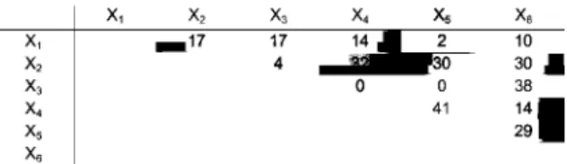
Fig. 4. Number of Bayesian networks including the edge for each pair of variables. The matrix is symmetric so only the upper triangle is shown. Light-shaded cells show agreements in the experts’ Bayesian network structures, i.e., edges which appear in most or none of the Bayesian networks, whereas dark-shaded cells show disagreements in the Bayesian network structures.

3.2. Clustering of Bayesian networks

The experiment was designed to find groups of Bayesian networks corresponding to experts with similar behaviors. In this section, we detail the process of finding groups of Bayesian networks which define similar JPDs and inducing a representative Bayesian network for each cluster. To the best of our knowledge, the problem of clustering Bayesian networks had not been studied before. Note that this is not the same problem as using Bayesian networks to cluster data [33,34] or clustering variables in Bayesian network learning for high-dimensional problems [35,36]. Bayesian networks have two main components (see Section 3.1): the graphical part and the probabilistic part. Therefore, we could consider clustering at the two levels:

• Clustering of Bayesian network structures: The graphical component G(X, A) of a Bayesian network is a DAG which

encodes the conditional (in)dependence relationships between the variables in the problem domain. Therefore, we could use existing approaches for clustering graphs [37,38] and, in particular, clustering DAGs [39] to find groups of structurally similar Bayesian networks. Another approach could be to list the conditional independence relationships encoded in a Bayesian network and then apply a clustering algorithm to group Bayesian networks which share the same set of conditional independences.

• Clustering of Bayesian network probabilities: The probabilistic component P in a Bayesian network contains the

condi-tional probability distributions of each variable Xi given its parents Pa(Xi). Clustering of probability distributions has not received much attention in the statistics and machine learning fields. The approaches in [40,41 ] cannot be directly applied to our problem because P includes several (conditional) probability distributions: one probability distribution for each variable given its parents’ values. Comparing the conditional probability distributions of the same variable in two different Bayesian networks is challenging because each variable can have a different number of parents, and the set of parents may be different. Therefore, the conditional probability distributions cannot be directly compared. A simple approach, which could also be useful in problem domains with a lot of variables, would be to compute the marginal probability distribution for each variable in each Bayesian network and to cluster the Bayesian networks based on these marginal distributions.

Here, we propose clustering the Bayesian networks based on the joint probability distributions that they encode. There-fore, our approach is included in the second group of techniques. Fig. 5 outlines the proposed methodology, which can be summarized in three steps. First, the JPD encoded by each Bayesian network is computed. These JPDs also model the experts’ behavior in the experiment. Second, groups of similar experts/Bayesian networks are found by clustering their correspond-ingJPDs. Third, a representative Bayesian network is induced for each cluster, which represents the common behavior of the experts in the cluster. The following sections detail each one of these three steps.

3.2.1. Computation and preprocessing of the joint probability distributions

For each expert, we computed the JPD over the six variables encoded by the Bayesian network learned in the previous step. Not all the experts selected all the possible values when completing the experiment, e.g., some experts did not classify any neuron as Arcade, Cajal-Retzius or Other in variable X6. Therefore, not all the Bayesian networks contained all the values for all the variables. However, we wanted all the JPDs to have the same number of values for the purposes of comparison. Therefore, we completed the conditional probability tables in the Bayesian networks learned with GeNIe using maximum likelihood estimators with Laplace correction, so that all the Bayesian networks had all the values for all the variables. Then, the JPD over all the variables encoded by each Bayesian network was computed by multiplying the conditional probability distributions in P, as in Eq. (1). The resulting JPD had 2x 3x3x 3x4x1 1 = 2376 values. However, most of these values corresponded to inadmissible combinations of the values of the variables. For example, when Uncharacterized was selected, all the other variables should have the value Dummy and any other combination of values was not valid. Similarly, variable X5 could only take a value different from Dummy when X2 = Translaminar and X4 = Displaced. We erased the values in the JPDs corresponding to these forbidden combinations. The resulting JPDs had 121 values each.

3.2.2. Clustering of joint probability distributions

(8)

Fig. 5. Procedure for clustering Bayesian networks. In step 3, the solid line represents the proposed workflow for inducing a representative Bayesian network for each cluster, whereas the dashed lines show alternative ways of achieving this goal.

was a JPD corresponding to the Bayesian network of each expert and each variable (column) was a value of the JPD. There are three main paradigms which can be used for clustering [42]: probabilistic, hierarchical and partitional clustering.

Hierarchical and partitional paradigms are the classical approaches to clustering. In general, both paradigms rely on the definition of a distance or dissimilarity measure between the observations. A classical agglomerative (bottom-up) hierarchical clustering algorithm starts with one cluster per observation and iteratively merges the two most similar clusters according to some criterion, called linkage function, which depends on the distances of the observations in the clusters. Therefore, hierarchical clustering techniques do not generate a single partition but a hierarchy of clusters. On the contrary, partitional clustering techniques generate a single partition of the objects into clusters by applying an optimization process which maximizes/minimizes an objective function. This objective function usually measures the distances between the objects in the same cluster (minimization) and/or the distance between objects in different clusters (maximization). In both hierarchical and partitional approaches, the number of clusters to be generated is a free parameter that has to be set by the expert. Also, an appropriate distance measure has to be chosen depending on the nature of the data.

Probabilistic clustering deals with the problem of fitting a finite mixture of distributions [43], where each component is the probability distribution which models the observations belonging to the cluster. Probabilistic clustering offers a number of advantages. First, it generates a probabilistic model which describes the data. Using that model, one can compute the (posterior) probability of a given observation belonging to each cluster. Also, it is able to formally address the problem of model selection (finding an appropriate number of clusters). Since each of our observations is aJPD, the Dirichlet distribution [44] could be a suitable choice of a probability density function for each component. However, the low number of observations (Ne = 42) over the number of variables (r = 121) ruled out the use of this approach, because it is difficult to obtain accurate

estimators of a finite mixture model with so few data.

Here, we chose to adapt the classical IC-means algorithm [45] to characterize properties of our data. Algorithm 2 shows a general outline of the algorithm. The algorithm alternates two steps. First, the observations are assigned to the cluster with the closest center. Second, the cluster centers are recomputed taking into account only the observations in the clusters.

Algorithm 2 (K-means algorithm).

Input: the number of clusters K and a dataset of r-dimensional observations P = {o;,..., ojve}. Steps:

1. Initialize the cluster centers C = {c1,..., c^} to K random observations in P without replacement. 2. While the cluster centers C change

(a) For each observation o;, compute the dissimilarity between o; and each cluster center c^: d(o;, c&).

(9)

The K-means algorithm iteratively minimizes the sum of the distances of each observation to its cluster center:J(P, C) = X;=1 d (oj, ck* J. K-means is guaranteed to find a local minimum of/(P, C). Therefore, Algorithm 2 is usually restarted several times with different initialization values for step 1. A similar approach was used in [14,15] in the context of decision making in influence diagrams. In order to apply the K-means algorithm to the problem of clustering JPDs we have to choose a suitable dissimilarity measure d(o;, c&) and a method for computing the cluster centers from the observations in the cluster

(Combine function in step 2(c) of Algorithm 2).

Dissimilarity measures for probability distributions. In general, our choice of a dissimilarity measure d(o;, c&) should be, at

least, symmetric. Therefore, one could consider using the symmetric Kullback-Leibler divergence,

d/aCp1, p2) = KL(p1||p2) + Kl(p21|p1),

where KI(p1||p2) is the Kullback-Leibler divergence [46] from an empirical probability distribution p1 to the true distribution p2

r

Kl( p1 || p2 )= p1jlog—,

1=1 2

where r is the number of values of the probability distribution p;, and py is the probability of the jth value in the probability distribution p;. One disadvantage of the Kullback-Leibler divergence is that it is not upper bounded. However, other measures can be considered, such as the Jensen-Shanon divergence,

1 1

drc(p1,p2) = -Kl(p1||m)H—Kl(p2||m), (3)

2 2

where m is the mean probability distribution m = 0.5 (p1 + p2). The Jensen-Shanon divergence has a number of interesting properties [47]: it is symmetric, its square root is a metric and it is bounded 0 < djs < 1. Therefore, we chose djs as the dissimilarity measure for the K-means algorithm. Additionally, the fact that djs is a bounded measure was also useful when computing the representative Bayesian network for each cluster (Section 3.2.3).

Combination of probability distributions. Two main methods can be found in the literature to compute an average

prob-ability distribution p from a set of probprob-ability distributions [48]: the linear combination pool (LinOp) and the logarithmic combination pool (LogOp). If we have N& probability distributions { p 1 , . . . , p^t} in a cluster, the linear combination pool is

defined as the weighted arithmetic mean

ptinOp = vp, (4)

i=1

where X ; i1 &>i = 1and&>; > 0 is the weight for the probability distribution p;. The logarithmic combination pool is defined as the weighted geometric mean

uN k rf0'

PjLogOp = —Hk ^ 7 - (5)

2-*v=1 Hi = 1 Piv

Genest and Zideck [48] give a number of reasons for choosing LogOp over LinOp, the most compelling being that it is externally Bayesian, i.e., it can be derived from joint probabilities [49]. Also, it is known that LinOp does not preserve independences [50], i.e., combining probability distributions which share a common independence does not guarantee that the resulting distribution will be equally independent. Heskes [51] showed that using LogOp is equivalent to finding the probability distribution p which minimizes the weighted sum of the Kullback-Leibler divergences to each probability distribution pj

piogPp = argmin ^&>;KL ( p || pi ) .

p i=1

Therefore, we chose LogOp as a combination method for computing the cluster centers in the K-means algorithm (step 2(c) of Algorithm 2). All the experts were considered as equals, so the weights &>; were all set to 1/N& for each cluster.

3.2.3. Finding a representative Bayesian network for each cluster

Once the JPDs have been clustered and K cluster centers (JPDs) have been obtained, the next step is to induce a Bayesian network which represents the common features of the corresponding Bayesian networks (and experts) in the cluster. Step 3 in Fig. 5 shows four possible approaches for finding a representative Bayesian network for each cluster. In the follow-ing, we discuss the four approaches for performing this task, we review the works related to each one and analyze their advantages and disadvantages for modeling experts’ opinions on the problem of the morphological classification of GABAer-gic interneurons.

(10)

to preserve that structure. They proposed a methodology for combining both the Bayesian network structures and the parameters. The algorithm finds a common network structure by transforming the DAGs into moral graphs, performing the union of the edges and transforming the resulting moral graph back into a DAG. The conditional probability tables are combined by applying the LogOp combination pool of Eq. (5). This approach is expected to yield highly connected Bayesian networks because of the union of the edges of the moral graphs. Therefore, the conditional probability distributions will have a lot of parameters and their estimates will not very robust when there are few training instances (in our scenario, 320 neurons). Sagrado and Moral [53] studied the theoretical properties of Bayesian networks obtained by performing either the intersection or the union of the arcs of the network structures, and proposed ways for finding the consensus Bayesian network structure. However, they left the combination of the conditional probability tables as a matter for future research. Zhang et al. [54] built on the work by Sagrado and Moral [53] and proposed a score+search method for fusing the Bayesian network structures. However, they applied Bayesian inference not data to combine the parameters of the Bayesian networks and to compute the scores of the network structures. Peña [55] derived a correction of the algorithms proposed by Matzkevich and Abramson [56,57] for finding the consensus Bayesian network structure with a minimum number of parameters. It represents only the common independences appearing in all the Bayesian network structures. He outlined some ideas for combining the parameters of the Bayesian networks, but this issue was mainly left for future research. Finally, other methods for Bayesian network aggregation have been proposed in the context of model averaging (for a review, see Section 4.13 in [28]). These methods combine the probabilities inferred with a set of Bayesian networks but they do not obtain a single representative Bayesian network which models the opinions of a set of experts. In the neuron classification problem, obtaining the representative Bayesian network explicitly was important because the experts would like to analyze and interpret these models and not only their outputs.

The second approach deals with the problem of learning a consensus Bayesian network from data. Maynard-Reich and Chajewska [58] assumed that the differences between experts are the result of observing different subsets of data. This is related to the problem of learning Bayesian networks from distributed datasets, see e.g. [59]. In our experiment, however, all the experts classified the same 320 interneurons, so this assumption did not apply. Steps 3.2.1 and 3.2.2 show another possibility which conformed to our problem: joining the original datasets for each expert in the cluster and learning a Bayesian network from this cluster’s dataset. We could consider different degrees of membership of each expert to his cluster by only including a subset of interneurons from his dataset in the cluster’s dataset. However, there were some neuronal morphologies which did not appear frequently in the data. Therefore, this approach could erase some important information about the experts.

The third approach is based on sampling the JPDs and learning a Bayesian network from the generated data as explained in Section 3.1 (Fig. 5, steps 3.3.1 to 3.3.3). First, we compute a representative JPD for each cluster, then we sample the JPD to obtain a dataset and, finally, we learn a Bayesian network from that dataset. Again, one could consider using the LinOp (Eq. (4)) or the LogOp (Eq. (5)) combination pools for computing the representative JPD and different weights could be applied to each expert’s JPD. However, if the cluster center JPD does not accurately represent all the experts in the cluster, the resulting representative Bayesian network for the cluster would not model all the experts’ opinions either.

Here, we implemented another approach based on proportional sampling of the individual JPDs of each expert (Fig. 5, steps 3.4.1 and 3.4.2). The goal was to obtain a sample of data for each cluster k, taking into account the dissimilarity between each JPD and the cluster center c& to decide the number of samples to draw from each JPD. The fact that dp(pi, c&) (Eq. (3)) is upper bounded facilitates the computation of these expert degrees of membership. For a given cluster k, we found the JPDs included in the cluster and computed a degree of membership /z; for each one as

1 — djs(pi, c&)

IM = K i •

zlj=1 (1 — djs(pj, cfc)J

Then, to obtain a sample with size M for cluster k, /x; x M observations were drawn from each JPD p; in cluster k. Finally, both the structure and the parameters of the representative Bayesian network were learned (Section 3.1) from that sample of size M obtained for each cluster.

This approach tries to avoid some of the disadvantages of the other three approaches. The learning algorithm allows to fully specify the Bayesian networks as opposed to the methods in the first approach (step 3.1.1), which can have problems when computing the parameters of the conditional probability distributions. An advantage of this method over the second approach (steps 3.2.1 and 3.2.2) is that our approach uses the Bayesian networks themselves (through their JPDs) to compute the representative Bayesian network for the cluster. The second approach, on the other hand, assumes that the Bayesian networks were learned from data and that experts’ data is still available. This may not be the case in some scenarios where Bayesian networks are elicited from experts’ knowledge and not induced from data. Finally, as opposed to the third approach, we consider each Bayesian network in the cluster individually through its JPD while taking into account different degrees of membership to the cluster.

3.3. Building the consensus Bayesian network

(11)

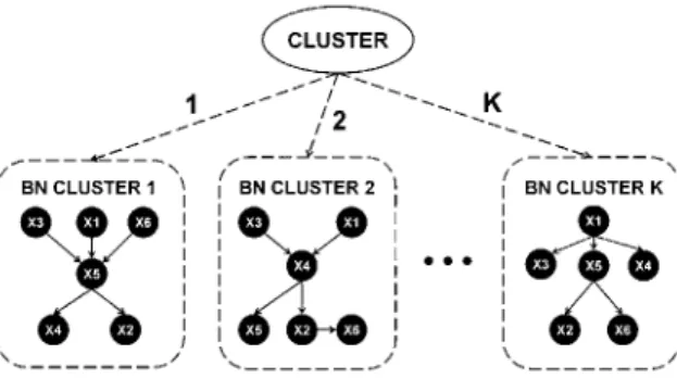
Fig. 6. Finite mixture of Bayesian networks represented as a Bayesian multinet with the cluster variable as the distinguished variable.

modeled the whole problem as a finite mixture of Bayesian networks [17] K

P(X = x) = TtkP{X = x\C = k, Gk, Pk), (6)

k=1

where jtk was set to the proportion of experts in the kth cluster (Nk/Ne), and each component P(X = x|C = k, Gk, Pk) was

the representative Bayesian network for the kth cluster with structural component Gk and probabilistic component Pk. Finite

mixtures of Bayesian networks form a kind of Bayesian multinet [16] with a distinguished variable C which represents the cluster variable. In principle, the cluster variable C is hidden but we found it previously by clustering the Bayesian networks (Section 3.2). Fig. 6 is a diagram of the final consensus Bayesian multinet.

4. Results

This section includes the results corresponding to one run of the whole process as described in Section 3 (see Fig. 3). First, one Bayesian network was learned for each one of the 42 experts who completed the experiment (Section 3.1). Then we clustered the Bayesian networks following the procedure described in Section 3.2. We started the process by computing theJPD encoded by each Bayesian network and generating a data matrix with dimensions 42 x 121, where each row was a JPD corresponding to an expert and each column corresponded to a value of the JPD, i.e., a combination of possible values of the variables in the experiment. We used the K-means algorithm with Jensen-Shanon distance (Eq. (3)) and the LogOp combination pool (Eq. (5)) to cluster the JPDs. We used K = 6 clusters because we were thus able to find distinguishable clusters with characterizing properties. We used proportional sampling to get a dataset for each cluster, and a representative Bayesian network was learned from that sample using GeNIe. Finally, a consensus probabilistic graphical model was built as a finite mixture of Bayesian networks represented with a Bayesian multinet (Section 3.3). In the consensus Bayesian multinet, the cluster variable was the distinguished variable and each component of the mixture was the representative Bayesian network for a cluster (see Fig. 6).

In the following sections, we analyze the results by studying the consensus Bayesian multinet at different levels. Fig. 7 shows the representative Bayesian networks learned for each cluster of experts. These Bayesian networks can be downloaded in GeNIe format from the supplementary material website.3 First, the Bayesian networks for each expert learned with the

GTT algorithm were compared with other algorithms for learning Bayesian network structures from data (Section 4.1). Then, we tried to characterize each one of the clusters by studying the marginal probabilities of their representative Bayesian networks (Section 4.2). Also, a structural analysis of the Bayesian networks was performed to validate the results and to find agreements and differences between clusters (Section 4.3). We extracted agreed definitions of the different neuronal types proposed in the experiment by performing inferences in both the consensus Bayesian multinet and the representative Bayesian networks for each cluster (Section 4.4). A principal component analysis was performed to visually inspect a low-dimensional representation of the clusters (Section 4.5). Finally, we looked for possible currents of opinion by studying correlations between the clusters and the geographical location of the experts’ workplace (Section 4.6).

4.1. Validation of the Bayesian network structure learning algorithm

We studied the influence of the structure learning algorithm when finding the Bayesian networks for each expert (see Section 3.1). We compared the Bayesian networks learned with the greedy thick thinning algorithm (Algorithm 1) with other four algorithms for learning Bayesian network structures available in the bnlearn package [60]for Rstatisticalsoftware[61 ]: a hill-climbing algorithm (HC), a tabu search algorithm (TA), a max-min algorithm (MM) and the 2-phase restricted search max-min algorithm (RS). HC and TA are score+search algorithms, whereas MM and RS are hybrid algorithms combining score+search with constraint-based approaches. 100 restarts were computed for the hill-climbing algorithm and the best

(12)

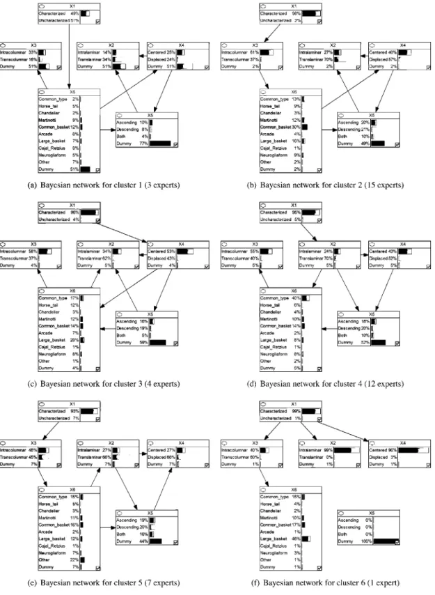
Fig. 7. Network structures and marginal probabilities of the representative Bayesian networks for each cluster. Each one of the Bayesian networks corresponds to a component in the finite mixture of Bayesian networks that builds up the consensus Bayesian multinet.

(13)

•

1 2 3 4 5 6 7 8

Structure learning algorithms

Fig. 8. Comparison between the greedy thick thinning (GTT) algorithm and eight algorithms for learning the Bayesian network structures: (1) HC-K2, (2) TA-K2, (3) MM-K2, (4) RS-K2, (5) HC-BIC, (6) TA-BIC, (7) MM-BIC and (8) RS-BIC. Each boxplot summarizes the 41 Jensen–Shanon divergence values (42 experts minus expert #33) between the JPDs of the Bayesian networks obtained with the GTT algorithm and the JPDs obtained with each one of the eight alternative methods.

explained in Section 3.2.1. The Jensen–Shanon divergence (Eq. (3)) b e t w e e n t h e JPD corresponding t o t h e Bayesian n e t w o r k l e a r n e d w i t h t h e GTT algorithm a n d t h e eight alternative s t r u c t u r e learning m e t h o d s w a s c o m p u t e d . The s t r u c t u r e learning algorithms could n o t b e applied for e x p e r t # 3 3 b e c a u s e h e / s h e classified all t h e n e u r o n s as X2 = Intralaminar a n d t h e algorithms could n o t h a n d l e variables w i t h only o n e value.

Fig. 8 s h o w s boxplots of t h e Jensen–Shanon divergence values (Y axis) b e t w e e n t h e GTT a l g o r i t h m a n d t h e o t h e r e i g h t algorithms (X axis) obtained for t h e 4 1 experts (42 m i n u s e x p e r t # 3 3 ) . Note t h a t t h e JS divergence is b o t h lower a n d u p p e r b o u n d e d : 0 ≤ dJS ≤ 1. W e can see t h a t t h e JS divergence yielded very low values, being almost all of t h e m b e l o w 0.2.

On t h e o n e h a n d , t h e TA-K2 algorithm (second boxplot in Fig. 8) yielded t h e lowest JS divergence values. On t h e o t h e r h a n d , t h e RS algorithm (fourth a n d eighth boxplots in Fig. 8) learned Bayesian n e t w o r k s w h i c h yielded JPDs differing t h e m o s t c o m p a r e d t o t h o s e o b t a i n e d w i t h t h e GTT algorithm. As expected, w e can s e e t h a t algorithms using K2 scoring function yieldedlowerJSdivergences t h a n t h o s e u s i n g BIC,because t h e G T T a l g o r i t h m a l s o u s e d t h e K 2 s c o r i n g f u n c t i o n . W e c o n c l u d e d t h a t t h e algorithm u s e d for learning t h e Bayesian n e t w o r k s t r u c t u r e s did n o t have a n i m p o r t a n t influence in t h e p r o p o s e d methodology because w e u s e d t h e JPDs for clustering t h e Bayesian n e t w o r k s a n d t h e y w e r e similar regardless of t h e applied algorithm.

4.2. Cluster labeling and analysis of the probability distributions

W e identified differences b e t w e e n t h e g r o u p s of e x p e r t s by s t u d y i n g t h e marginal (or prior) probabilities in t h e r e p r e sentative Bayesian n e t w o r k s for each cluster (see Fig. 7) . W e u s e d t h e s e marginal probabilities t o characterize e a c h g r o u p of experts a n d w e i n t e r p r e t e d t h e s e differences a s different a p p r o a c h e s w h e n classifying t h e n e u r o n s :

• Cluster 1 (including t h r e e experts) r e p r e s e n t e d e x p e r t s w h o considered t h a t half of t h e n e u r o n s in t h e e x p e r i m e n t did n o t h a v e e n o u g h r e c o n s t r u c t e d axonal processes for it t o b e feasible t o actually t r y t o classify t h e m . Thus, t h e y assigned t h e n e u r o n s t o t h e Uncharacterized category in X1 (probability 0.51). The probability of Uncharacterized w a s m u c h lower in all t h e o t h e r Bayesian n e t w o r k s ( ≤ 0 . 0 7 ) . In fact, t h e c o m b i n a t i o n of values of t h e variables w i t h higher probability ( m o d e ) c o r r e s p o n d e d t o X1 = Uncharacterized, X2 = Dummy, X3 = Dummy, X4 = Dummy, X5 = Dummy a n d X6 = Dummy.

• Cluster 2 included 15 e x p e r t s w i t h a coarse classification s c h e m e . In this Bayesian n e t w o r k , m o s t of t h e n e u r o n s w e r e classified a s Common basket (0.30). The m o d e of t h e JPD e n c o d e d in t h e representative Bayesian n e t w o r k w a s X1 = Characterized, X2 = Intralaminar, X3 = Intracolumnar, X4 = Centered, X5 = Common basket a n d X6 = Dummy. • Cluster 3 (including four experts) r e p r e s e n t e d e x p e r t s w h o stuck t o t h e fine-grained classification s c h e m e p r o p o s e d

i n t h e e x p e r i m e n t a n d tried t o distinguish b e t w e e n t h e different n e u r o n a l t y p e s , including t h e difficult o n e s such a s Common basket, Common type, Large basket a n d Arcade cells. Experts in this cluster found m o r e Arcade cells (0.07) t h a n t h e e x p e r t s in t h e o t h e r clusters. In this cluster, Common type (0.17), Common basket (0.14) a n d Large basket (0.20) cells h a d similar probabilities. The m o d e of t h e JPD e n c o d e d by t h e representative Bayesian n e t w o r k w a s t h e s a m e a s in cluster 2 .

(14)

Bayesian n e t w o r k wasX1 = Characterized,X2 = Translaminar,X3 = Intracolumnar,X4 = Centered,X5 = Common type and X6 = Dummy.

Cluster 5 represented a group of seven experts with a detailed classification scheme, since they distinguished between

Common type, Common basket and Large basket cells. However, the experts did not seem to agree with the nomen clature included in the experiment or found it incomplete. This was observed in the high probability of the category

Other (0.22) inX6, where they could propose an alternative name for that class of neurons. Interestingly, the mode of theJPD of the representative Bayesian network for this cluster was X1 = Uncharacterized,X2 = Dummy, X3 = Dummy,

X4 = Dummy, X5 = Dummy and X6 = Dummy. In fact, we can see that this cluster assigned the second highest probability to Uncharacterized in all t h e clusters.

Cluster 6 included only one expert with a remarkably different behavior than the other experts. This expert did not classify any neuron as Translaminar inX2, so the probability of that value in the representative Bayesian network is almost 0. Also, this expert assigned a very high probability to Centered inX4 (0.96). Therefore, X5 was disabled for all the neurons (recall thatX5 was only available when Translaminar and Displaced were set as values inX2 andX4, respectively). Therefore, X5 had a constant Dummy value in Fig. 7(f). The conclusions of the analysis of the mode of the JPD were the same, as the combination of values of the variables with highest probability was X1 = Characterized,

X2 = Intralaminar,X3 = Transcolumnar,X4 = Centered,X5 = Large basket andX6 = Dummy.

4.3. Analysis of the Bayesian network structures

Similarities in the behaviors of all the group of experts were identified by analyzing the representative Bayesian network structures. Variables X3 and X6 were the only two variables which were directly related in all the Bayesian networks. Variable X3 describes the neuronal morphology in the horizontal dimension. This feature encodes whether or not the axonal arborization of the neuron extends more than 300 μm from the soma. This means that the interneuron contacts with neurons inside and outside its cortical column, so we could conclude that some neuronal types mainly connect with other neurons from the same cortical column, whereas other neuronal types connect additionally with neurons from different cortical columns.

Additionally, variablesX2,X4 andX5 were related in all but one Bayesian network, the one corresponding to cluster 6. Also, there was an edge between X5 and X6 in all the Bayesian networks but the one for cluster 6. Note that cluster 6 contained only the outlying expert 33. Variables X2, X4 and X5 are mainly related to the neuronal morphology in the vertical dimension. These relationships could determine whether a given neuronal type sends the information to other neurons in the same cortical layer or in different (either upper or lower) layers. We also analyzed the Markov properties of the representative Bayesian network structures to identify conditional independence relationships between the variables.X3 was conditionally independent of variables (X2, X4, X5) given the value of X6 and X1. Therefore, the morphological properties of GABAergic interneurons in the horizontal and vertical dimensions seemed to be independent given the neuronal type.

4.4. Finding agreed definitions for neuronal types using inference in Bayesian networks

The representative Bayesian n e t w o r k s w e r e u s e d t o infer t h e m a i n p r o p e r t i e s of t h e different n e u r o n a l t y p e s in X6 by setting evidence in s o m e variables a n d u p d a t i n g t h e probabilities in t h e u n o b s e r v e d variables. W e s t u d i e d t h e p r o p a g a t e d probabilities a n d identified differences a n d similarities b e t w e e n clusters. Cluster 6 c o r r e s p o n d e d t o a n outlier e x p e r t w h i c h h a s already b e e n analyzed, s o w e focused o n t h e o t h e r five clusters. First, t h e m a i n morphological p r o p e r t i e s of t h e n e u r o n a l t y p e s w e r e found by setting every value in X6 as evidence a n d propagating t h e probabilities using t h e clustering algorithm [6 3,6 4] in GeNIe:

• Martinotti cells w e r e defined as Translaminar (≥0.94), Displaced (≥0.83) a n d Ascending (≥0.57) cells. Experts i n cluster 5 classified t h e s e n e u r o n s a s mostly Transcolumnar (0.73), w h e r e a s t h e y w e r e classified in clusters 1, 2, 3 a n d 4 as either Intracolumnar or Transcolumnar w i t h similar probabilities.

• Horse-tail cells s e e m t o have a c o m m o n a n d easily recognizable morphology, since t h e m o s t likely values achieved high probabilities in all t h e c l u s t e r s : Translaminar (≥0.92), Intracolumnar (≥0.80), Displaced (≥0.88) a n d Descending (≥0.50).

• Chandelier cells s e e m e d t o b e mainly Intracolumnar (≥0.72). However, t h e y w e r e classified a s e i t h e r Intralaminar or Translaminar a n d Centered or Displaced in different clusters. Clusters 2 a n d 4 assigned a higher probability t o Translaminar, cluster 3 assigned a higher probability t o Intralaminar a n d t h e probabilities w e r e almost uniform in t h e X3 variable in clusters 1 a n d 5. Centered received a higher probability in cluster 3 , w h e r e a s t h e probabilities w e r e m o r e uniform in t h e o t h e r clusters.

(15)

• Common type cells w e r e characterized a s Translaminar (≥0.62) cells. Experts in clusters 4 a n d 5 classified t h e m as either Intracolumnar or Transcolumnar, w h e r e a s e x p e r t s in clusters 1, 2 a n d 3 selected Intracolumnar a s t h e m o s t likely value (≥0.66).

• The p r o p e r t i e s for Common basket cells could n o t b e easily identified. Experts in cluster 2 a n d 4 classified m o s t of t h e m as Translaminar (≥0.63), cluster 3 assigned t h e highest probability t o Intralaminar (0.82), w h e r e a s in t h e o t h e r clusters they w e r e classified a s either Translaminar or Intralaminar. Intracolumnar w a s always m o r e likely t h a n Transcolumnar, a l t h o u g h t h e differences in t h e probability values greatly varied in t h e clusters. W e also found major d i s a g r e e m e n t s in X4: Clusters 1 a n d 3 assigned Centered w i t h a high probability (≥0.86), w h e r e a s t h e probabilities of Centered a n d Displaced w e r e similar i n t h e o t h e r clusters.

• Large basket cells w e r e characterized as Translaminar (≥0.58) a n d Transcolumnar (≥0.63) cells. Clusters 1 a n d 3 defined t h e m a s mainly Centered (≥0.74), cluster 5 assigned a higher probability t o Displaced (0.6), w h e r e a s in t h e o t h e r clusters Centered a n d Displaced h a d m o r e uniform probabilities.

• Arcade cells w e r e frequently classified as Translaminar (≥0.65), Intracolumnar (≥0.55) and, w h e n Translaminar a n d Displaced w e r e selected, as Descending cells.

• Most of t h e n e u r o n s classified a s Other w e r e characterized a s Translaminar (≥0.62). Intracolumnar w a s m o r e likely t h a n Transcolumnar i n all t h e clusters. Also, Displaced h a d a higher probability t h a n Centered in all t h e clusters, except for cluster 6. However, t h e differences b e t w e e n t h e probabilities of t h e s e values greatly varied from cluster t o cluster. Cluster 3 yielded a high probability for Both category in X5 (0.50), w h e r e a s cluster 1 assigned a greater probability t o Descending (0.38). The probabilities in X5 w e r e m o r e uniform in t h e other clusters.

Setting evidence in t h e o t h e r variables also highlighted s o m e differences b e t w e e n g r o u p s of e x p e r t s . For example, s e t ting Intralaminar as evidence in X2 yielded Common basket as t h e m o s t likely value for X6 in all t h e Bayesian n e t works, except for t h e o n e corresponding t o cluster 4, w h e r e Common type a n d Neurogliaform got higher probabilities. Setting Translaminar as evidence in X2 yielded very different p r o p a g a t e d probabilities in t h e clusters. W h e n setting Intracolumnar a s evidence in X3, t h e m o s t likely values in X6 w e r e Common basket (clusters 1 a n d 2), Common type (clusters 3 a n d 4) a n d Other (cluster 5).

The c o n s e n s u s Bayesian m u l t i n e t w a s u s e d t o perform inferences taking into account all t h e representative Bayesian n e t w o r k s at t h e s a m e t i m e . The probability of a given q u e r y w a s c o m p u t e d using t h e finite m i x t u r e of Bayesian n e t w o r k s expression (Eq. (6)). Table 1 s h o w s t h e conditional probabilities of each variable given t h e n e u r o n a l t y p e in X6. W e u s e d t h e s e conditional probabilities to infer a set of agreed definitions for s o m e n e u r o n a l t y p e s :

• Martinotti cells w e r e usually classified as Translaminar, Displaced a n d Ascending.

• Horse-tail cells w e r e c o m m o n l y defined a s Translaminar, Intracolumnar, Displaced a n d Descending n e u rons.

• A c o m m o n feature of Chandelier n e u r o n s w a s t h a t t h e y w e r e Intracolumnar.

• Neurogliaform cells w e r e mainly Intralaminar, Intracolumnar a n d Centered cells. • Common type cells w e r e primarily Translaminar.

• Large basket n e u r o n s w e r e characterized a s Translaminar a n d Transcolumnar. • Arcade n e u r o n s w e r e usually classified a s Translaminar.

• N e u r o n s classified as Other w e r e c o m m o n l y classified a s Translaminar a n d Intracolumnar cells.

4.5. Clustering visualization with PCA

The clusters o b t a i n e d w i t h K-means w e r e visually inspected using a r e p r e s e n t a t i o n in a lower d i m e n s i o n a l space. The goal w a s t o obtain a t h r e e - d i m e n s i o n a l r e p r e s e n t a t i o n t h a t a p p r o x i m a t e s t h e 121-dimensional JPDs a n d check w h e t h e r or not t h e clusters w e r e visually distinguishable. A principal c o m p o n e n t analysis (PCA) w a s performed, a n d t h e t h r e e p r i n cipal c o m p o n e n t s w h i c h account for t h e highest p r o p o r t i o n of variance (67.14%) w e r e s t u d i e d [65]. Fig. 9 plots t h e values of t h e JPDs for e a c h e x p e r t in t h e t r a n s f o r m e d t h r e e - d i m e n s i o n a l s p a c e . Different s y m b o l s a n d colors w e r e u s e d t o s h o w t h e cluster assigned by t h e K-means algorithm t o e a c h expert. Two-dimensional projections w e r e also included for e a s e of interpretation. Also, w e s t u d i e d t h e w e i g h t s associated w i t h each JPD value in each o n e of t h e principal c o m p o n e n t s (PCs):

• The first PC, w h i c h a c c o u n t e d for 47.32% of t h e variance, distinguished t h e e x p e r t s in cluster 1 from t h e o t h e r clusters. In this PC, t h e value of t h e JPD w i t h highest (absolute) w e i g h t w a s X1 = Uncharacterized, X2 = Dummy, X3 = Dummy,

X4 = Dummy, X5 = Dummy, X6 = Dummy (weight = 0.9828). The second w e i g h t w i t h t h e largest absolute value h a d a value equal t o -0.06119. This PC primarily s e p a r a t e d e x p e r t s w i t h different behaviors w h e n classifying t h e n e u r o n s as either Characterized or Uncharacterized in variable X1. Therefore, t h e t h r e e experts in cluster 1 (Fig. 7(a)), w h i c h classified a lot of n e u r o n s as Uncharacterized, w e r e easily distinguished using this PC.

(16)

Table 1

Conditional probabilities of each variable given the neuronal type (X6), computed with the consensus Bayesian multinet. The largest value for each conditional probability distribution is highlighted in boldface.

Common type

Conditional probabilities P(X1|X6)

Characterized 0 . 9 9 8 9

Uncharacterized 0.0011

Intralaminar 0.2847 Translaminar 0.7136

Dummy 0.0017

Intracolumnar 0.6190

Transcolumnar 0.3802 Dummy 0 . 0 0 0 8

Centered 0 . 4 2 9 3 Displaced 0 . 5 6 9 6

Dummy 0.0011

Ascending 0.1623 Descending 0.2169 Both 0.1296

Dummy 0.4912

Horse-tail 0.9981 0.0019 0.0720 0.9254 0.0026 0.8639 0.1346 0.0015 0.1088 0.8893 0.0019 0.1244 0.6439 0.1119 0.1198 Chandelier 0.9962 0.0038 0.4270 0.5671 0.0059 0.7903 0.2065 0.0032 0.5292 0.4668 0.0040 0.0950 0.1961 0.0754 0.6335 Martinotti 0.9988 0.0012 0.0632 0.9350 0.0018 0.4001 0.5990 0.0009 0.1151 0.8837 0.0012 0.6479 0.1103 0.1187 0.1231 Common basket 0.9992 0.0008 0.4477 0.5511 0.0012 0.6862 0.3132 0.0006 0.6075 0.3917 0.0008 0.1008 0.1270 0.0790 0.6932 Arcade 0.9937 0.0063 0.2863 0.7057 0.0080 0.6365 0.3579 0.0056 0.4078 0.5856 0.0066 0.1290 0.2606 0.1311 0.4793 Large basket 0.9988 0.0012 0.2642 0.7342 0.0016 0.1874 0.8117 0.0009 0.5126 0.4862 0.0012 0.1630 0.1762 0.1096 0.5512 Cajal-Retzius 0.9835 0.0165 0.2947 0.6817 0.0236 0.4687 0.5165 0.0148 0.3833 0.5997 0.0170 0.1852 0.2259 0.1553 0.4336 Neurogliaform 0.9983 0.0017 0.6806 0.3170 0.0024 0.8589 0.1398 0.0013 0.7524 0.2459 0.0017 0.0400 0.0369 0.0302 0.8929 Other 0.9950 0.0050 0.2423 0.7491 0.0086 0.7242 0.2716 0.0042 0.3410 0.6540 0.0050 0.1859 0.2106 0.2252

0 3 7 8 3

Dummy 0.0115 0.9885 0.0072 0.0081 0.9847 0.0030 0.0030 0.9940 0.0052 0.0055 0.9893 0.0036 0.0036 0.0036 0.9892

X3 = Transcolumnar, X4 = Centered, X5 = Large basket, X6 = Dummy (weight = -0.7385). Fig. 7(f) s h o w s t h a t t h e representative Bayesian n e t w o r k of t h e outlying e x p e r t in cluster 6 h a d a very high probability (0.46) for Large Basket cells. Therefore, this PC s e p a r a t e d t h e e x p e r t in cluster 6 from t h e rest of t h e clusters.

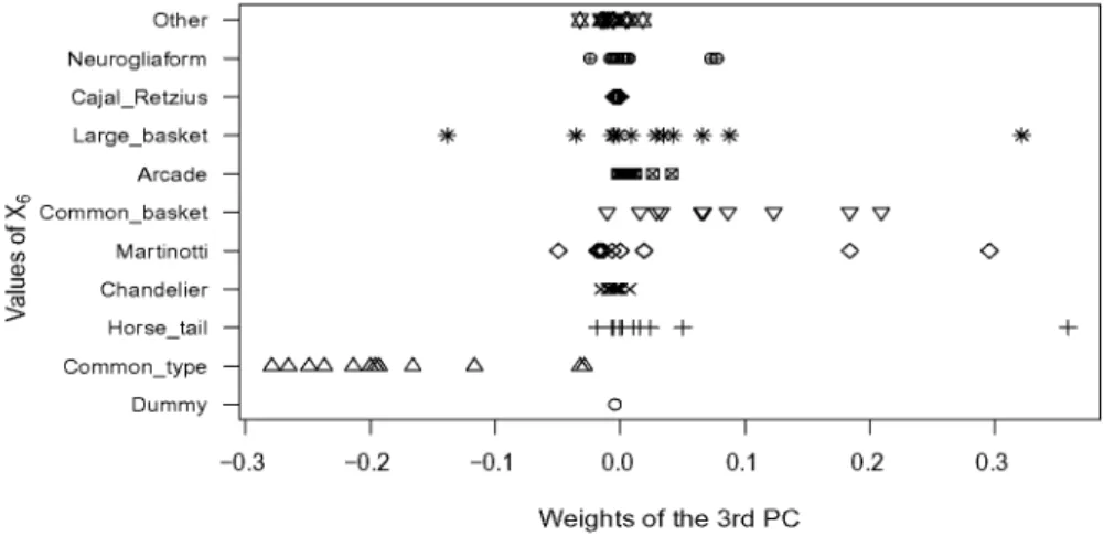
• The third PC accounted for 9.08% of t h e variance a n d could n o t easily s e p a r a t e t h e rest of t h e clusters. However, this PC s e e m e d t o b e able t o distinguish b e t w e e n e x p e r t s in cluster 2 a n d e x p e r t s in cluster 4. These t w o clusters c o n t a i n e d e x p e r t s w i t h t w o different behaviors. Fig. 7(d) s h o w s t h a t t h e e x p e r t s in cluster 4 classified m o s t of t h e n e u r o n s as Common type (0.40), w h e r e a s t h e e x p e r t s in cluster 2 (Fig. 7(b)) classified m o s t of t h e n e u r o n s a s Common basket (0.30). Clusters 3 a n d 5 w e r e less distinguishable b e c a u s e t h e probability w a s m o r e uniformly distributed across t h e values in X6 (Fig. 7(c) a n d (e)). The w e i g h t s in t h e third PC w e r e also h a r d e r t o interpret. However, cluster 4 a n d cluster 2 could b e distinguished. All t h e values of t h e JPD w i t h X6 = Common type h a d w e i g h t s smaller or equal t h a n - 0 . 0 2 8 5 9 , w h e r e a s all t h e values w i t h X6 = Common basket h a d w e i g h t s greater or equal t h a n - 0 . 0 1 0 2 (see Fig. 10). Therefore, t h e set of values w i t h X6 = Common type (cluster 4) a n d X6 = Common basket (cluster 2) w e r e disjoint according t o t h e third PC.

W e concluded t h a t t h e behavior of e x p e r t s in clusters 1 a n d 6 w a s remarkably different from t h e behavior of t h e rest of t h e e x p e r t s . The K-means algorithm w a s able t o identify t h o s e characterizing behaviors a n d g e n e r a t e d t w o different clusters for t h e m . Additionally, differences b e t w e e n t h e e x p e r t s in clusters 2 a n d 4 w e r e also correctly identified. The differences b e t w e e n clusters 3 a n d 5 w e r e m o r e subtle a n d it w a s difficult t o find a t h r e e - d i m e n s i o n a l r e p r e s e n t a t i o n of t h e JPDs w h i c h s e p a r a t e d t h e s e experts.

4.6. Geographical identification of the clusters

(17)

0.2

0.1

-0.1

-0.2 _-0.4

-0.2 2nd PC

-0.2 0.2 0.6

1st PC

0.0 0.2 0.4

1st PC

0.6

Ho D o»GS

SsSr

°<?x

0

V

0

X

O V

Cluster 1 Cluster 2 Cluster 3 Cluster 4 Cluster 5 Cluster 6

0.0 0.2 0.4

1st PC

0.6

Fig. 9. Visualization of the clusters computed with K-means (K = 6) in three and two-dimensional spaces obtained with principal component analysis. The three-dimensional coordinates of the experts correspond to the values of the three principal components with highest proportion of variance.

Other

Neurogliaform

Cajal_Retzius

Large_basket

Arcade

Common_basket

Martinotti

Chandelier

Horse_tail

Common_type

Dummy

^ 3B9K 3HSK 3£ ^K

V W V V V V V

o «es>o o o

AAAA A m A A

-0.3 -0.2 -0.1 0.0 0.1 0.2 0.3

Weights of the 3 r d P C

Fig. 10. Weights of the third principal component according to the value of the variable X6 in the JPD.

5. Conclusions

Bayesian networks have been successfully applied to a wide range of problems in very different domains. In this paper, we have presented a methodology for building a consensus Bayesian multinet that represents the opinions of a set of experts. The methodology canbesummarizedinthreesteps. First,aBayesian networkislearned for each expert. Second, the Bayesian networks corresponding to experts with similar behaviors are clustered. Third, a consensus Bayesian multinet is built which