A model f o r t h e s i m u l a t i o n o f energy gains w h e n using
distributed m a x i m u m p o w e r point t r a c k i n g ( D M P P T ) in
photovoltaic arrays
Jorge Solórzano-Moral , Daniel Masa-Bote, Miguel Angel. Egido-Aguilera
and Estefanía Caamaño-Martín
ABSTRACT
Over the past years, the photovoltaic (PV) market has been invaded with numerous power optimizers and micro-inverters that claim large energy gains when used in PV generators with shading or module mismatch. These products provide distributed maximum power point tracking (DMPPT), normally at module level, allowing the maximum power to be extracted from each PV module. This topology can be beneficial in situations where the PV generator is shaded or when there is large module mismatch. However, it is not clear that this power gain will result in energy improvements over a whole year or the lifetime of the system. This paper presents a very detailed and precise model for simulating energy gains with DMPPT as well as its verification and simulation results with different shading profiles, showing the possible energy gain over a whole year. Simulation results show that the yearly energy gain is much lower than the maximum power gain. However, interesting yearly gains of up to 12% are obtained in one of the simulations. Copyright © 2013 John Wiley & Sons, Ltd.
KEYWORDS
distributed MPPT (DMPPT); power optimizers; micro-inverters; mismatch; energy optimization; shadows
1. INTRODUCTION
Photovoltaic (PV) systems in the urban environment are known to be more affected by shadows and dirt than ground-mounted systems. This will cause losses because of less incident radiation and will also cause losses because of mismatch between modules in centralized maximum power point tracking (MPPT). The use of distributed MPPT (DMPPT) at module level, whether power optimizers or micro-inverters, allows the independent MPPT of each module, solving part of the problems related to partial shadows, localized dirt, or mismatching, and makes it possible to connect PV modules with different characteristics and tilt or orientation angles.
Although the idea of using micro-inverters has been present since the early 1990s [1] [2] and that of power optimizers since the mid-2000s [3], it has not been until the last couple of years that these products have invaded the market, and by the end of 2011, there were over 15 companies offering power optimizers and at least five
offering micro-inverters [4]. The common denominator in the claims made by these companies is the extra electricity produced by the use of their products, some claiming "extra power yields up to 30%" and others even claiming "up to 25% extra energy harvests".
In previous work [5-7], various experimental tests have been undertaken that verify power improvements due to different shading profiles. Various power improvement factors, normally not only around 10-15% but also up to 34%, can be observed as a function of the shade applied, the proportion of affected and non-affected modules, and also the interconnection of the modules; series-connected strings are more vulnerable than parallel-connected ones.
which is similar to the ones observed in previous work, only a 1% annual energy gain will be obtained.
These improvement factors depend on the effect that shading of PV cells has on each module's IVcurve, which at the same time depend on their reverse characteristics. In other work [9,10], simulation models and experimental studies of the effects of shading on the I-V curve of a module have been conducted, and these, combined with the analytical models and field results previously presented [5], have served as the base for a simulation model of the behavior of PV generators with DMPPT converters.
The objective of this paper is to present a very detailed and precise simulation model for the estimation of possible energy improvements with the use of DMPPT techniques, as well as its verification, and simulation results of different PV generators with different shading patterns and module characteristics. No differentiation is made between power optimizers and micro-inverters because their only difference is that power optimizers are connected in DC and micro-inverters in alternating current (AC). Theoretically, they could both reach the same energy improvement.
2. DESCRIPTION OF THE MODEL
The different tests that have been performed on DMPPT techniques in [5-7] have all been performed with real products and under real conditions. In [5] and [7], the devices were tested under real sun conditions, and the whole generator, while under the same shade and practically at the same irradiance and temperature, was quickly switched from DMPPT to MPPT, and the power improvement was recorded. In [6], thanks to the use of a large sun simulator, the tests were conducted in the laboratory, and two generators were used, one with power optimizers and one without. However, these techniques are only suitable for measuring power improvements and not for energy improvements over an extended period of time with varying irradiation and sun position.
In order to perform energy improvement tests under real conditions, two exact generators (two sets of identical I-V curves) under the exact same shading pattern and exposed to the same irradiance and temperature have to be under test for at least 1 year to consider all of the sun's positions and different irradiance and temperature conditions. Even if the exposed requirements are met, needing 1 year for each shading pattern makes this process not practical. In addition, these tests will be limited to weather patterns of only one location.
Considering these difficulties, it seems reasonable that a suitable model for simulating energy gains with DMPPT should be developed. For a detailed and precise analysis, this model should consider, at least, the following points:
• The sun's relative position for a whole year with respect to the location (mainly latitude) of the generator. • Direct and diffuse components of the solar radiation
during every time period.
• The shading profile on each module down to the cell level.
• The distinct I-V curve of each module of the generator.
• The reverse characteristics of the I-V curve: these, when a cell is shaded, influence the I-V curve of the whole module and, therefore, that of the whole generator.
2 . 1 . Solar radiation model
The radiation data for Madrid used for this model come from a weather station installed on the roof of the Instituto de Energía Solar building at Madrid, Spain, exactly at 40.5°N and 3.7°W. For this model, 1-min interval values of direct horizontal radiation, B(0), diffuse horizontal radiation, D(0), and air temperature, Ta¡ are used. These
values are averaged according to the time interval of the simulation.
The radiation data used for the Stuttgart location were obtained from Meteonorm. Hourly values of B(0), D(0). and Ta were obtained from the program.
These data are then converted to the tilt and orientation angles of the generator [11], with basic trigonometry for the beam radiation through equation [1].
B(a,fi)
B(0)-max(0, cos(9scos 67, (1)
Where cos6s is the incidence angle of the sun's rays
over the surface, and cos6zs is the zenith angle.
The calculation of the diffuse component over the PV generator's surface is calculated using the Perez model [12]. The governing expression in Perez's model is given in equation [2]. The terms in brackets represent radiation, in the following order: from the background, from the circumsolar region, and from the horizon. k3 and k4
repre-sent the contributions of the circumsolar and horizon regions to diffuse irradiation, a and c are, respectively, the values of the solid angle of the circumsolar region as seen from a surface with slope/? and from a horizontal surface.
Dt(a,p) = A(0) ' 1 - f a
(1 + cos/?) a
ki - + ki, sin/?
c
(2)
With the exception of snowy grounds or vertically placed modules, the contribution of the reflected components is usually very small. For this model, the reflected component has not been considered.
The global radiation over the PV generator's surface is obtained with the sum of the two components as in [3]:
Shades due to obstacles affect each of these components differently. This is explained in the following section.
2.2. Shading profile model
The shading profile module aims to characterize the shadows that affect each individual cell of the PV generator.
First of all, the obstacles surrounding the PV generator must be characterized. The obstacle profile, defined in equation [4], can be obtained from this collection of points.
OP{y,y) =
1; ((//, 7)3 obstacle
0; otherwise ;\¡i= [-180,180],/= [0,90) (4)
The obstacle profile is a two-dimensional function, which describes the location of obstacles in the sky dome; a point in the sky dome is assigned the value of 1 if an obstacle is present or a value of 0 if the point is free of obstacles. The obstacle profile contains all the information necessary to evaluate shadows and, therefore, estimate effective irradiation for the location at which it has been defined.
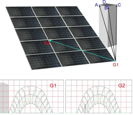
In Figure 1, a representation of how the shadow profile is calculated for a whole PV generator, and the shadow profiles obtained for two different points of the generator, Gl and G2, are shown. The generator is the same as the one that is simulated in Section 4.
First, the location of the top points of the obstacle with respect to the south-eastern most corner of the generator is measured. The obstacle is always considered to be touching the ground, so the bottom points are not necessary.
Because an obstacle profile is only valid for one point in the generator, it is necessary to obtain obstacle profiles for various points on the PV generator's surface. As explained in Section 3.1, we define a rectangular grid over the generator's surface, and a shadow profile for each point in the grid is calculated by translating the points in Table I In this case, in Figure 1, the chimney never affects Gl, whereas it does affect G2 during certain time periods of the year. It can also be seen how the relative size of the obstacle decreases very quickly in a short distance. This indicates the importance of simulating the shadow profile down to the cell level, because in just a few cells, the amount of shade can vary in a large amount.
Once the obstacle profile is calculated for every point of the PV generator, it is possible to calculate the radiation that reaches each point.
We consider that points on the generator that are blocked by the obstacle do not receive any direct radiation (beam + circumsolar). This is directly given by the obstacle profile calculated at each point of the PV generator.
For the diffuse radiation, its associated loss factor is the fraction of the sky dome "seen" by the generator, which is blocked by the obstacle. For example, a PV facade with an infinitely high and long wall on one of its sides loses 50% of the diffuse radiation that it "sees" (note that being a facade, it already loses 50% of the sky dome).
s ' A
\ V
.
\ \ ~~?
1 / /
\
-r
t:
V
\
'A J 1Table I. The values obtained from the characterization of the obstacle in Figure 1.
A(x,y,z) B(x,y,z) C(x,y,z) D(x,y,z)
- 0 . 1 , - 0 . 8 2 , 2.76 - 0 . 1 , - 0 . 3 2 , 2.76 - 0 . 6 , - 0 . 3 2 , 2.76 - 0 . 6 , - 0 . 8 2 , 2.76
2.3. I-V curve modeling
It is well known that shadows over PV modules affect their
I-V curves and that this effect is conditioned by the reverse
characteristics of the shaded solar cells [10,13,14]. Despite this, most simulation software does not take the analysis of shadows to the level of the solar cell [15], as opposed to this model.
With the aim of having the most realistic simulation, real I-V curves of different modules have been used, and their reverse characteristics have been simulated. First of all, the I-V curves of 15 modules were measured and extrapolated to standard test conditions. From these curves, and assuming that all cells in the module have the same
I-V curve , the I-V curve of each cell and their equivalent
shunt resistance, Rsh, are calculated. The capacitive load
used for the measurements permits negatively pre-charging it, which ensures the characterization of the curve in a few negative values and in lsc, permitting a more precise
calculation of Rsh.
Rsk is calculated as the slope of the curve from
-Q.2*N*Voc to 0.2*N*VOc, where Ns is the number of
cells in series of the module. The curve of each cell is simply calculated by dividing each of the current values of the module's I-V curve by Ns and the voltage values by the
number of parallel cells, Np, considering all cells equal.
With this done, the next step is calculating the reverse characteristics of the solar cells, also considered equal for all cells. This simplification could also be considered a limitation, especially if there is such a high variability in the reverse characteristics as shown in [9]. However, we will see in Section 4.2 that this is not the case for the measured modules.
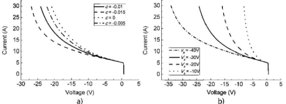
In [16], different models for representing the behavior of PV cells in reverse bias are reviewed, and a new model is proposed and validated, which, in turn, is used in this paper with a slight modification, the introduction of a linear term, b. The model used responds to equation [5]:
1 =
1-lsc-b-Gp-V + c-V2
-exp{
S e(l-^p)}
(5)
Where Be is a non-dimensional quasi-constant parameter
with value a 3, V& is the breakdown voltage, 0r is the built-in junction voltage (not to be used as an adjustable parameter, using a typical value of 0.85 for silicon cells of unknown junction structure.), and Gsh is the shunt conductance,
simply 1/Rsh. The addition of the parabolic term c (c < 0) is
used in cases where the linear fitting is not sufficient, and the linear term b is added to compensate for differences in
Gsk in the second quadrant.
Now, the problem is adjusting the unknown parameters,
Vb, Be, and c, without measuring the module's I-V curve in
the second quadrant. However, it is possible to obtain this by partially shading cells from a module, because the shape of the I-V curve from Pm to where the diode goes into
forward bias (highlighted area of Figure 2) is equivalent to the shape of the I-V curves in reverse bias of the shaded cells. Doing this, we can observe the reverse characteristics of the shaded cell in the first quadrant.
Having information about the reverse characteristics of the solar cells, it is now possible to adjust the unknown parameters of equation [6]. As Be is a quasi-constant
parameter, its adjustable range is very small, that is from 2.5 to 3.5, so the main adjustable parameters will be c and Vb- The effect of varying these two parameters can be seen in Figure 3.
Ideally, these parameters would be adjusted for each cell of all the modules used in the simulations. However, for this work, the parameters represent the average values of the cells in each module, and in Section 3.2, it is shown that this works well enough.
Once the reverse characteristics are modeled, it is now possible to simulate a shaded module, obtaining the shaded
I-V curves. This is performed for every time period of the
simulations, and the process is as follows:
(1) Extrapolate to the conditions of each time period [17].
(2) Calculate the I-V curve of one cell and assume that all the cells in the module have the same I-V curve.
<
r 4
Ü
10 15 20 25 Voltage (V)
30 35
This isa limitation of the model. However, as we will see further on, the effect is not very important.
Figure 2. Region of the I-V curve affected by the reverse
-30 -25 -20 -15 -10 -5 Voltage (V)
a)
30
25
< 2 0
| 15
o 10
5 0
\
\
vt=-40V | / = -30V l/ = -20V - - - l/ = -10V
, \
\ l
\ V
\
v^ ' ^ ^ s
-35 -30 -25 -20 -15 -10 Voltage (V)
b)
Figure 3. Left: effect of varying c; right: effect of varying Vb in the reverse characteristics of a solar eel
(3)
(4)
(5) (6)
(7) (8)
(9)
Simply divide the current by the number of cells in parallel and the voltage by the number of cells in series.
Calculate the cell's I-V curve in the second quadrant.
Use equation [6] with the adjusted parameters. For each cell, multiply the current of each point of the I-V curve by its shading factor.
Add all the cells together to form the module. For the cells in series: add the voltage of each cell for a given current.
For the cells in parallel: add the current of each cell for a given voltage.
2.4. Shading losses and energy gain estimation
Combining the three models described previously, an I-V curve for each module and for each time period in the simulations is obtained.
First of all, the extrapolated I-V curves and the shaded
I-V curves are used to simulate the extrapolated generator
and the shaded generator by simply adding together the
I-V curves in the same way as the cell's I-V curves were
added.
The comparison of the maximum power point (MPP) of the shaded generator's I-V curve and the MPP of the extrapolated generator's I-V curve results in the shading losses.
The energy gain by the use of DMPPT techniques is obtained by adding the MPP of each module's shaded
I-V curves. The ratio between this sum and the MPP of
the shaded generator is the energy gain with the use of DMPPT. It must be noted that this energy gain also takes into account any mismatch in the original I-V curves, so even if there is no shading present, some energy gain could be obtained.
3. VALIDATION OF THE MODEL
All the experimental tests were performed at the roof of the Instituto de Energía Solar in Madrid in days close to the winter solstice and between 10:00 and 14:00 solar time. The equipment used was a PV module, a photographic camera, a computer, an oscilloscope, and an I-V curve tracer.
The PV module used consists of 60 cells in series, in six columns, and three by-pass diodes. Every two columns are protected by one by-pass diode. Pictures are shown in Figure 4.
3 . 1 . Shading profile model
The procedure used for validating the shading profile model consists in projecting shadows over a module from different obstacles, taking a photograph of the shade at a certain time of the day and comparing this photograph with the shading profile obtained from the model.
All the shadows applied to the PV modules were cast by nearby rectangular objects. The exact dimensions and the distance to the modules of the obstacles were measured, and a shading profile for each minute of the day was obtained. For all the shadows measured, the simulated shading profile was in very good agreement with the real shadow cast by the object.
Two differences were observed between the simulation and the real shadow. These were a small displacement in time and an error due to the discrete nature of the simulated shading profile.
The small displacement in time has no worse effect than not matching the irradiance and temperature of the exact moment with the exact shading profile. Being the differ-ence less than 5min, this effect can be considered negligible.
Because of the finite number of points defined in the shading profile, an error, analogous to the quantification error of any digital machine, is inevitable. For the simulations presented in this paper, different resolutions have been used. In this section, shading profiles with a 4 x 4 resolution2 per cell are presented, and the borders of the shadow are
This section presents a series of tests that have been conducted in order to validate the model and to show its precision.
2ln total, for a module of 6 x 10 cells and a 4 x 4 resolution cell, 960 points are modeled.
Figure 4. Shows two pictures of shaded modules, their shadow profile obtained, and the shading percentage of each cell when border
smoothing is applied.
smoothed, as explained in Section 3.2, in order to minimize the error. Therefore, in these simulations, the maximum error is ±12.5% of shade in each cell.
This, at first glance, can seem like an enormous error to consider the simulations as valid. However, we must understand that this is an instantaneous error, and it is far from the overall error; various simulations back it up. There are mainly two reasons for this.
The first one is that the error in a cell is mainly only transferred to an error in the I-V curve when it occurs in the most shaded cell in a diode zone, because it is this cell that limits the current through the series. Once a cell is shaded 100% in one diode zone, the error committed in the shading of the other cells has no influence on the I-V curve.
And second, because the shadows cast by static objects sweep the whole generator from left to right, there will be times when the error is positive and others when it is negative, compensating itself and reducing the final error.
Figure 4 shows two pictures of two shaded modules, their shadow profile (in red) and the percentage of shaded cell estimated with border smoothing. Looking at the picture on the right, we can see that we are underestimating the maximum shade on the fifth column and overestimating the maximum shade on the fourth column. On the picture of the left, there is an underestimation of the maximum shaded cell on the third column. The effects of this are presented in the following section.
3.2. I-V curve modeling
In order to validate the model for simulating shaded I-V curves, various PV modules under different shading profiles have been measured with a capacitive charge. To avoid errors from the extrapolation of the I-V curve to the specific meteorological conditions, a non-shaded I-V curve of the same module was measured instantly prior
to the shaded I-V curve, and it was used to simulate the shaded curves with the same method used in the simulations but avoiding the extrapolation.
First, the parameters Vt, b, and c were adjusted to match as close as possible shading over different cells. For this, various cells of the same module were shaded and the parameters adjusted until a closest match was obtained, showing two examples in Figure 5. The obtained parameters are
• V6 = - 2 7 V
• c =-0.0055
• b = 0.009
These experiments show that curves when only one cell under the same by-pass diode is shaded are the most difficult to adjust. When only one cell on a module is shaded, for the by-pass diode to go into forward bias, the cell must be working at a very negative voltage, and here, a slight difference of these parameters means a large difference on the curve's shape. However, when many cells are shaded, the negative voltage at which each of them works is much lower, and a small difference of these parameters is also a small difference on the curve's shape, see Figure 3.
In conclusion, the precision of simulating increases as the number of shaded cells increases. Therefore, the procedure should be to try and match as well as possible the simulated and real curves of modules with only one shaded cell per by-pass diode knowing that if this is performed well, any type of shade can be simulated with very little error.
7
6
5
4
3
2
0 (
5 10
\
15 20 25
Voltage (V)
a)
Measured — Simulated
\ \
\ \ \
\
i
\
30 35
<
I
40 6
5
4
3
2
0
(
~ „
5 10
\
15 20 25
Voltage (V)
b)
30 Measured Simulated
\
i 35 4
Figure 5. Shows the measured and simulated l-Vcurves with shading on different cells. The two graphs are shade over 50% of one
cell; 12% over another on different by-pass diodes; and 50%, 25%, and 12% over three different by-pass diodes.
Measured 4x4 • • 8x8
15 20 25 30 35
Voltage (V)
a)
5
4
<
~ 3 c <D
§ 2 O
1
" '-' -V: ,
V
- -
4x4 Measured •8x8V
\
1
\
15 20 25 30 35 40 Voltage (V)
b)
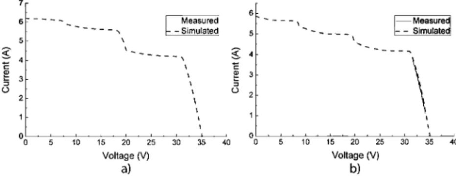
Figure 6. Shows the measured and simulated l-Vcurves of profile from Figure 4 for different resolutions.
Each figure compares the measured I-V curve with two simulated curves: one with a 4 x 4 resolution in each cell and one with an 8 x 8 resolution in each cell, affecting the resulting curve.
It must be understood that the shade presented of the solid object of Figure 4 is very rare. The tiny bit of shade on the third column and second by-pass diode area is what makes it very difficult to simulate correctly. On the other hand, the thin object will always cast shadows, which are difficult to simulate without a high resolution. More on this will be presented in Section 5.
Finally, the validation of a shaded generator is performed. For this purpose, six un-shaded PV modules were measured independently. Afterwards, they were connected together,
different shading profiles were applied to the full generator, and the I-V curves of the shaded generator were measured. In this case, an extrapolation was performed in irradiance; however, the difference between maximum and minimum irradiance during all the measurements was only 1.3%. The cell temperature was assumed constant.
Figure 7 shows the measured and simulated I-V curves of a whole generator when partial shading is present. The graph on the left represents an 85% shade on five cells of one module and one by-pass diode and 27% on two cells of another module also in only one by-pass diode. The graph on the right corresponds to four fully shaded cells in one module and two by-pass diodes, another two cells shaded only 60% in the third by-pass diode and the shadow
Measured - Simulated
50 100 150
Voltage (V)
a)
Measured - Simulated
~\
50 100 150 200
Voltage (V)
b)
cast by a large pole in two by-pass diode zones of another module, at different percentages.
In this case, module mismatch is also present and is taken into consideration. From the comparison of both curves, it can be observed that the simulation of shaded generators also complies very well with reality.
4. PERFORMED SIMULATIONS
Now that the model is validated, it can be used to simulate the energy gain obtained with the use of DMPPT in different situations. All of the following simulations are yearly, considering the sun's relative position and the different irradiance and ambient temperature at every time period.
It is important to note that all the energy gains presented do not take into account the efficiency of the DMPPT equipment. This is due to the large amount of products with different efficiencies and the difficulty to consider them all. In addition, some power optimizers already offer a 98.5% European efficiency [18] and considering that their inverter could have a higher efficiency than normal inverters, because it works at a constant optimum voltage, it is possible that DMPPT can have efficiencies as high as central MPPT techniques. This must be taken into account and know that the results presented here are the maximum possible, being the real ones possibly lower or higher depending on the efficiency of the power optimizers and micro-inverters.
In this model, it has been assumed that the efficiency of the MPPT of both the central inverter and the distributed techniques are equal.
All the simulations presented only consider irradiance values over 200 W/m2.
In these simulations, no module mismatch was considered. Measurements of 15 new modules were conducted, and less than a one-percentage power loss was observed when connecting them in series with respect to adding their power independently. However, the situation were a larger module mismatch is present would be even more beneficial in the case of DMPPT.
When considering energy gains, two different concepts are usually taken into consideration: one is the percentage of recovered energy, ER. That is, of all the energy lost,
how much is recovered. And the other is the improvement in energy, E¡, with respect to the centralized MPPT system; how much better is the DMPPT system than the MPPT system. They are both presented in equations [6] and [7].
„ EDMMPT — EMPPT , , ,
Ei = (6)
c-MPPT
„ EDMMPj — EMppj
Where EDMPPT represents the generated energy with
DMPPT, EMPPT represents the energy generated with a centralized MPPT, and £M A X represents the maximum
possible extracted energy, that is the sum of the energy generated by each individual module considering there are no shadows.
It can be observed that ER has a maximum value of
100%, in the case that all the energy is recovered and
EDMPPT=EMAX- This would happen, for example, in the
case of mismatch between modules when no shading is present.
On the other hand, E¡ does not have a maximum limit; it can have values over 100%, although it is not normally the case.
The recovered energy tends to have a much higher value, and commercial firms tend to use both values, sometimes focusing more on ERt probably for marketing purposes.
However, it must be understood that the real important value is E¡, and if this value is low, there will be no interest in using DMPPT even if ER is 100%.
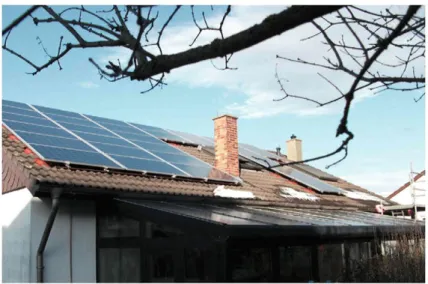
4 . 1 . Single-family household
The first system that has been simulated is shown in Figure 8. It corresponds to a 34° tilted and south facing house roof with a chimney, which shades part of the modules. The house is located in Stuttgart, Germany, and it already incorporates power optimizers.
The generator is composed of two series-connected strings of 15 modules, each connected to a 3.3-kW inverter. For the simulation, only one string has been simulated, which corresponds to the series connection of the five bottom rows of the modules to the left of the chimney; the other one is practically free of shadows.
The chimney has been modeled as a rectangular cube with a 50 x 50cm base and a 2-meter height on its shorter side. It is separated 10 cm from the string, and its top left corner coin-cides with the top right corner of the bottom row of modules.
Various annual simulations with different parameters have been performed; the resolution of the shadow profile has been varied, radiation data from Madrid and Stuttgart has been used, and different shading profiles (and shading losses) for each location have been calculated; taking into account the relative position of the sun in both regions.
Table II shows the results obtained in each simulation for different resolutions with a 15-minute time step.
In addition, the same simulations were performed, but the obstacle was changed to model an antenna. Everything was kept the same except for the size of the base, which was changed to 5 x5cm. The results obtained are shown in Table III. In this case, an even higher resolution, of 16 x 16, was used, having Matlab (The Math Works Inc., Massachusetts, USA) running for over 48 h.
From the previous two tables, we can observe the importance of considering the amount of shade on individual cells for simulating energy gains with DMPPT. When simulating large objects, a 2 x 2 resolution is probably more than enough. However, in objects like antennas, at least a 4 x 4 resolution should be used.
Figure 8. Image of the photovoltaic system used for the simulations.
Table II. Annual simulation results with different parameters for the system of Figure 8.
Resolution Maximum possible energy Energy lost without DMPPT Maximum gain
1 x1 2x2 4x4
6.7 MWh 6.7 MWh 6.7 MWh 6.7 MWh
673 kWh (10.1%) 643 kWh (9.6%) 662 kWh (9.9%) 667 kWh (10%)
26.3% 27.4% 28.2% 28.7%
38.4% 31.8% 32.3% 32.1%
4.29% 3.38% 3.55% 3.55%
DMPPT, distributed maximum power point tracking
Table III. Simulation results changing the chimney for an antenna.
Resolution Maximum possible energy Energy lost without DMPPT Maximum gain
1 x1 2x2 4x4 8x8 16x16
6.7 MWh 6.7 MWh 6.7 MWh 6.7 MWh 6.7 MWh
281 kWh (4.2%) 362 kWh (5.4%) 431 kWh (6.4%) 449 kWh (6.7%) 452 kWh (6,8%)
14.8% 22.5% 31.5% 29.5% 30%
77.7% 78.6% 73.3% 67.1% 65.9%
3.4% 4.49% 5.04% 4.82% 4.76%
DMPPT, distributed maximum power point tracking
less than 1%. However, the difference in energy gain is around 20%. This brings to our attention that although a model that does not consider the amount of shade on individual cells, like in [19], can be accurate in determining shading losses, it is not enough for estimating energy gains with DMPPT.
We can also see that although the antenna is responsible for less energy losses, because of the high energy recovered,
ER, the final energy improvement, E¡, is higher and,
therefore, also the interest in using DMPPT. This coincides with the results obtained in [7] and [5], which show that higher energy gains are obtained for shadows that do not cover entire cells.
The large difference between the maximum instantaneous gain and the total yearly gain should also be observed. This corroborates the hypothesis formulated in [5] and [8], which
stated that although large instantaneous power gains are possible, the overall yearly gain would be much lower, because of various factors like the stationary nature of the objects (shade during only one part of the day) and the different position of the sun throughout the year (higher means less shade). Both maximum gains occur close to the winter solstice, 21st of October and 13th of December for the chimney and antenna, respectively, and in the first period of the day as is expected because of the lower elevation of the sun and longer shadows. However, because of the low energy of that period, it does not contribute in a large manner to the total annual gain.
Table IV. Simulation results for radiation data of Stuttgart, Germany.
Obstacle Shadow profile Maximum possible Energy Energy lost without DMPPT Maximum gain
Antenna Antenna Chimney Chimney
Stuttgart Madrid Stuttgart
Madrid
4.71 MWh 4.71 MWh 4.71 MWh 4.71 MWh
184kWh(3.91%) 250 kWh (5.31 %) 361 kWh (7.67%) 450 kWh (9.54%)
25.4% 30% 22% 20.7%
74.7% 71.5% 40.4% 37.1 %
3.04% 4.01 % 3.36% 3.91 %
DMPPT, distributed maximum power point tracking
(4x4 resolution) with radiation data and a shadow profile from Stuttgart (higher percentage of diffuse radiation and different sun position throughout the year). The yearly radiation data used for Madrid summed up to 1720kWh with a 29% of diffuse radiation on a horizontal plane, whereas that of Stuttgart summed up to 1250 kWh with a 45% of diffuse radiation. The results are shown in Table IV.
From this last simulation, we can observe that in the case of large objects close to the PV generator, such as the chimney, the diffuse fraction is also important, obtaining a little more energy gain when the percentage of diffuse radiation has increased (compare the last result of Table IV with the 4 x 4 resolution result of Table II). This is due to the fact that the modules close to the chimney are losing a large part of their diffuse radiation during all hours, which creates a constant mismatch in the PV generator and, therefore, a constant energy gain.
This is, however, not true for thin objects, like the antenna. For the case of the antenna, 66% less energy gain is obtained in Stuttgart as compared with Madrid.
4.2. Building in an urban environment
Figure 9. Front viewof the urban photovoltaic systemsimulated.
Voc-ln
v(i)=-
ta(2) Rs-hc-RsV-h
Voc(8)
In addition to the previous system, a PV installation in a more complex and in a more urban environment has been simulated. It is a 5-kW PV system right in the center of Madrid, Spain, belonging to the Institute for Research in Technology (IIT-ICAI). The installation faces 18° west, and the modules are tilted on a 29° angle. The 40 modules are grouped into five parallel connected strings of eight modules in series each. The modules are numbered from left to right and from bottom to top. Being the right-most module of the second row from the bottom, module number 13. The five strings are modules 1-8, 9-16, 17-24, 25-32, and 33-40, respectively. Other pictures of the installation can be seen in Figure 9.
The modules of the installation are the ATERSA A120 model, of the following characteristics: PM=120W. V, :16.9 V, yo c= 2 1 V , /M=7.1A, a n d /s c = 7.7A
Because it was not possible to stop the system from working and measure all the module's I-V curves, the exponential model of equation [9] was used to simulate the I-V curve of one module. All of the modules were assumed to have the same I-V curve, so no mismatch was considered.
Because of the limited space available on their rooftop, their PV installation is heavily affected by shadows of nearby objects. The main shading objects are a building, an antenna, a wall, and a metal structure. A front view of the installation can be seen on Figure 10, where the shading objects are numbered 1 to 4.
In this case, a 1-year simulation with only the Madrid weather data and a 4 x 4 resolution in each cell was performed. The results obtained are shown in Table V.
Although this installation is an example of poor design (almost 30% of energy is lost because of shadows), it is also a clear example of an installation where DMPPT can really have a high impact on the energy generated.
06:00 09:00 12:00 15:00 18:00
a)
06:00 09:00 12:00 15:00 18:00 21:00
b)
Figure 10. Shows the energy improvement during a clear winter day (left) and a summer day (right).
Maximum possible energy
7.92 MWh
Table V. Simulation results obtained for the urban photovoltaic system.
Energy lost without DMPPT Maximum gain
2.27 MWh (28.7%) 93.5%
ER
30.4%
Et
12.2%
DMPPT, distributed maximum power point tracking
free of shades in mid-day, and there is no energy im-provement during those periods.
The x-axis represents solar time, and it is observed that the on-plane irradiation is a bit displaced from solar noon because of the installation facing 18° west.
5. CONCLUSIONS
A model for simulating energy gains with DMPPT has been presented and validated. Various simulations have been performed, and it is has become clear that simulating at the cell level is important in order to obtain accurate results. It has been confirmed that although large power gains can be obtained, these will not translate to a large annual energy gain because of various factors like the stationary nature of the objects, the different position of the sun throughout the year, and, in some cases, the fraction of diffuse radiation. Improvements between 3.5-5% are obtained for simple objects like chimneys or antennas and higher improvements of up to 12% are obtained for a heavily shaded installation with four different shading objects.
It has also been observed that large objects close to the generator can reduce the amount of diffuse radiation of the nearby modules creating a constant mismatch in climates with a large fraction of diffuse radiation, meaning a larger energy improvement.
The importance of simulating the shadows over each cell with a high enough resolution depending on each object has been explained. For large object, a 2 x 2 resolution on each cell proves to be exact enough, but for thinner objects, at least a 4 x 4 resolution should be used.
The performed simulations also show that there are cases where DMPPT can be very beneficial for the installation, like the urban installation presented in this paper. However, this also requires that the efficiencies of the DMPPT equipment
match, or are as close as possible to, the efficiency of a centralized system. This point is rapidly improving, and there are already power optimizers with an average efficiency of 98.5% and maximum values over 99% [18].
Other improvements with respect to central MPPT topologies, like, an advanced monitoring system, the possibility for system designers of combining different tilt and orientation angles and higher security in the case of fire, should also be considered when deciding whether or not to install DMPPT products.
ACKNOWLEDGEMENTS
This work has been co-financed by the INTEGRA PV project, which is co-financed by the Spanish Ministry of Industry with project number: ENE2008-06763-C02-01.
The authors would like to thank Dr. Javier Reneses from IIT-ICAII for letting us enter their installation to analyze their shadow profile.
Jorge Solórzano would also like to thank the Fundación Iberdrola for the awarded grant during the year 2012-2013 for his PhD studies.
REFERENCES
1. Hempel H, Kleinkauf W, Krengel U. PV-module with integrated power conditioning unit., in 11' European
Photovoltaic Solar Energy Conference. 1992: Montreaux,
Switzerland, p. 1080-1083.
2. Dunselman CPM, Weiden TCJ, Haan SWH, Heide F, Zoligen RJC. Feasibility and development of PV modules with integrated inverter: AC-modules, in
12' European Photovoltaic Solar Energy Conference.
3. Walker GR, Sernia PC. Cascaded DC-DC converter connection of photovoltaic modules. Power Electronics,
IEEE Transactions on 2004; 19(4): 1130-1139.
4. Podewils C. Ready to work magic? in Photon Interna-tional, October 2011, 204-215.
5. Orduz R, Solórzano J, Egido MA, Román E. Analytical study and evaluation results of power optimizers for distrib-uted power conditioning in photovoltaic arrays. Progress in Photovoltaics: Research and Applications, 2011: p. n/a-n/a. 6. Podewils C, Levitin M. Hidden powers in Photon
International, February 2011, 136-147.
7. Solórzano J, Egido MA, Orduz R. Power optimisation in PV generators using MPPT modules, in 25' European
Photovoltaic Solar Energy Conference. 2010; Valencia,
Spain, p. 4595^1600.
8. Rogalla S, Burger B, Goeldi B, Schdmidt H. Light and shadow-When is MPP-tracking at the module level worthwhile? in 25' European Photovoltaic Solar
Energy Conference. 2010; 3932-3936.
9. Alonso-García MC, Ruiz JM, Chenlo F, Experimental study of mismatch and shading effects in the I-V characteristic of a photovoltaic module. Solar Energy
Materials and Solar Cells 2006; 90(3): 329-340.
10. Silvestre S; Chouder A. Effects of shadowing on photo-voltaic module performance. Progress in Photophoto-voltaic's:
Research and Applications 2008; 16(2): 141-149.
11. Muneer T. Solar Radiation and Daylight Models. Elsevier Butterworfh-Heinemann: Napier University, Edinburgh, UK, 2004.
12. Perez R, Seals R, Ineichen P, Stewart R, Menicucci D. A new simplified version of the Perez diffuse irradiance model for tilted surfaces. Solar Energy 1987; 39(3): 221-231.
13. Bishop JW. Computer simulation of the effects of electrical mismatches in photovoltaic cell interconnection circuits. Solar Cells 1988; 25(1): 73-89.
14. Alonso-García MC, Ruiz JM, Herrmann W. Computer simulation of shading effects in photo-voltaic arrays. Renewable Energy 2006; 31(12): 1986-1993.
15. Woyte A, Nijs J, Belmans R. Partial shadowing of photovoltaic arrays with different system configurations: Literature review and field test results. Solar Energy 2003; 74(3): 217-233.
16. Alonso-García MC, Ruiz JM. Analysis and modelling the reverse characteristic of photovoltaic cells. Solar
Energy Materials and Solar Cells 2006; 90(7-8):
1105-1120.
17. IEC. Photovoltaic devices-Procedures for temperature and irradiance corrections to measured I-V characteristics. In IEC 60891, International Electrotechnical Commission: Geneve, Switzerland, 2009.
18. Neuenstein H, Podewils C. Convincing performance in Photon International, October 2011, 216-221 19. Martínez-Moreno F, Muñoz J, Lorenzo E. Experimental
model to estimate shading losses on PV arrays. Solar
Energy Materials and Solar Cells 2010; 94(12):