9
Instituto de Física y Astronomía, Universidad de Valparaíso, Valparaíso, Chile 10
European Southern Observatory, Alonso de Cordova 3107, Vitacura, Santiago de Chile, Chile 11
Instituto de Astrofísica de Andalucía-CSIC, Apdo. 3004, E-18080 Granada, Spain 12
Max-Planck Institut für Astronomie, Königstuhl 17, D-69117 Heidelberg, Germany 13Departamento de Ciencias Fisicas, Universidad Andres Bello, Republica 220, Santiago, Chile
14
INAF—Padova Observatory, Vicolo dell’Osservatorio 5, I-35122 Padova, Italy 15
Institute of Theoretical Physics and Astronomy, Vilnius University, Saulėtekio al. 3, LT-10222, Vilnius, Lithuania Received 2016 April 1; revised 2016 May 27; accepted 2016 May 30; published 2016 June 21
ABSTRACT
We analyze the kinematics of∼2000 giant stars in the direction of the Galactic bulge, extracted from theGaia-ESO survey in the region- 10 ℓ 10and- 11 b - 3 . Wefind distinct kinematic trends in the metal-rich
([M H]>0)and metal-poor([M H]<0)stars in the data. The velocity dispersion of the metal-rich stars drops steeply with latitude, compared to aflat profile in the metal-poor stars, as has been seen previously. We argue that the metal-rich stars in this region are mostly on orbits that support the boxy–peanut shape of the bulge, which naturally explains the drop in their velocity dispersion profile with latitude. The metal-rich stars also exhibit peaky features in their line of sight velocity histograms, particularly along the minor axis of the bulge. We propose that these features are due to stars on resonant orbits supporting the boxy–peanut bulge. This conjecture is strengthened through the comparison of the minor axis data with the velocity histograms of resonant orbits generated in
simulations of buckled bars. The “banana” or 2:1:2 orbits provide strongly bimodal histograms with narrow
velocity peaks that resemble theGaia-ESO metal-rich data.
Key words:galaxies: general– galaxies: kinematics and dynamics– Galaxy: bulge
1. INTRODUCTION
The metallicity and velocity distributions change across the Galactic Bulge, as the chemical history and orbital content varies from field to field (e.g., Babusiaux 2016). One of the aims of the large-scale spectroscopic surveys(such asARGOS,
APOGEE, and Gaia-ESO) is to map out the correlations
between metallicity and kinematics (e.g., Ness et al. 2013; Rojas-Arriagada et al. 2014; Ness et al.2016). This offers the promise of uncovering the history of the Bulge, as well as its present-day structure.
Bars are largely built from orbits trapped around the main prograde periodic orbits aligned with the long axis. These nearly planar orbits can become vertically unstable and sire families librating around the vertical resonances (e.g., Pfenni-ger & Friedli1991). They are called the“banana”or“pretzel” orbits because of their characteristic morphology ( Miralda-Escude & Schwarzschild1989; Portail et al.2015). It has long been suspected that they support the boxy or peanut-shaped bulges seen in external galaxies. The discovery of the bimodal
distribution in red clump magnitudes on minor axis fields
(McWilliam & Zoccali 2010; Nataf et al. 2010) seemed to provide evidence for the existence of resonant orbits in the Galactic Bulge itself(e.g., Portail et al.2015).
In this Letter, we examine the bulgefields in the fourth data
release of the Gaia-ESO survey in Section 2. We identify
narrow features in the metallicity and velocity distributions as the signature of resonant orbits (Section 3) and provide a comparison with the expected properties of resonant orbits from simulations(Section4). This is suggestive of the presence of substantial numbers of banana orbits in the bar, predomi-nantly populated by the metal-rich stars.
2. DATA
Gaia-ESO is a public spectroscopic survey, providing
high-quality spectra for ~105 stars in the Milky Way (Gilmore
et al. 2012). Spectra are taken using the VLT-FLAMES
instrument. Here, we analyze a subset of 1938 of these stars located in the direction of the Galactic bulge, taken from the 4th internal data release (iDR4). We make a metallicity cut,
[ ]
-1.7 M H 1, and a surface gravity cut,logg<3.5, to ensure that we have a clean sample of giants. Our specificflag
cuts are: GES_FLD == “Bulge” and GES_TYPE ==
“GE_MW_BL.” Typical uncertainty in line of sight velocity
(metallicity)is~0.4 km s-1(~0.1 dex).
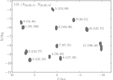
Figure 1 depicts the distribution of the Gaia-ESO bulge
Figure2depicts the selection in color and magnitude with the
combined VVV photometry for all the fields underlaid. The
sample from iDR4 covers a larger area on the sky than previous data releases(see, e.g., Rojas-Arriagada et al.2014), giving us more scope to constrain trends with on-sky position. Each of
our fields contains between 80 and 250 stars. TheGaia-ESO
bulge selection consists of a color cut in each field of
(J-K)0 >0.38, which is then reddened appropriately given
the extinction in that direction, and a magnitude cut
<J <
12.9 0 14.1, which is also modified in some fields to
allow both red clump populations to be represented in the sample(for more details, see Rojas-Arriagada et al.2014).
3. KINEMATICS AS A FUNCTION OF METALLICITY
Based on the clearly bimodal structure of our sample in the
[a M]–[M H]plane, shown in Figure3, we split the sample by metallicity. We dub stars with[M H]>0 as“metal-rich”and stars with[M H]<0 as“metal-poor.”This gives a sample of 1222 metal-poor stars and 716 metal-rich stars. The metal-poor sample is also α-rich, whereas the metal-rich sample is more disk-like(α-poor). We then separately analyze the kinematics of each of these samples across our 12 fields. We correct for solar motion using a local circular speed of 240 km s-1 and solar reflex motion of (11.1, 12.24, 7.25 km s) -1 (Schönrich et al.2010).
The Gaia-ESO sample exhibits features that have been
observed in other studies(for a summary, see Babusiaux2016).
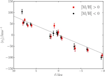
Figure 4 shows the strong correlation between mean line of
sight velocity and Galactic longitude, indicative of rotation. Here, wefind no discernible difference between the rotational signature in the metal-rich stars and the metal-poor stars, both of which show a velocity gradient of ~8 km s-1deg-1. The dispersion and shape of the line of sight velocity distributions of each population, however, show marked differences. Figure 5 depicts the line of sight velocity dispersion of the stars as a function of latitude. The metal-rich stars exhibit a steep decline in velocity dispersion with latitude. A simple linear fit gives a gradient of 7.40.7 km s-1deg-1. The
metal-poor stars, on the other hand, present a much flatter
dispersion profile, with slope 2.01.0 km s-1deg-1. This
property has been seen in other surveys (see Figure 4 of
Babusiaux 2016) and has been shown to be consistent with
specific numerical simulations (e.g., Babusiaux et al. 2010). The evident separation in both chemistry and kinematics is suggestive that the two sequences have different formation histories. We might also expect interesting or unusual features in the line of sight velocity distributions. For example, Nidever et al. (2012) first detected cold, high-velocity peaks in the
APOGEE bulge fields near the Galactic plane, and Molloy
et al.(2015a)subsequently proposed that these structures were a consequence of stars on resonant orbits in the bar(see also Debattista et al.2015for a related idea).
Further examples of this type of phenomenon, now only in the velocity distributions of theGaia-ESO metal-rich sample,
are shown in the two leftmost panels of Figure 6. Fields 5
(Baade’s window)and 6 are of particular interest because they lie along the minor axis of the bar, where the X-shape is observed (e.g., Gonzalez et al. 2015). They are also close Figure 1.Distribution of our sample in Galactic longitude and latitude. Each
field is labeled by its ID number, followed in brackets by the number of stars with[M H]<0and the number with[M H]>0.
Figure 2.Selection of theGaia-ESO bulge targets in color and magnitude. The contours are of the combined VVV photometry from all of thefields, and the purple points represent our sample.
enough to the Galactic plane that the density of the boxy– peanut bulge is still relatively high, so the proportion of metal-rich stars is favorable compared to other minor axis fields at higher latitudes. The velocity distributions for these fields are multimodal, with narrow peaks at non-zero line of sight velocities. Atfield 5(Baade’s Window), there are three narrow peaks; at field 6, there are two broader peaks separated by a small valley. Such features are present in other fields and are particularly prominent atℓ~ 0 , along the short axis of the bar.
4. RESONANT ORBITS IN THE BULGE
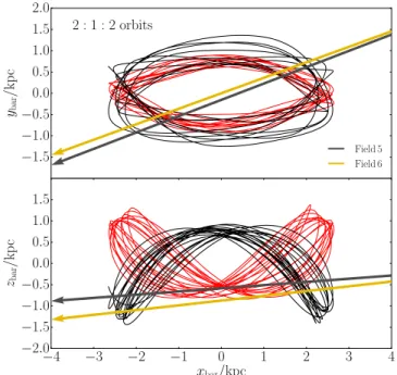
Orbits in the Galaxy are usually characterized in terms of three frequencies, κ, Ω, and ν, describing oscillations in the radial, azimuthal, and vertical directions, respectively. The bar
bar. Resonances also exist in which the vertical frequency
becomes commensurate with κ and W - Wb. “Banana,” or
2:1:2, orbits are examples of this kind of resonance in which there are also two vertical oscillations per revolution, as shown in Figure7.
Here, we will use the sample of resonant orbits extracted by the method of Molloy et al.(2015b)from a simulation of Shen et al. (2010). The bar is formed from m=2 instabilities in a massive disk that subsequently become unstable to buckling
(e.g., Raha et al. 1991). The endpoint of the simulation is a boxy bulge with a pattern speed of∼40 km s−1kpc−1(Shen & Li2016). When viewed at an angle of 15°, the modelfits the mean motion and velocity dispersion data on the minor axis
(b = 0 ), as well as a sequence of longitudinal fields for
= -
b 4 and b= - 6 (see Figure 4 of Shen et al. 2010for
more details). We show as green triangles in Figure 5 the
velocity dispersion of the simulation particles in theGaia-ESO fields as a function of latitude. The simulation matches the behavior of the velocity dispersion of the metal-rich stars. Although we cannot reasonably expect this simulation to be a highly accurate match to the inner Milky Way, its structural properties and gross kinematics are broadly correct.
There is substantial degeneracy in the way in which different orbits can be superposed to make a triaxial bar model. The simulation is a useful tool for understanding which types of orbit are likely populated, but we do not expect the relative proportion of these orbits to be correct for the Milky Way bar. If the data set were much larger, we could perform Schwarzs-child modeling: the relative weights of the orbital families
extracted from the simulation would be fitting parameters.
However, since the data are sparse, it is unrealistic to expect to constrain quantitatively the actual proportions of the different families. Our study is less ambitious: we seek tofind signs in the data that are suggestive of specific orbital families being highly populated. Using the method of Molloy et al.(2015b), we extract the periodic orbits lying on the 2:1, 3:1 and 5:2 in-plane resonances from the simulation by requiring(W - Wp) k
to equal m/n within some tolerance
=0.1. A heliocentric distance cut of 6.8<D kpc<14 has been applied to the simulation data. The distance selection function ofGaia-ESO is much more complicated in reality, but this is a simple and plausible cut to use when comparing the simulations to the data. Finally, we also extract the banana orbits from the 2:1 sample with the additional cut0.9<n k<1.1. The velocityhistograms provided by these orbital families in Gaia-ESO
fields 5 and 6 are shown in Figure6. Field 5(Baade’s window) is relatively well sampled because of the low reddening. The Figure 4.Mean line of sight velocities as a function of longitude. At each
longitude, the red squares (metal-rich) and black circles (metal-poor) are slightly offset from one another for clarity. Both the metal-rich and metal-poor samples exhibit the usual rotational signature seen in bulge stars. The line is a linearfit to the data with gradient8.4 km s-1deg-1. The rich and
metal-poor rotation curves are both consistent with this value at a1slevel.
Figure 5.Line of sight velocity dispersion as a function of latitude. At each latitude, the red squares (metal-rich), black circles(metal-poor), and green triangles(simulation)are slightly offset from one another for clarity. The metal-rich stars in our sample become significantly colder as∣ ∣b increases, whereas the metal-poor stars are consistent with being one temperature. The two lines are simple linearfits to the data. The metal-poor stars have a velocity dispersion gradient of 2.01.0 km s-1deg-1, whereas the metal-rich stars have a
gradient of 7.40.7 km s-1deg-1. The green triangles show the velocity
high-velocity peaks in the data resemble banana orbits moving toward us (predominantly on the near-side,v ~ -90 km s-1) and away from us(far-side,v ~140 km s-1). There is also a
narrow peak in the data at v»0, which is likely a
combination of disk contamination and other resonances
(e.g., 5:2 and 3:1). In field 6, there are possible peaks at
~40 km s-1. Finally, we note a possibly related result—a very narrow velocity minimum on the Bulge minor axis was also reported in red clump stars in Appendix A of Ness et al.(2012).
If the multimodal structure of the velocity histogram of metal-rich stars in Baade’s Window is due to banana orbits, then we would expect to see their signature in other
well-sampled minor axis fields. The second row of Figure 6
shows this is possibly the case. Field 6 is centered on
(ℓ= 0 . 16,b = - 6 . 03). The bimodality of the velocity histogram data is also matched in the velocity distribution of the banana orbits. There is, however, a discrepancy in the location of the velocities of the two peaks. This, however, is controlled by the curvature of the banana orbits and so may be adjusted by changing the potential of the bar. In the other minor axisGaia-ESOfields, the bar density has dropped significantly, and with it the number of metal-rich stars in eachfield. This leads to noisier histograms.
Since we are dealing with relatively few stars, assessment of the significance of the peaks in the data is necessary. Wefitted Gaussian mixture models to the velocity distributions infields 5 and 6 using the SCIKIT-LEARNmodule for PYTHON(Pedregosa
et al.2012). We then approximated the evidence for a given number of Gaussian components using the Bayesian informa-tion criterion(BIC). The BIC offsets changes in the maximum likelihood for a given number of Gaussians by a penalty factor for introducing more parameters. For the metal-poor stars, only one Gaussian component is favored infields 5 and 6, which is consistent with the hypothesis that they belong to a dynamically simpler spheroid. For the metal-rich stars, we found that two components were favored in field 5 (Baade’s window), so that the central peak and leftmost peak in the data are combined into a single Gaussian and the rightmost peak is Figure 6.Line of sight velocity distributions of stars infield 5(Baade’s window)andfield 6. The red(black)filled histograms represent the metal-rich(metal-poor) stars. The velocity histograms of some of the dominant resonant orbits from the simulation of Shen et al.(2010)extracted by the method of Molloy et al.(2015b)are shown in the remaining panels, with the“banana”orbits shown infilled yellow. The same bins are used in each row of histograms. There is a striking resemblance between the velocity peaks in the metal-rich stars and those produced by the 2:1:2 resonance. The metal-poor stars do not appear to possess the same structure.
the second Gaussian. Infield 6, the BIC informs us that only
one Gaussian component is necessary before overfitting the
metal-rich velocity data. According to this particular method, then, the evidence for bimodality in field 6 is actually weaker than our eyes might have us believe. Nonetheless, we believe that taken together the velocity distributions of thesefields are interesting. Furthermore, we would expect some level of disk contamination in both of thesefields at aroundv ~0 km s-1, the removal of which could increase the significance of the bimodality. The expected level of foreground disk
contamina-tion in the two fields using the Besançon model (Robin
et al.2003)is∼5%. Infield 5(Baade’s Window), wefind that 11% of stars have-10<v km s-1<10. Given our estimate
of the contamination, a significant fraction of the stars
contributing to the central peak in the velocity histogram of metal-rich stars are likely disk stars.
Another intriguing feature in the data is that, in Baade’s window, the line of sight velocity and K-band magnitude are correlated(see Figure8). This is predicted by the simulation, so that stars in the high-velocity peak are found on the far
side of the bar (larger K magnitude). The stars with
~
-v 0 km s 1 are generally found at brighter magnitudes, consistent with the picture that they are contaminants from the disk. Interestingly, we do not see the same correlation in field 6.
5. CONCLUSIONS
We compared the velocity histograms of the metal-rich
([M H]>0)stars in theGaia-ESOfields on the minor axis of the Galactic bulge with those produced by the most populated resonant orbits in anN-body simulation of a buckled bar. The narrow peaks that are seen in the data resemble those produced by the “banana” or 2:1:2 resonant orbits in the simulation. Though these results are intriguing, more statistics are required
to confirm the hypothesis that 2:1:2 orbits are heavily
populated in the Galactic bar.
This work supplements the earlier kinematic study of Vásquez et al. (2013). Targeting the bright and faint red
The weighting of the different resonances tells us about the conditions under which the boxy bulge formed via the buckling instability. Metallicity gradients in the original barred disk will cause stars with different radii and hence metallicities to be mapped onto different vertical resonances. This in principle offers us an opportunity to map out the history of buckling in the inner galaxy, as well as trace back the state of the pristine disk in the epoch before buckling.
Based on data products from observations made with ESO Telescopes at the La Silla Paranal Observatory under programme ID 188.B-3002. These data products have been
processed by the Cambridge Astronomy Survey Unit(CASU)
at the Institute of Astronomy, University of Cambridge, and by
the FLAMES/UVES reduction team at INAF/Osservatorio
Astrofisico di Arcetri. These data have been obtained from the
Gaia-ESO Survey Data Archive, prepared and hosted by the
Wide Field Astronomy Unit, Institute for Astronomy, Uni-versity of Edinburgh, which is funded by the UK Science and Technology Facilities Council. This work was partly supported by the European Union FP7 programme through ERC grant number 320360 and by the Leverhulme Trust through grant RPG-2012-541. We acknowledge the support from INAF and Ministero dell’Istruzione, dell’Università e della Ricerca
(MIUR) in the form of the grant “Premiale VLT 2012.”The results presented here benefit from discussions held during the
Gaia-ESO workshops and conferences supported by the
European Science Foundation (ESF) through the GREAT
Research Network Programme.
REFERENCES
Babusiaux, C. 2016, PASA, in press(arXiv:1601.07761) Babusiaux, C., Gómez, A., Hill, V., et al. 2010,A&A,519, A77
Debattista, V. P., Ness, M., Earp, S. W. F., & Cole, D. R. 2015, ApJL, 812, L16
Gilmore, G., Randich, S., Asplund, M., et al. 2012, Msngr,147, 25 Gonzalez, O. A., Zoccali, M., Debattista, V. P., et al. 2015,A&A,583, L5 McWilliam, A., & Zoccali, M. 2010,ApJ,724, 1491
Miralda-Escude, J., & Schwarzschild, M. 1989,ApJ,339, 752
Molloy, M., Smith, M. C., Evans, N. W., & Shen, J. 2015a,ApJ,812, 146 Molloy, M., Smith, M. C., Shen, J., & Evans, N. W. 2015b,ApJ,804, 80 Nataf, D. M., Udalski, A., Gould, A., Fouqué, P., & Stanek, K. Z. 2010,ApJL,
721, L28
Ness, M., Freeman, K., Athanassoula, E., et al. 2012,ApJ,756, 22 Ness, M., Freeman, K., Athanassoula, E., et al. 2013,MNRAS,432, 2092 Ness, M., Zasowski, G., Johnson, J. A., et al. 2016,ApJ,819, 2
Nidever, D. L., Zasowski, G., Majewski, S. R., et al. 2012,ApJL,755, L25 Pedregosa, F., Varoquaux, G., Gramfort, A., et al. 2012, arXiv:1201.0490 Pfenniger, D., & Friedli, D. 1991, A&A,252, 75
Portail, M., Wegg, C., & Gerhard, O. 2015,MNRAS,450, L66
Raha, N., Sellwood, J. A., James, R. A., & Kahn, F. D. 1991,Natur,352, 411 Robin, A., Reylé, C., Derrière, S., & Picaud, S. 2003,A&A,409, 523 Rojas-Arriagada, A., Recio-Blanco, A., Hill, V., et al. 2014,A&A,569, A103
Schönrich, R., Binney, J., & Dehnen, W. 2010,MNRAS,403, 1829 Shen, J., & Li, Z.-Y. 2016, Galactic Bulges,418, 233